HAL Id: hal-03052422
https://hal.archives-ouvertes.fr/hal-03052422
Submitted on 18 Dec 2020
HAL is a multi-disciplinary open access
archive for the deposit and dissemination of
sci-entific research documents, whether they are
pub-lished or not. The documents may come from
teaching and research institutions in France or
abroad, or from public or private research centers.
L’archive ouverte pluridisciplinaire HAL, est
destinée au dépôt et à la diffusion de documents
scientifiques de niveau recherche, publiés ou non,
émanant des établissements d’enseignement et de
recherche français ou étrangers, des laboratoires
publics ou privés.
SPAWN: An Iterative, Potentials-Based, Dynamic
Scheduling and Partitioning Tool
Jean-Charles Papin, Christophe Denoual, Laurent Colombet, Raymond
Namyst
To cite this version:
Jean-Charles Papin, Christophe Denoual, Laurent Colombet, Raymond Namyst. SPAWN: An
Itera-tive, Potentials-Based, Dynamic Scheduling and Partitioning Tool. International Journal of Parallel
Programming, Springer Verlag, 2020, �10.1007/s10766-020-00677-9�. �hal-03052422�
computations of highly variable cost over time can occur. Distributing the un-derlying cells over manycore architectures is a critical load balancing step that should be performed the less frequently possible. Graph partitioning tools are known to be very effective for such problems, but they exhibit scalability prob-lems as the number of cores and the number of cells increase. We introduce a dynamic task scheduling and mesh partitioning approach inspired by physical particle interactions. Our method virtually moves cores over a 2D/3D mesh of tasks and uses a Voronoi domain decomposition to balance workload. Dis-placements of cores are the result of force computations using a carefully cho-sen pair potential. We evaluate our method against graph partitioning tools and existing task schedulers with a representative physical application, and demonstrate the relevance of our approach.
Keywords Simulation · dynamic load-balancing · graph partitioning · tasks ·
SPAWN: An Iterative, Potentials-Based, Dynamic
Scheduling and Partitioning Tool
Jean-Charles PAPIN · Christophe DENOUAL · Laurent COLOMBET · Raymond NAMYST
1 Introduction
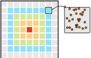
Many physics simulation applications rely on large meshes where each cell contains a few elementary computing elements (e.g. particles, finite elements) and is linked to its neighboring cells. Figure 1 illustrates the concept of mesh and neighboring dependencies. The computing cost of each cell varies with the modeled material and the applied action (e.g., shock wave or distortion). Thus, distributing cells among computing units must both preserve locality of neighbors and dynamically balance computing load. Mesh partitioning can either be achieved by using generic task scheduling or graph partitioning tools. Along with specific libraries [2, 12, 19] and languages extensions [14], many languages now integrate task support in their standard, such as C++11 with its future variables concept. Tasks are generally associated with a data set and can exchange data with other tasks, allowing to define affinity criteria for a
Jean-Charles Papin
CMLA, ENS-Cachan, 61 avenue du Pr´esident Wilson 94235 Cachan, FRANCE,
E-mail: [email protected] Christophe Denoual · Laurent Colombet CEA, DAM, DIF, F-91297 Arpajon, FRANCE Raymond Namyst
Universit´e de Bordeaux, 351 cours de la Lib´eration, 33405 Talence, FRANCE
Fig. 1 2D Mesh example. The red cell has 8 direct neighbors, 16 2ndrank neighbors and 32
3rdrank neighbors. Every cell contains a set of elementary elements (atoms, finite elements or finite difference cells).
given task. Therefore, a particular attention shall be paid to the place (i.e., the computing unit) where the task will be executed. The still increasing cores-on-chip number [7] forces applications to spawn a large number of tasks so as to prevent cores from entering a starving state. This eventually leads to an important complexity as task scheduling is known to be an NP-Complete [20] problem. Moreover, existing dynamic task scheduling policies minimize the overall computing time and/or data displacements. By doing so, they do not necessary ensure the compactness of the set of cells to be exchanged, thus possibly increasing the cost of communications when physical models involve many neighbor-to-neighbor communications.
On another hand, graph partitioning tools can be used to build compact sets of mesh. Several well known libraries exist [15, 11, 6] and provide high-quality partitioning algorithms. The NP-Complete problem is handled by using multi-levels algorithms [8] that successively reduce a graph into a smaller graph that can be partitioned with standard heuristics: the result is then successively propagated into the original graph. Such algorithms require to merge some nodes into bigger nodes, and thus, require to select graph nodes. This property is known to be limiting: in a distributed environment, such algorithms need to communicate a lot. With upcoming architectures (i.e., manycore) and with the still increasing computing clusters size, we definitely need algorithms that involve a limited amount of communications.
We present Spawn, a physical interaction inspired scheduler that produces compact and optimal Voronoi domains. In our case, Voronoi diagrams max-imize per-core data locality by providing numerous advantages: cache usage improvements, more efficient NUMA-aware memory allocations/accesses and less Point-to-Point communications. This scheduler has the advantage of being ef-ficient to compute and offers an automatic refinement. This scheduler can be used as a task scheduling algorithm as well as a mesh partitioning tool. This paper is organized as follows: section 3 presents the rationale behind using physical interactions for dynamic scheduling while section 4 focuses on imple-mentation details and some preliminary evaluations. Following sections present a set of experiments that compare our approach with graph partitioning tools (section 6) and dynamic task schedulers (section 7). Concluding remarks and future work are discussed in the last section.
2 Context
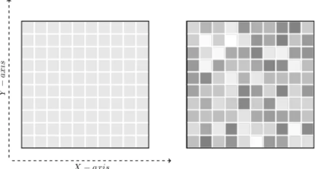
Applications of physics modeling mainly encounter two load variation scenar-ios: randomly diffused load or a continuous load variation, both over time. We build a grid of tasks that corresponds to the modeled material with an analogy between sets of elements (atoms, finites elements) and computing tasks. In this case a task is essentially a dataset on which we regularly apply some comput-ing functions. Figure 2 represents the set of cells on a multi-dimensional grid. Each cell has its computing cost of its own that can evolve over time.
t = 0 t = 1 t = 2 Random Sho ck-W a v e
Fig. 2 Grid of tasks with an evolving task cost. Each square represents a task, and the brightness represents the cost of the task: dark cells are more costly than white ones. Each task contains a set of the physics elements of the simu-lated domain.
Distributing all these cells among computing units is complex and several tools or methods exist. As a consequence of neighboring dependencies (see fig. 1), we must distribute cells into compact sets. These sets must be as con-servative as possible among successive scheduling steps in order to prevent data displacements. A common way to achieve this is to move sets bound-aries (see fig. 3). However, such decomposition induces an unstable number
t = 0 t = 1
Fig. 3 Regular domain decompo-sition at t = 0 (left) and t = 1 (right). When moving upper and/or lower boundaries, the number of connected neighbors can strongly vary.
of neighbors over successive scheduling: moving upper and lower boundaries modify the number of connected neighbors too.
Graph partitioning tools [15, 11] can also be used to distribute tasks. By exploiting the fact that tasks have strong affinities with their neighborhood (see fig. 1), such meshes can directly be represented by graphs where each node is a task, and where a link is a neighboring connection. Partitioning tools provide very efficient algorithms for very large regular and non-regular graphs, which can take into account affinity characteristics. Nevertheless, such tools do not perform well when dynamic scheduling is required. If graph
re-finement (i.e. the ability to update current partitions) is not supported, slight
task weight variations usually lead to the generation of a completely different graph partition, which incurs numerous data transfers to re-assign tasks. Par-allel algorithms involved into distributed versions of partitioning libraries [5, 10, 6], while offering refinement functionalities, suffer of scalability issues as we will see in section 6. In modern architectures (i.e. the Intel R Xeon Phi),
the number of cores is significant (typically 61 cores for Intel R Xeon Phi 7100
series) and the number of available thread units doubles or quadruples this value. The amount of memory per core is consequently a limiting factor (less than 300 Megabytes that must be shared among threads) and low memory footprint load balancing mechanisms must be designed.
3 Load Balancing with Molecular Dynamics
One major contribution of this article is the integration of concepts coming from Particle Dynamics (PD) simulations, a type of N-Body simulations, into workflow scheduling. This section first describes how we use particles as Voronoi seed to tessellate the volume, and how an analogy with particles with electrostatics interactions is used to optimize the scheduling method. We will then explore how we target the optimal per-core load with this method and finally the way we translate the computing load into forces.
3.1 Using Particles to Assign Work to Processing Units
3.1.1 Set of Objects to Schedule
We define the elements to be scheduled between computing units as a grid of objects. Objects can be of different nature (atoms, finite element, computing task or graph node). The only two important properties of the grid are its dimensions (x, y, z, with x, y, z ∈ N) and its definition in the Euclidean space, allowing distance computations. Each cell of the grid has thus a specific coor-dinate (x, y, z, with x, y, z ∈ N) on the grid and a specific computing cost (see figure 4). Because of the geometric properties of the grid, neighboring cells of the grids can be seen as interconnected cells: a neighboring relation can be assimilated to a connection between two distinct tasks or graph nodes.
X− axis
Y
−
axis
Fig. 4 The task grid model: the grid has a dimension (x, y, z, with x, y, z ∈ N) and is defined in the Euclidean space. Each cell has a specific coordinate and computing cost (right figure: darker cells have a more important computing cost than white cells).
We define a vCore as a virtual representation of a computing unit. When seen from the PD side, a vCore i is a particle: it has coordinates (in the Euclidean space, with x, y, z ∈ R), a velocity vector and force vector. A vCore can be positioned inside the previously-defined grid. When seen as a computing unit, a vCore ‘i’ has a computing load Qi defined as the sum of computing loads of its set of tasks. A relationship between electrostatics charges and the
computing load is proposed in paragraph Particle dynamics (page 7) to complete the proposed analogy.
3.1.2 Tessellation
The assignment of cells to vCores (and thus, to computing units) resides in the partitioning of the previously defined grid. This work uses a Vorono¨ı [13] tessel-lation to assign cells to the underlying computing units. A Vorono¨ı tesseltessel-lation is a geometric partitioning based on distances between points. Vorono¨ı dia-grams gather a set of points around a central point: the site of a Vorono¨ı cell (see figure 5). In our case, sites of Vorono¨ı cells are defined by the location of our computing units (or vCore), and cells of the domain are our set of tasks (or node graph) to compute. Thus, distributing tasks to computing units is as easy as computing distances between set of points. The complexity of com-puting distances between points is linear in n (n · O(m), with n, the number of sites, and m, the number of cells), but specific methods can dramatically reduce this complexity to O(log(n)). Since the computing load Qi of a vCore
Fig. 5 Vorono¨ı tessellation. On the left figure, Vorono¨ı sites are positioned on the cell domain. The right figure shows the cell distribution into Vorono¨ı cells, characterizing the task distribution over underlying computing units.
i is the sum of tasks load inside its vorono¨ı zones, obtaining load equilibrium
between vCore therefore consists in finding the vCores locations (and thus the Voron¨ı tessellation) that ensures equality between all Qi.
We chose to use Vorono¨ı diagrams since they offer compact and convex sets and have geometric stability [16]. They are used in many scientific ap-plications (e.g., in physics [4], geography [17] and biology [3]). Interestingly, the compactness of the Vorono¨ı sites arrangement plays an important role regarding the partitioned shapes, both in terms of surface of Vorono¨ı zones and sites connectivity. For example, the Vorno¨ı tessellation of a compact set of points in 2D leads to hexagonal shaped zones, and thus to the minimal perime-ter/surface ratio compared to a simple square grid. In 3D, a compact set of points (e.g., points ordered following a face centered cubic lattice) tessellates the volume into regular rhombic dodecahedra, a space-filling polyhedra that also maximizes the surface to volume ratio.
Applied to our analogy between vCores and particles, a compact set of vCores minimizes the amount of surface, and therefore the number of cells
located on the boundary of the vCore domain. Compared to a cubic arrange-ment of Vorono¨ı sites, the number of neighbors of a vCore (i.e., the number of neighboring sites sharing a surface, a line or a point with a vCore) is reduced from 26 to 12, an interesting advantage when one want to limit the number of site-to-site communications.
The interaction between particles, presented in the following section, is designed to favor the compactness of the Vorono¨ı sites arrangement as well as to allow for a handy control of the Qi optimizing procedure.
3.1.3 Particle Dynamics
A computing unit is associated to a Vorono¨ı site (a particle) and to the corre-sponding tasks of the cells contained in its Vorono¨ı zone. Particles arrangement thus define the way the objects to be scheduled are assigned. To design the interaction between particles, we have decided that the interactions should favor compactness of the site arrangement to minimize the number of site’s connections, and that the calculation of the new partition should be done fre-quently so that its computational cost to achieve equilibrium must be marginal compared to the overall computations.
We consider in the following example of electrostatics interaction, a very interesting pair force candidate based on the Coulomb’s interaction and pro-ducing compact structures (for homogeneous charges) at a very low computa-tional cost. For two particles i and j, separated by a vector rij = xi− xj, the electrostatic force is:
Fij = λij
rij |rij|3
, (1)
with λij a function of the loads (Qi and Qj) of the interacting vCores to be defined in next section (note that λij is the product of particle’s charge in a standard Coulomb’s interaction).
Focusing on the equilibrium only, we use a damped relaxation of the forces by expressing velocities as a factor of applied forces:
vi = dxi
dt = −αFij (2)
with α, a positive scalar. We also lump α with pseudo-time increment into a simple scalar k:
xi(t + ∆t) = xi(t) − k X
j
Fij (3)
We rescale k for every step so that the distance x(t) − x(t − ∆t) is a fraction of the cell box dimension, which ensures a rapid convergence to stable states.
3.2 Converging Toward Optimal Load Balance
As explained in previous section, we want to make vCores move so that they reach a position at which, once the tessellation step achieved, equilibrates the load between vCores. Besides the fact that this requires a specific force equation definition, one can note that the exact solution of this problem relies on a global knowledge: we compute forces between pairs of vCores, and we target an optimal load distribution that satisfies the load of all vCores. We define the optimal vCore load m as the sum of the load of all vCores, which is by definition the cost of the whole cell grid, and we divide it by N , the number of vCores. Therefore, m is the average computing load of the whole computing domain: m = 1 N N X i=0 Qi (4)
Since this optimal per-vCore definition would result in a poorly scalable cen-tralized implementation due to need of knowing the load of the cells of the whole domain, we define an approximate per-vcore local optimal that only uses the load of surrounding cells:
mapprox = 1 Ns Ns X i=0 Qi (5)
While this definition is close to the previous one (see equation 4), the resulting solution is no longer exact, and the convergence is toward a local optimal.
Now that our targeted convergence state is defined, we need to define the force equation that takes into account our optimal load distribution.
3.2.1 Force Equation
Forces between particles are proportional to the interaction amplitude λij (see equation 1)), designed in this section so that the vCore load Qi tend to the average load m, targeted by all vCores. The difference m − Qi represents the distance between the load of a particle i and the average (optimal) load m. For two interacting VCores i and j, we take a force proportional to the sum of two distances (m − Qi and m − Qj) instead of the product of charges CiCj in Coulomb’s force definition:
Fij = λ
rij |rij|3
, with λ = 1 − Qi+ Qj
2m . (6)
This force definition, referred to as the MediumLoad potential, produces three kinds of forces: positive, negative and null forces. For two vCores i and j, when the Qi+ Qj sum is smaller than the 2m term, the whole fraction
Qi+Qj
2m is
smaller than 1, and the whole λ is positive, leading to positive forces. Similarly, when the Qi+ Qj sum is larger than the 2m term, the whole fraction is larger
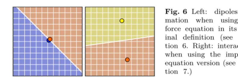
Fig. 6 Left: dipoles
for-mation when using our
force equation in its orig-inal definition (see equa-tion 6. Right: interacequa-tions when using the improved equation version (see equa-tion 7.)
than 1, thus, the λ term is negative leading to negative forces. Lastly, when the Qi+ Qj sum is equal to the 2m term, the λ is null, and forces are null. An equilibrium is thus achieved when all the loads Qi are equal to the target load m.
With two particles, the Qi+ Qj sum is smaller than the 2m term only when the two vCores are under-loaded, and is larger than the 2m term only when the two vCores are over-loaded. When an under-loaded vCore repulses neighboring vCores through repulsive forces, its own Vorono¨ı domain grows by collecting cells. In the same way, when an over-loaded vCore attracts its neighbors through attractive forces, other vCores grab cells from it.
3.2.2 Fixing Dipole Formation
The proposed force equation allows two particles to collapse into a dipole as long as their load are equal to the average load (see figure 6). This brings two major issues: vCores spinning and, when the distance tends towards zero, to a singularity (division by zero). To eliminate this degenerate state, we have then added a repulsive term, also known as a short repulsive term, ensures a minimal distance between two vCores:
Fij= λ rij |rij|3 + ν rij |rij|5 , with λ = 1 −Qi+ Qj 2m . (7)
with ν a parameter tuned to have a minimal distance between particles about the size of cell box dimension.
4 Implementation Details & Preliminary Evolution
4.1 Global Vs Local Targeted Load
As previously described, we have defined two ways to regulate the load be-tween computing units. A global one, that requires the global knowledge of costs of all tasks of the domain and that requires to compute forces between all pair of vCores. The second one considers only local interactions, and lo-cal information. Thus, it relies on a neighbor list, and does the whole load balancing step by using only this local information (reduced set of cells, re-duced set of vCores). Figure 7 presents these two force schemes. While this second option has good parallel opportunities (i.e., only local node-to-nodes
Fig. 7 Two interaction schemes. Left: fully centralized one based on global knowledge. In this scheme, every vCore needs to know the cost of all cells, and to communicates with all others vCores. Right: local interactions only. Here we consider only neighboring nodes and cells.
communications), this scheme implies two drawbacks: we consider only the local particle system instead of N-Body system, leading to a non-perfect so-lution to initial load balancing problem. Therefore, the second disadvantage is that we could have a higher number of iterations of the particle dynamics main loop algorithm to reach the targeted optimal load.
4.2 Tasks Assignment: Centralized Vs Distributed
Task assignment is also a critical point because it depends on the position of vCores, i.e., we partition the cell domain by using the final position of vCores. We use two distinct algorithms to perform cell assignment: a fully sequential one and a fully distributed one based on the only-node-to-node communication model. The first one (see algorithm 1) is to be computed by a single core, and thus, in a distributed memory environment it requires a lot of All-To-One communications. The second one, presented in details in section 4.4,
Algorithm 1 Vorono¨ı Tessellation searchTree ← buildTree (setOfvCores) for c in cells do
closest ← searchTree.findClosest (c) setOfvCores [closest].assignCell (c) end for
is able to compute the Vorono¨ı tessellation in parallel (i.e., each computing unit computes its own Vorono¨ı tessellation) by using only communications to neighboring nodes. To do so, this algorithm needs to know the position of the local vCore inside the domain and the position of its neighbors. With these two information, a vCore can then evaluate whether a cell is inside its local Vorono¨ı zone or not. We recall that this step consists in closest-element search. We don’t want each vCore to iterate over all cells of the domain, and by using
the bounding box of the Vorono¨ı zone n, we reduce the set of cells on which we iterate to deduce the Vorono¨ı zone n+1.
4.3 Parallel Force Computation
Because of the weak impact of long-range interactions, we can avoid to com-pute forces between all pair of particles. Therefore, in parallel, we consider only first and second-rank neighboring interactions: every node knows the comput-ing load of its neighborcomput-ing nodes and can thus deduce all locally-applied forces by its neighbors. However, because of the of our potential definitions (see sec-tion 4.1), this parallel force computasec-tion step is limited by the way we deduce the optimal per-core load (i.e., fully centralized or with local interactions only).
4.4 Different Versions
In order to clearly evaluate our method, we have designed several versions of our load balancing model.
Version 1 (V1): sequential algorithms, exact solution In this version, we use
only a single computing unit to compute the force iterations and the cell distributions between all other computing units. As presented in algorithm 2, we have to perform global All-To-One communication steps (blocking step).
Algorithm 2 Vorono¨ı Tessellation ...
receiveCellCostInformationFromALL () mainConvergenceLoop () // load balancing step for v in setOfvCores do
sendCellAssignment () end for
...
Version 2 (V2): distributed algorithms, exact solution In this version, we use a
distributed cell assignment and force computation, but with the global optimal load. The main convergence loop is presented in algorithm 3: In this version, the computeLocalF orce() step relies on a All-To-All communication in order to retrieve the global optimal m value presented in equation 6
Version 3 (V3): distributed algorithms, local solution This version is exactly
the same as the V2 but the computeLocalF orce() step no longer relies on a global communication scheme. Instead, we deduce the local optimal m of equation 6 by using the load information of our neighbors.
Algorithm 3 PSpawn Main Convergence Loop. We first need to synchronize
(line 2) neighbor information (due to the newest local computing load). Local force and thus, new local position can be computed (lines 3 and 4). We then need to synchronize (line 5) position information before computing the local Vorono¨ı domain (line 6). The last step (line 7) exchanges costs of tasks that leave/arrive into the local domain.
1: for all Convergence Step do
2: synchronizeNeighbors () 3: computeLocalForce () 4: ComputeNewLocalPosition () 5: synchronizeNeighbors () 6: computeLocalVorono¨ı () 7: exchangeCosts () 8: end for 5 Benchmark Application
This section presents results of our scheduling library (Spawn). In order to evaluate our scheduler, we have developed a representative stencil-like model applications (see table 1). This benchmark application uses a real cell domain (with evolutive load, see figure 8) and provides an intensive memory usage with data exchanges between cells. Every cell has 4 direct neighbors (four car-dinal directions), and requires data (a matrix of double) from its neighbors to compute its own matrix. These exchanged matrices are the result of the previous iteration. In a distributed memory (see section 6.1.1), this allows us to evaluate the number of MPI communications induced after the new domain decomposition and during computation (data exchange between meshes). We evaluate our scheduler with sequential partitioning tools and parallel partition-ing tools (with partitionpartition-ing refinement enabled). In section 7, we evaluate the same application, but in a shared memory, by comparing our scheduler against common task scheduling strategies. Our analysis focuses on cache miss rates.
Table 1 List of benchmark applications and their properties
App No Parallelism Matrix size Memory Focus
#a pThreads 8x8 Shared Cache misses
t = 0 t = 1 t = 2 t = 3 t = 4
Fig. 8 Generated load evolution: each square represents a task, and the color represents the cost of the task: dark cells are more costly than the white ones, i.e, we do more computations on internal matrices.
6 Comparison with Graph Partitioning Tools
6.1 Shared Memory: Application #a
In a shared memory environment, memory accesses must be handled with care to avoid performance bottleneck. Due to hierarchical memory organisation (several NUMA nodes, several cache levels), the data locality, usage and re-usage are mandatory to get good performance. In this section, we compare performance and data cache misses ratio and show how the Spawn library improves this ratio in both static and dynamic load evolution (see figure 8).
6.1.1 Spawn-V1 VS Graph Partitioning Tools
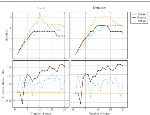
Figure 9 compares performance of Spawn (version V1) in relation to Scotch [15] and Metis [11] libraries. Scotch supports graph refinement and all experiments featuring Scotch exploit this functionality. Left figures refer to the static load case while right charts refer to the dynamic load evolution case, and, upper charts refer to the speedup while the bottom ones refer to the average number of L1 data cache misses per thread for one iteration.
All partitioning strategies produce compact sets, minimizing data transfers between tasks, but Spawn has better performance in both static and dynamic load variations. Graph partitioning tools may not support graph refinement (e.g. Metis) and thus, produce a new and totally different task distribution after a task cost variation. Due to hardware and Operating System behavior, a task cost may vary over time, even if it’s the same task and it does the same type of computation. Hence, such partitioning tools produce different task distributions after each iteration. This involves data displacements between sockets and higher cache miss rates (see bottom charts in figure 9).
6.2 Distributed Memory: Application #2b
Distributed memory implies to send data over a transfer bus (a network, a Pci-E bus, and so forth). Therefore, high contentions can occur upon a large data transfer, and especially when several computing nodes exchange data at the same time. In this section, we evaluate Spawn V1 performance against
2 4 6 8 Sp eedup Static Dynamic Spawn Scotch Metis 0 5 10 15 20 0.98 1 1.02 1.04 1.06 Number of cores L1 Cac he Misses Ratio 0 5 10 15 20 Number of cores
Fig. 9 Resulting speedups (top) and L1data cache misses (bottom) with graph partitioning
tools (Scotch, Metis) and with Spawn on an Intel R IvyBridge Xeon E5-2680 computing node.
Scotch is used with refinement strategies (SCOTCH graphRepart routine). Task scheduling or graph partitioning is achieved after each computing iteration. The Spawn cache miss ratio is used as a reference on bottom charts.
sequential and distributed graph partitioning tools. We particularly focus on speedup and on the number of exchanged cells.
6.2.1 Sequential Partitioning Tools
Figures 10 and 11 present the same evaluation but in a distributed memory environment by using MPI libraries. Measurements focus on speedup and data transfer rates between each iteration. We use matrices of 128x128 doubles in a domain of 512x512 tasks. Tests run on a cluster of Intel R Xeon X7650
nodes, interconnected with an Infiniband QDR network. Figure 10 shows the average number of exchanged tasks on the MPI network (in percentage of the entire domain) and the resulting application speedup. Metis involves an important data exchange since it is not designed for dynamic partitioning: nearly the entire task domain is exchanged for each iteration while less than 5% of the domain is exchanged with Scotch and Spawn.
6.2.2 Distributed Partitioning Tools
Tools like PTScotch [5] and ParMETIS [9] can perform parallel graph parti-tioning. ParMETIS supports refinement graph partitioning, i.e., it takes into
0 200 400 600 800 1,000 1
10 100
Number of MPI processes
Exc hanged tasks (%) 0 200 400 600 800 1,000 0 10 20 30
Number of MPI processes
Sp
eedup
Spawn Scotch Metis
Fig. 10 Resulting data transfer rates (left) and speedups (right) with graph partitioning tools (Scotch, Metis) and with Spawn. Scotch is used with refinement capabilities. Scheduling or partitioning is achieved after each iteration.
account the actual partition to produce a new partition with the newest task costs. Scotch does not. Zoltan [6] is another partitioning tool that can use not only its internal algorithms but also Scotch/PTScotch or ParMETIS to compute a graph partitioning. One limitation of these tools is that they need the identifier of each node that owns every local tasks and every neighboring local or remote tasks. This implies to maintain on each MPI node, and after every calls to a partitioning routine, the list of neighboring nodes, and the list of tasks they share.
The next evaluation focuses on Zoltan and ParMETIS (with Zoltan) tools. We evaluate Zoltan with PHG and RCB partitioning algorithms. PHG is the in-ternal Parallel Hypergraph and Graph partitioning method. It supports initial partitioning, refinement and re-partitioning operations. Both repartitioning and refinement operations reuse the current partition, but refinement opera-tion is stricter. With the RCB method we use one internal algorithm opopera-tion, RCB REUSE, that indicates whether previous cuts should be used as initial guess for the current RCB partition. Figure 11 shows data transfer rates and speedups of Zoltan (with PHG, RCB and ParMETIS) in comparison with Spawn. We can see that Spawn performance is similar to graph partitioning and geometric al-gorithms when the network is not used (i.e. one computing node used). For a few number of MPI nodes, Spawn is still better than Zoltan or ParMETIS, while, for a higher number of MPI nodes, RCB algorithm outperforms other algorithms. More precisely, if we compare the RCB algorithm to Spawn, we can see (left chart), that Spawn produces less data transfers (1-3% of the entire domain versus 5-35% for RCB). This explains that our algorithm involves a better speedup when the network is not used (time spent on internal com-munication is regained by the time not spent on exchanging data). On the other hand, with a higher number of nodes, the centralized behavior of Spawn, i.e., the knowledge of the average load and its single-thread implementation,
100 101 102 103 0
10 20 30
Number of MPI processes
Exc hanged tasks (%) 0 200 400 600 800 1,000 0 20 40 60
Number of MPI processes
Sp
eedup
Spawn Zoltan-RCB Zoltan-PHG Zoltan-ParMetis
Fig. 11 Resulting data transfer rates (left) and speedups (right) with Zoltan (RCB, PHG), ParMetis (through Zoltan) and with Spawn. One can notice scalability issues of graph par-titioning tools (PHG and ParMETIS).
is penalizing and collective MPI operations considerably slow down the global computation.
This observation is however incomplete if we compare Spawn to the PHG method or to ParMETIS. In comparison with Spawn, data transfer rates are more important for PHG, and really similar to ParMETIS. Thus, we could expect better results for, at least, ParMETIS. Considering that partitioning tools have scalability limitations because of internal synchronizations, exacerbated by the network, we can consider that data transfers are less penalizing than scalability limitations, which explains PHG and ParMETIS results in figure 11.
6.3 Evaluation of the Distributed Algorithm
This section presents and analyzes induced performance in terms of speedup and number of communications of the Spawn library by using version 2 (V2) and 3 (V3). Experiments are achieved on a cluster of 32 Intel R
Xeon Xeon E5-2698v3 nodes (Haswell architecture, 2x16 cores, 128 Gio of RAM, for a total of 1,024 cores), interconnected with an Infiniband QDR network. We use the same application set as presented in table 1.
We compare performance of the Spawn library in relation with other par-allel graph partitioning tools. As in previous section we compare performance against the Zoltan library. Two internal and one external algorithms are used: RCB (the geometric graph partitioning algorithm), PHG (the graph partitioning algorithm), and the external ParMetis library. A test configuration consists in a grid of 512x512 cells. Each cell contains a matrix of 128x128 double values (128Kio per matrix). Figures 12 and 13 show the cost of our iterative model. The first one presents speedup of our benchmark application over an increasing number of MPI nodes and with an increasing number of PSpawn convergence iterations (I parameter). The second one presents the time spent in main parts of our distributed algorithm. We can first see that the application speedup,
0 20 40 60 80 100 120 I = 1 Sp eedup I = 10
PSpawn (MediumLoad) PSpawn (DistMediumLoad) Zoltan - RCB Zoltan - ParMetis
100 101 102 103 0 20 40 60 80 100 120 I = 20
Number of MPI processes
Sp
eedup
100 101 102 103
I = 40
Number of MPI processes
Fig. 12 Cost of the PSpawn iterative model, successively increasing the number of iterations used to compute a partition. Top left: 1 iteration. Top right: 10 iterations. Bottom left: 20 iterations. Bottom right. 40 iterations.
while greatly enhanced with our PSpawn algorithm, strongly depends on the number of iterations: we lose nearly 35% speedup points with 40 iterations regarding the one with one single iteration. We can also notice that we have a brutal performance drop when using 512 (and more) MPI nodes. One can expect better performance when increasing the number of iterations of the model (I parameter) but results show that best results are achieved with I =
1. This is due to the way our benchmark application is designed: it has a few
computing ratio regarding its communication volume (each cell requires data from its 4 direct neighbors) and it computes a new cells distribution between each of its computing iteration. Therefore, the scheduling step is limiting. In order to confirm this point, figure 14 presents a speedup over 1,024 MPI nodes with the same domain size (512x512 cells) but with a more important amount of computation (x5 factor). We can clearly see that the scheduling step is less penalizing than before.
80 90 100 10 iteration MediumLoad % of Time 90 95 100 20 iteration 90 95 100 40 iteration Voronoi Tessellation Neighboring Com. Local Force Computation
128 256 512 1024 85 90 95 100 10 iteration DistMediumLoad % of Time 128 256 512 1024 90 95 100 20 iteration 128 256 512 1024 92 94 96 98 100 40 iteration
Fig. 13 Cost repartition in our distributed algorithm by using our two distinct version for different number of MPI processes: the V1 (top) and the V2 (bottom). Neighboring communications consist in exchanging local node information (load, position) and in the cell cost exchange between each local Vorono¨ı tessellation: we need to send (or receive) cost of cells that leave (or arrive in) the local domain.
100 101 102 103 0 50 100 150 I = 20
Number of MPI processes
Sp
eedup
Initial Computing x5
Fig. 14 PSpawn performance with a more CPU-bound application (x5 regarding other tests). In this case, scheduling is less penalizing.
Figure 13 shows that most part of the computing cost (more than 80%) of our algorithm remains in the Vorono¨ı tessellation, and since we need to compute a Vorono¨ı tessellation for every single iteration, this explains why the speedup is penalized when we increase the number of iterations. We also see that, as we increase the number of MPI nodes, the part of communications is more important (for both force neighbor communications and force computa-tions). On Figure 15, which shows real time values, we see (left chart) that the Vorono¨ı tessellation cost dramatically decreases with the increase of the number of MPI nodes. The time spent in neighbor-to-neighbor communica-tion (middle chart) slightly increases for a small number of processes (between 1 and 16) but remains however constant for a higher number of MPI nodes.
101 102 103
0 0.5 1
·106
Number of MPI processes
Time (µs ) Voronoi 101 102 103 0 2,000 4,000 6,000
Number of MPI processes Communications 101 102 103 200 400 600 800 1,000
Number of MPI processes Force Computations
Fig. 15 Cost evolution of the Vorono¨ı tessellation, the communication ratio and the force computation steps of the distributed algorithm. Note the 105 scale factor for the cost of
the Vorono¨ı Tessellation chart (right). The vertical red line shows the limit after which the network is involved. Dashed lines represent the cost evolution when using the V2 algorithm.
This is a consequence of our peer-to-peer model: when using a higher num-ber of nodes, communications are limited by the nearly constant numnum-ber of neighbors.
We can also compare the impact of the centralized property of the V1 potential: it requires, during the force computation step, to know the whole task cost of the cell domain, leading to an All-to-all MPI communication. Even if figures 13 and 15 show that we clearly reduce the communication cost during the force computation with the V2 potential, figure 12 shows that removing the global communication required by the V1 potential does not have a significant impact on overall performance. Deeper experiments have shown that the V2 potential is unstable (non-constant quality) and induces several cell movements between each application computing iteration (see figure 16).
Finally, figure 16 presents the average number of exchanged tasks after the computation of new partition. As one can notice, this number slightly increases within the number of iterations. This is an expected behavior since vCores dis-placement is related to the number of iterations. This number is however really similar to the one induced by using graph and geometric partitioning tools. We can also notice the instability of the V2 potential: since vCores do not target a global computing load, they have independent local displacements, leading to oscillations during displacements. In the end, these oscillations induce a lot of non-desirable cells, and therefore data displacements between computing nodes.
7 Comparison with Affinity-Based Scheduling Policies
We have extended the StarPU [2] runtime with our scheduler to evaluate the quality of the Spawn (V1) performance against common task scheduling policies. Data block of tasks are managed by StarPU through the specific starpu block data register routine, which enables automatic and back-grounded data transfers. We evaluate our scheduler on a two-socket Intel R
0 10 20 30 I = 1 Exc hanged tasks (%) I = 10
PSpawn (MediumLoad) PSpawn (DistMediumLoad) Zoltan - RCB Zoltan - Parmetis
100 101 102 103 0 10 20 30 I = 20
Number of MPI processes
Exc hanged tasks (%) 100 101 102 103 I = 40
Number of MPI processes
Fig. 16 Comparison of average induced communication per MPI node after the compu-tation of a new cell distribution with a variable number of iteration steps (I parameter). Top left: 1 iteration. Top right: 10 iterations. Bottom left: 20 iterations. Bottom right. 40 iterations.
runs with a domain of 100x100 tasks, where each task contains a matrix of 8x8 doubles. We evaluate performance in both static and dynamic load variations over time.
7.1 Integration
StarPU comes with a variety of scheduling policies, but also offers the capa-bility to define new ones. This permits to manage StarPU workers (abstract representation of computing units) directly. Spawn is used by StarPU through an intermediate meta-scheduler that implements interfaces required by StarPU (the starpu sched policy C-structure). When tasks are submitted to StarPU, they are forwarded to the scheduling layer, and thus, to our meta-scheduler. This meta-scheduler asks our library to which worker this task should be as-signed (more precisely, to which Vorono¨ı domain this task is attached).
Regular grids or random positions are used to initialize the vCore set, and therefore the first task distribution. Once tasks are distributed among StarPU workers, their execution (e.g. the computing time) is monitored and then sent to our library. The scheduling is computed with nearly no additional cost (see figure 17): it is computed by the first inactive StarPU worker, and as long as
Time
Fig. 17 Timeline representing StarPU calls (grey), task computation (green) and parti-tioning computation with Spawn (red). The scheduling time is fully hidden by computing imbalance.
another worker is still working. Thus, we only compute a task distribution when an imbalance exists. This has also the advantage of allowing us to set
P = 1 and I = 1 as parameters of our algorithm (which can be interpreted
as ”as long as an imbalance exists, do one iteration to reach the most optimal
distribution” ). As explained, a new task distribution is based on the task
information (i.e. computing cost) of the previous task execution. Therefore, the first two load balancing steps are not optimal.
7.2 Results
Figure 18 compares performance of Spawn (V1) in relation to predefined StarPU schedulers. Left charts refer to the static load case while right charts refer to the dynamic load case. Upper charts refer to the speedup while the bottom ones refer to the ratio of L1 data cache misses per thread (per
iter-ation) in comparison with Spawn. We use three internal StarPU schedulers: Eager, DM and DMDA since other schedulers are only useful with heterogeneous machines. Eager uses a simple FIFO-based greedy policy to schedule tasks. DM and DMDA use performance models allowing them to perform smart task place-ment, with the objective to minimize the overall execution time. DMDA works like DM, but takes into account data transfer time during task placement. More information about DMDA can be found in the StarPU HandBook [18].
In both static and dynamic load variation cases, Spawn is close to StarPU schedulers performance and outperforms them with the growth of the number of threads. Bottom parts of figures show that Spawn dramatically reduces the number of L1cache misses with a factor between two and four. This is due to
the Spawn ability to provide geometrically compact sets of tasks, reducing data transfers between threads. On the other side, if we compare cache misses with Eager, DM and DMDA, we note that Eager doubles the number of cache misses that DM and DMDA induce, but has better performance. This is related to the behavior of these schedulers: by using a task queue, Eager naturally maximizes StarPU workers activity, in opposition to DM and DMDA that distribute tasks
in advance as soon as they are ready in order to minimize overall execution
time. Since our application uses intensive memory accesses, the execution time is strongly related to memory accesses, and task execution time depends on the location where tasks are executed. Therefore, assigned tasks by DM or DMDA
2 4 6 8 Sp eedup Static Dynamic Spawn Eager DM DMDA 0 5 10 15 20 1 2 3 4 5 Number of cores L1 Cac he Misses Ratio 0 5 10 15 20 Number of cores
Fig. 18 Resulting speedups (top) and L1data cache misses (bottom) with internal StarPU
schedulers (Eager, DM, DMDA) and with Spawn on an IvyBridge Xeon E5-2680 computing node. The performance drop for nearly 10 core indicates the NUMA-effect. With Spawn, this effect is delayed regarding other scheduling strategies. The Spawn cache miss ratio is used as base on bottom charts.
constitute a set of non-related tasks, like they would have been assigned with Eager. Hence, with DM or DMDA, StarPU workers are imbalanced, since the execution time of assigned tasks does not reflect their real execution time. A deeper analysis of StarPU execution trace (FxT[1] traces, see fig 19) confirms this point. With this information, it appears that common task schedulers are unable to perform efficiently with such task configurations (neighboring and data dependencies).
8 Conclusions
We introduce a new approach to dynamically schedule tasks within domain-decomposition based applications, that borrows many ideas from molecular dynamics simulations. We combine physical particle interactions and Voronoi domain decomposition to virtually move cores over a 2D/3D mesh to partition the set of application tasks. We have designed three versions with either cen-tralized or distributed properties. In a shared memory environment, or with a few number of MPI nodes (around 256), experiments show that the fully cen-tralized version outperforms well known graph partitioning tools and common task schedulers. Versions with distributed algorithms improve scalability while
Fig. 19 FxT traces with the DM scheduler. Green elements refer to task execution while red elements refer to inactivity of StarPU workers. One row symbolises the activity of one StarPU worker.
keeping important properties (data locality, automatic and cheap partition re-finement) but slightly reduce the scheduling precision. Experiments show that our approach preserves tasks locality and remains stable in the presence of significant load variations. Our approach compares favorably to parallel graph partitioning tools (Zoltan, ParMetis) by introducing less data transfers and a faster refinement step. In the near future, we plan to introduce new potentials that would handle heterogeneous nodes with either hybrid Cpus (i.e. Arm big.Little architecture), with mixed computing units (Gpus + Cpus), or with different Cpus architectures. We also aim at supporting more general in-put meshes, in order to extend the scope of our library to applications relying on irregular meshes.
Bibliography References
1. Fxt library for execution traces generation. ’https://savannah.nongnu.org/projects/ fkt/’.
2. C´edric Augonnet, Samuel Thibault, Raymond Namyst, and Pierre-Andr´e Wacrenier.
StarPU: a unified platform for task scheduling on heterogeneous multicore architectures.
Concurrency and Computation: Practice and Experience, 23(2):187–198, 2011.
3. H Blura. Biological shape and visual science. J. Thcor. Biol, 38:205–287, 1973.
4. Witold Brostow, Jean-Pierre Dussault, and Bennett L Fox. Construction of
vorono¨ı polyhedra. Journal of Computational Physics, 29(1):81–92, 1978.
5. C´edric Chevalier and Fran¸cois Pellegrini. PT-Scotch: A tool for efficient parallel graph ordering. In 4th International Workshop on Parallel Matrix Algorithms and
Applica-tions (PMAA’06), Rennes, France, September 2006. Extended abstract, 2 pages.
6. Karen Devine, Bruce Hendrickson, Erik Boman, Matthew St. John, and Courtenay Vaughan. Design of dynamic load-balancing tools for parallel applications. In Proc.
Intl. Conf. on Supercomputing, pages 110–118, Santa Fe, New Mexico, 2000.
7. Scott Hemmert. Green hpc: From nice to necessity. Computing in Science &
Engineer-ing, 12(6):0008–10, 2010.
8. Bruce Hendrickson and Robert Leland. A multi-level algorithm for partitioning graphs.
SC, 95:28, 1995.
9. G Karypis and V Kumar. Parallel multilevel k-way partitioning scheme for irregular graphs, department of computer science. University of Minnesota, Minneapolis, MN, pages 96–036, 1996.
10. George Karypis and Vipin Kumar. Parallel multilevel k-way partitioning scheme for ir-regular graphs. In Proceedings of the 1996 ACM/IEEE Conference on Supercomputing, Supercomputing ’96, Washington, DC, USA, 1996. IEEE Computer Society.
11. George Karypis and Vipin Kumar. A fast and high quality multilevel scheme for parti-tioning irregular graphs. SIAM J. Sci. Comput., 20(1):359–392, December 1998. 12. Alexey Kukanov and Michael J Voss. The foundations for scalable multi-core software
in intel threading building blocks. Intel Technology Journal, 11(4), 2007.
13. Atsuyuki Okabe. Spatial tessellations : concepts and applications of Vorono¨ı diagrams. Wiley, Chichester New York, 2000.
14. OpenMP-Committee. Openmp application program interface 3.0.
Techni-cal report, OpenMP Architecture Review Board,
http://www.openmp.org/mp-documents/spec30.pdf, 2008.
15. Fran¸cois Pellegrini. Scotch and libScotch 5.1 User’s Guide, August 2008. 127 pages. 16. Daniel Reem. The geometric stability of vorono¨ı diagrams with respect to small changes
of the sites. In Proceedings of the Twenty-seventh Annual Symposium on Computational
Geometry, SoCG ’11, pages 254–263, New York, NY, USA, 2011. ACM.
17. Dierk Rhynsburger. Analytic delineation of thiessen polygons*. Geographical Analysis, 5(2):133–144, 1973.
18. INRIA Runtime. Starpu handbook. “http://starpu.gforge.inria.fr/doc/starpu. pdf”.
19. Supercomputing Technologies Group, Massachusetts Institute of Technology Laboratory for Computer Science. Cilk 5.4.6 Reference Manual, November 2001.
20. J. D. Ullman. Np-complete scheduling problems. J. Comput. Syst. Sci., 10(3):384–393, June 1975.