HAL Id: halshs-01152302
https://halshs.archives-ouvertes.fr/halshs-01152302
Submitted on 15 May 2015
HAL is a multi-disciplinary open access
archive for the deposit and dissemination of
sci-entific research documents, whether they are
pub-lished or not. The documents may come from
teaching and research institutions in France or
L’archive ouverte pluridisciplinaire HAL, est
destinée au dépôt et à la diffusion de documents
scientifiques de niveau recherche, publiés ou non,
émanant des établissements d’enseignement et de
recherche français ou étrangers, des laboratoires
Price dynamics, financial fragility and aggregate
volatility
Antoine Mandel, Simone Landini, Mauro Gallegati, Herbert Gintis
To cite this version:
Antoine Mandel, Simone Landini, Mauro Gallegati, Herbert Gintis. Price dynamics, financial fragility
and aggregate volatility. Journal of Economic Dynamics and Control, Elsevier, 2015, 51, pp.257-277.
�10.1016/j.jedc.2014.11.001�. �halshs-01152302�
Price dynamics, financial fragility and aggregate
volatility
⇤†
Antoine Mandel
‡§, Simone Landini
¶, Mauro Gallegati
k, Herbert Gintis
⇤⇤February 21, 2015
Abstract
Within a general equilibrium framework `a la Long and Plosser (1983),
we investigate the dynamics emerging from the interactions of house-holds and firms that are adaptive price setters and financially constrained. Adaptive price-setting behavior induces micro founded out-of-equilibrium dynamics along which agents become heterogeneous in terms of prices and wealth. The stringency of the financial constraints determine the regime into which the model settles: either an equilibrium one or a disequilibrium one conductive to financial fragility and aggregate volatility. In this set-ting, we investigate how the structure of the production network a↵ects the emergence of aggregate volatility from micro-level price and finan-cial shocks, hence providing a dynamical counterpart to recent results of Acemoglu and al (2012).
Key Words: Agent-Based Modeling, General Equilibrium, Financial Fragility, Macroeconomic Volatility.
JEL Codes: C63 C67 E32
⇤We are grateful to Carlo Jaeger, Andreas Karpf, Mauro Napoletano and to seminar
par-ticipants at the INET False Dichotomies Conference, the University of Nice, the WEHIA 2013 and the CRISIS project meeting in Paris for their comments and suggestions. We thank Binghuan Lin for excellent research assistance. Financial support under Institute for New Economic Thinking grant INO1200022 and EU FP7 project SIMPOL is gratefully acknowl-edged.
†The source code for simulations reported in this paper is available online at
https://sites.google.com/site/antoinedavidmandel/codes.
‡Paris School of Economics-Universit´e Paris 1 Panth´eon-Sorbonne §corresponding author: [email protected]
¶Socioeconomic Research Institute of Piedmont kUniversit`a Politecnica delle Marche
1
Introduction
In a recent paper, Acemoglu et al. (2012) investigate the influence of the topol-ogy of production networks on the transmission of shocks and the build-up of macroeconomic volatility. They show that in the presence of intersectoral input-output linkages, microeconomic idiosyncratic shocks do not necessarily average out but may lead to aggregate fluctuations. They also provide quantitative es-timates which indicate that these fluctuations could be of the same order of magnitude as those of US GDP.
These results potentially represent major advances in our understanding of the origins of macro-economic fluctuations. Yet, the approach used by Ace-moglu and co-authors is essentially static and asymptotic: “aggregate volatility” is measured through a comparative static analysis of the level of GDP at equi-librium when the number of sectors tends towards infinity. In this equiequi-librium perspective, the actual mechanics of crisis and, more generally, the temporal dimension are absent.
The aim of this paper is fill this gap by introducing a micro-founded dynamic model in which the emergence and the propagation of shocks are endogenous, the unfolding of crisis can actually be observed and where aggregate volatil-ity materializes in a truly dynamic sense. This mainly implies shifting from a framework where adjustment to equilibrium is assumed to take place instanta-neously to a framework where convergence to or divergence from equilibrium is determined endogenously. The e↵orts of general equilibrium theory in that di-rection were based on centralized price adjustment processes and almost entirely stopped by the impossibility results put forward in the Sonnenschein-Mantel-Debreu theorem. We take here a di↵erent route and use agent-based modeling to generate out-of-equilibrium dynamics via the simulation of the interactions of boundedly rational and heterogeneous agents (see LeBaron and Tesfatsion, 2008, for an introduction to agent-based modeling).
More precisely, we place ourselves in the general equilibrium framework `a la Long and Plosser (1983) considered by Acemoglu et al. (2012) and define out-of-equilibrium dynamics through the interactions of agents that are adaptive price setters and whose production is financially constrained. The assumption that agents are adaptive price setters is based on recent work of ours in which we show that evolutionary learning of heterogeneous price setting agents provides a viable alternative to the Walrasian tˆatonnement (see Gintis, 2007; Gintis and Mandel, 2012). The assumption that agents are financially constrained is based on the work of Greenwald and Stiglitz (1993) emphasizing the real impacts of asymmetric information on credit markets and is here taken as an endogenous route to disequilibrium: financial constraints on production can impair the local functioning of markets and hence generate endogenously micro-economic shocks from which aggregate volatility can emerge. Moreover, as in previous work on financial fragility by Delli Gatti, Gallegati and co-authors (most recently Delli Gatti et al., 2010; Battiston et al., 2012a), the presence of credit networks and the positive feedback between financial fragility and financial constraints foster the propagation of financial shocks. As a whole, our model accounts
both for processes of convergence towards equilibrium and for the endogenous creation of shocks, disequilibrium and aggregate volatility. The model is stock-flow consistent and dynamically complete.
The results we obtain in this setting confirm those of Acemoglu et al. (2012) as far as the influence of the topology of the production network on aggregate volatility is concerned. Yet, we also identify a strong connection between dise-quilibrium and aggregate volatility, which is, by definition, absent in the equilib-rium model of Acemoglu and co-authors. In our setting, it is out-of-equilibequilib-rium, that is when prices move away from their general equilibrium values and markets do not clear, that crisis and aggregate volatility materialize.
Disequilibrium itself is brought about by financial constraints which impair the competitive functioning of markets and propagate shocks through credit networks. Establishing this link between financial fragility and disequilibrium is another contribution of the paper as it clarifies the relationships between agent-based models and general equilibrium. Hence the paper contributes both to the literature on the origins of aggregate fluctuations and to the theoretical foundations of agent-based modeling.
There is a substantial literature on the origin of aggregate fluctuations that investigate whether independent idiosyncratic shocks can generate aggregate
volatility. The pioneering contribution by Bak et al. (1993) looks at
self-organized criticality in production networks and show that independent shocks fail to cancel in the aggregate if interactions are local and technologies non-convex. Gabaix (2011) arrives at a similar conclusion in a model where the distribution of firms’ size is fat-tailed. He moreover shows that the idiosyncratic movements of the largest 100 firms in the United States appear to explain about one-third of variations in output growth. Yet, the models by Bak and Gabaix focus on the production sector and therefore lack macro-economic closure and potential feedback mechanisms brought about e.g by variations in demand.
The “equilibrium” contributions by Acemoglu et al. (2012) and its precur-sors such as (Horvath, 1998, 2000) and Dupor (1999) are more complete from this perspective. Yet these authors consider aggregate volatility as an equilib-rium response to exogenous productivity shocks in a static framework whereas we emphasize the role of disequilibrium and the endogenous origin of shocks. Hence, with respect to the equilibrium literature, our contribution is to ground existing results on the non-diversification of shocks in a dynamical setting with heterogenous interacting agents and to allow for the endogenous generation and propagation of shocks via bankruptcies, defaults and network-based financial accelerator mechanisms (see Delli Gatti et al., 2010) thanks to the introduction of out-of-equilibrium dynamics and of an explicit financial structure. In partic-ular, we address some of the research questions put forward in Acemoglu et al. (2012): “another important area for future research is a systematic analysis of the relationship between the structure of financial networks and the extent of contagion and cascading failures.”
The relation between disequilibrium and aggregate fluctuations is on an-other hand central to the agent-based literature (see among an-others Dosi et al., 2010; Dawid et al., 2011; Mandel et al., 2010; Wolf et al., 2013). For
exam-ple, in a series or recent contribution (see Napoletano et al., 2012; Dosi et al., 2013), Dosi and co-authors emphasize how income inequality and/or the lack of redistributive fiscal policies destabilize the economy, impair growth and employ-ment, accentuate volatility. Our own contribution is more closely related to the work of Delli Gatti, Gallegati and co-authors (see Delli Gatti et al., 2005, and further references) emphasizing scaling laws and financial fragility as sources of macroeconomic volatility. Yet, these agent-based models generally have one or two aggregate sectors and can’t therefore investigate the influence of inter-sectoral linkages that is central to Acemoglu et al. (2012) and to our analysis. A notable exception is Battiston et al. (2007) who consider the spreading of shocks in a hierarchical production structure where firms are linked both by technological and trade-credit relationships.
Yet a main shortcoming of Battiston et al. (2007) and more generally of the agent-based literature on financial fragility (Delli Gatti et al., 2005, and further references) is that it abstracts away from the price formation process. Indeed, in these models the dynamics of prices is determined by random process and lacks behavioral foundations. More broadly, the link between this class of agent-based models and the general equilibrium literature has, up to now, remained obscure. Clarifying the issue a second contribution of this paper. By embedding a finan-cial fragility model `a la Delli Gatti et al. in a general equilibrium framework, we show that large exogenous shocks and violations of budgetary balance condi-tions are not necessary to trigger a network-based financial accelerator. In our model, losses and bankruptcies are brought about by disequilibrium rather than by randomness. Hence our approach is, perhaps in a metaphorical sense, more Schumpeterian: it is out-of-equilibrium that financial fragility and bankruptcy materialize.
We use computational methods. We implement our model numerically and analyze its properties via Monte-Carlo simulations. This is the standard ap-proach in agent-based computational economics (see LeBaron and Tesfatsion, 2008). Yet, an important innovation of our model is its hybrid nature. Part of the dynamics are defined by behavioral rules and local interactions as is standard in the agent-based literature, part are defined in a more axiomatic mode by assuming some form of efficiency, and then implemented as solutions to linear programs. This allows to reduce the number of free parameters by abstracting away from the details of processes whose time-scale or magnitude is below these of concern in the model (this perspective on time-scales is akin to the one leading to subscale parametrization in climate modeling (see Edwards, 2010)). However, this approach involves solving large and complex optimization problems on networks. Therefore it raises, for the first time as far as we know, the issue of computational capacity in the field of agent-based computational economics. The simulations presented in this paper altogether required months
of computation time1 although none of them involve a large number of sectors
or of firms .
The remaining of the paper is organized as follows. Section two describes
the model. In section three, we investigate the interplay between equilibrium, financial fragility and disequilibrium. Section four analyzes the relationship between the structure of the production network, convergence to equilibrium and aggregate volatility. Section five concludes.
2
A multisectoral model
2.1
The general equilibrium framework
We investigate the dynamics of a multi-sectoral economy built up by a large number of households, firms and banks, interconnected via input-output, com-mercial credit, and financial credit networks.
We represent firms as financially constrained and boundedly rational agents, which combine intermediary inputs and labor in view of production, and adap-tively search for a profit-maximizing pricing policy. Households are inelastic la-bor suppliers and can also act as entrepreneurs. Their wages and entrepreneurial profits are the only source of final demand (i.e consumption). Banks are rule-based suppliers of short-term credit.
Intermediary consumption is financed by commercial credits and hence de-fines two networks linking firms: one of physical/commodity flows, one of finan-cial obligations. Wages are anticipated so that leveraged firms possibly require credit from the banks in order to finance production. These liabilities of firms towards banks define a third, financial, network linking firms and banks.
Our representation of the firm is built upon two fundamental features: firms are equity constrained (see Greenwald and Stiglitz, 1993) and adaptive price setters (see Gintis, 2007). As demonstrated in the recent literature on financial fragility (e.g Battiston et al., 2007; Delli Gatti et al., 2010), accounting for imper-fect markets and financial constraints is key to understand the genesis of the fi-nancial network and the spreading of shocks in the economy through bankruptcy cascades and, more generally, financial accelerator mechanisms. Recognizing the adaptive nature of decision making and the decentralized nature of prices allows to develop micro-founded approaches of out-of-equilibrium dynamics (see Gin-tis and Mandel, 2012). Combining both insights allows to situate the literature
on economic fragility vis-`a-vis the standard general equilibrium framework and
in particular to demonstrate that the propagation of shocks and volatility are essentially out-of-equilibria phenomena.
In order to perform this comparison, we root our model in a standard Cobb-Douglas technological infrastructure, identical to this in which Long and Plosser (1983) develop their real business cycle model and Acemoglu et al. (2012) per-form their equilibrium analysis of the decay of shocks in production networks. Namely, firms are grouped in N distinct sectors producing homogeneous goods. The production possibilities of firms in sector g are described by a production
function Fg:RN +1+ ! R+, such that: Fg(lg, xg) = gl↵gg N Y h=1 x(1 ↵g)!g,h g,h (1)
where the parameters g> 0, ↵g2]0, 1[ and !g,h 0 such thatPNh=1!g,h= 1
respectively represent productivity, the share of labor and the share of good h
in the total intermediate input use of firms in sector g, while the variables lg
and xg,h respectively correspond to the amount of labor hired and the amount
of commodity h used in the production process. The coefficient !g,h can be
related to the entry of an input-output table measuring the value of spending on input h per dollar of production of good g.
Each household inelastically supplies a unit of labor. Whenever individ-ual preferences have to be introduced, in order to ensure comparability with the equilibrium literature, we shall assume that individual are characterized by utility functions of the form
u(c1,· · · , cN) = N Y h=1 cvh h
where the variable ch stands for the consumption of good g and the parameter
vh 0 such thatPNh=1vh= 1 empirically corresponds to the share of expenses
devoted to good h.
We will consider there is the same finite number M 2 N of households and of
firms in each sector2 and denote the economy by
E(M, N, ↵, , !, v), the set of
goods, byG = {1, · · · , N}, the set of firms by F = {(g, j) | g 2 G, j 2 {1, · · · M}}
and the set of households byH = {1, · · · , M}.
We can then define the equilibrium of the economy E(M, N, ↵, , !, v) as
follows.
Definition 1 An equilibrium of the economy E(M, N, ↵, , !, v) is any
collec-tion of prices p⇤2 RN
+, labor cost w⇤2 R+, consumption (x⇤i)i=1,··· ,M 2 RN+⇥M
and production plans (lg,j⇤ , yg,j⇤ )g=1,··· ,N,j=1,··· ,M 2 (R+⇥ RN+)N⇥M+ such that:
1. For all i = 1· · · M, household i maximizes utility:
x⇤i := argmaxp⇤
i·xiw⇤u(xi)
2. For all g = 1· · · N, j = 1 · · · M, firm (g, j) maximizes profit:
yg,j⇤ := argmaxFg(lg,j,yg,j, g)=yg,j,gp
⇤
g· yg,j,g p⇤g· yg,j, g w⇤lg,j
.
2The number of firms per sector and of households is set identically to simplify the
3. Good markets clear: M X g=1 N X j=1 yg,j⇤ = M X i=1 x⇤i
4. Labor market clears:
M X g=1 N X j=1 lg,j⇤ = M
Once labor is defined as the num´eraire and has its price fixed3it is
straight-forward to show that the equilibrium of this economy is unique up to the allo-cation of production among firms. In particular there is a unique equilibrium
price for goods, p⇤2 RN
+ such that4: log(p⇤) = (Id !) 1 0 @ log( 1) ↵1log(↵1) PN h=1log(!1,h) . . .
log( 1) ↵1log(↵1) PNh=1log(!N,h)
1
A (2)
2.2
The State Space
In order to extend the static results of Acemoglu et al. (2012) on the decay of aggregate volatility and to clarify the relationships between the agent-based financial fragility literature (see Battiston et al., 2007; Delli Gatti et al., 2010) and general equilibrium, we undertake an exploration of out-of-equilibrium
dy-namics in the economyE(M, N, ↵, , !, v).
In order to accurately account for financial interactions, we shall introduce M
financial agents or banks whose set is denoted byB. Bank k will be characterized
throughout by a level of net worth ak, corresponding to its financial capital .
Two key state variables will govern the behavior of firms and households: a vector of private prices and a level of net worth. More precisely, we will denote
by pg,j 2 RN+ and ag,j2 R+ (resp pi2 RN+ and ai 2 R+) the vector of private
prices and the net worth of the jth firm5in sector g (resp. of the ith household)
and let (p, a)2 P ⇥ A := (RN
+)(N +1)M⇥ (R+)(N +2)M denote the complete state
of the system (it also includes the net worths of banks).
The private price for good h of firm (g, j) (resp. of the ith household), pg,j,h (resp. pi,h), is a reserve price, the maximum price the firm (resp. the
household) is willing to pay for that good. The private price of firm (g, j) for
its own good, pg,j,g, is the price at which it is o↵ering its output for sale. On
top of being an accurate representation of the fact that firms actually are price setters, private prices have good asymptotic properties in terms of convergence
3In the following, we set the labor cost in such a way that the mean price of commodities
equals one at equilibrium
4We denote by Id the identity matrix of size n. A detailed derivation is given in the
appendix of Acemoglu et al. (2012).
to general equilibrium when updated according to evolutionary dynamics, see Gintis and Mandel (2012).
The net worths of households correspond to cash holdings to be spent on
consumption. The net worth of firm (g, j), ag,j, represents the amount of
fi-nancial capital it can autonomously employ in the production process. In line
with the idea of having credit-constrained firms `a la Greenwald and Stiglitz
(1993), we use financial capital as a measure of the firm’s financial robustness and determine accordingly the extent of a firm’s access to credit and hence its production capacity. Namely, we shall assume following previous work by Delli Gatti et al., that the production capacity of firm (g, j) is given by the financially constrained output function:
f (ag,j) = ag,j (3)
where ag,j 2 R+ is the net worth the firm holds, > 0, and 0 < < 1. The
parameters and condition the intensity at which capital is put in motion
in the economy. More precisely, measures the extent to which there are
“decreasing returns” to financial robustness in terms of credit leverage, and eventually production, it can yield. These parameters also implicitly define the time-scale of the model through the production to capital ratio.
The initial stock of money in the model consists in the sum of the net worths of banks, firms and households. Permanent addition to the stock of money can occur at runtime in case a bank goes bankrupt (see below).
2.3
Initialization and transition
Initialization of the model consists in the choice of an initial value for the net
worth and private prices of each agent, i.e of an element (p0, a0) 2 P ⇥ A :=
(RN+)(N +1)M ⇥ (R+)(N +2)M. Then, every period the following operations take
place sequentially:
• Real Step. The quantities of goods produced, exchanged and consumed are determined as a function of net worths and private prices.
• Financial Step. The evolution of agents’ net worths are determined, on the one hand by the outcome of the production and exchange processes and on the other hand by the inflows and outflows of money between the productive and the financial sector induced by the credit scheme according to which production is financed. At this stage, firms and banks can go bankrupt if their net worth becomes negative. New firms and banks are then funded from existing capital in the financial sector.
• Price Step. The evolution of agents’ private prices is determined according to stochastic evolutionary dynamics that use as measures of fitness the profit of firms and the utility of households.
A time step of the model hence consists in the sequential application of the real, financial and price steps. It returns updated values on one hand for the net
worth and private prices of each agent and on the other hand for the economic variables (production, consumption, profits,...) that have been correlatively determined. Our actual assumptions about economic dynamics are embedded within the description of each of these steps that is given below.
2.4
Real Dynamics
In order to capture the dynamic interactions between prices, quantities, and credit conditions, we must first specify how a private price and net worth profile
(p, a) 2 P ⇥ A determines the level of production and its allocation in the
economy. In agent-based models, (e.g Dosi et al., 2010; Dawid et al., 2012; Wolf et al., 2013; Mandel, 2012), this process is generally emerging from a very detailed representation of the firms’ decisions and of their interactions on the di↵erent markets. We consider that our analysis can abstract away from part of these details as the time-scale at which they matter is below this that is of concern when one focuses on aggregate volatility and convergence to equilibrium. This perspective on time-scales is akin to the one leading to subscale parametrization in climate modeling (see Edwards, 2010).
We shall also consider as a first approximation that production and allocation
of goods take place in a frictionless 6 way given the constraints implied by
the compatibility of private prices and the financial capacity. Finally, we shall assume the agents are “computationally” rational in the sense that they are able to perform cost minimization operations. These assumptions yield the following representation of the production and allocation processes.
Firms determine a cost efficient input mix as follows. On the one hand, they evaluate the costs of commodity inputs on the basis of their private prices. On the other hand, they assign to the labor input, wages to be paid at the rate
w (which is fixed throughout the paper) as well as a mark-up 2 [0, 1] that
ought to generate a surplus for the owner/entrepreneur of the firm in case the production is actually profitable (see subsection 2.5.3 below). Hence, firm (g, j) chooses an input combination proportional to
(µg,j, ⌫g,j) := argminFg(lg,xg)=1pg,jxg+ (1 + )wlg (4)
and therefore uses µg,j units of labor and a vector ⌫g,j of commodities per unit
of output produced.
Remark 1 Note that the mark-up rate also determines the repartition of
the value-added that shall prevail at equilibrium: a share := 1
1 + should be
allocated to workers and a share 1 :=
1 + to the owner/entrepreneur of
the firm.
6It would be straightforward to introduce frictions in the process, e.g by considering that
a certain share of production dissipates instead of being consumed. It seems reasonable to focus first on the frictionless case and to delay generalization to further work.
Households choose their preferred consumption mix given their private prices. That is household i consumes proportionally to
i:= argmaxpi·xi1 ui(xi). (5)
In other words, household i will consume i,hunits of good h for every unit of
income spent.
Let us then denote by z(g,j),(g0,j0) the flow of good g from firm (g, j) to
firm (g0, j0), z
(g,j),i the flow of good g from firm (g, j) to household i, zi,(g,j)
the flow of labor from household i to firm (g, j), lg,j the quantity of labor
employed by firm (g, j), xg,j,g0 the quantity of good g0 used as input by firm
(g, j), xi,g0 the quantity of good g0consumed by household i, yg,jthe quantity of
output produced by firm (g, j) and withe income of household i. The production
and the allocation of goods are then determined as a solution of the following maximization problem. 8 > > > > > > > > > > > > > > > > > > > > > > > < > > > > > > > > > > > > > > > > > > > > > > > : max ming2G PM i=1xi,g PM i=1 i,g s.t (i) 8(g, j), (g0, j0)2 F, z (g,j),(g0,j0)> 0) pg,j,g pg0,j0,g
(ii) 8(g, j), 2 F, 8i 2 H z(g,j),i> 0) pg,j,g pi,g
(iii) 8(g, j) 2 F, lg,j=Pi2Hzi,(g,j)
(iv) 8(g, j) 2 F, 8g02 G x
g,j,g0 =P{j0|(g0,j0)2F}z(g0,j0),(g,j)
(v) 8(i) 2 H, 8g 2 G xi,g=P{j|(g,j)2F}z(g,j),i
(vi) 8(g, j) 2 F, P{(g0,j0)2F}z(g,j),(g0,j0)+P{i2H}z(g,j),i yg,j
(vii) 8(g, j) 2 F, µg,j,yg,j lg,j
(viii) 8(g, j) 2 F, 8g0 2 G, ⌫
g,j,g0yg,j xg,j,g0
(ix) 8(g, j) 2 F, yg,j f(ag,j)
(x) 8i 2 H, wi= wP{(g,j)2F}zi,(g,j)
(xi) 8i 2 H, 8g 2 G, xi,g (wi+ ai) i,g
(6)
This amounts to assume that the production and allocation processes are ef-ficient in the sense that as large a share of demand as possible is fulfilled. More precisely, the minimal ratio of consumption to demand among goods
(ming2G
PM
i=1xi,g/PM
i=1 i,g) is maximized. Still, behavioral, technological and
institutional constraints apply.
Conditions (i) and (ii) state that agents only trade with peers using compat-ible prices. Namely there can be a flow of good g between firm (g, j) and firm
(g0, j0) (resp. household i) only if the private price of firm (g0, j0) for good g (i.e
its reserve price) is lower than the private price of firm (g, j) for its own good (i.e its selling price). Note that this is the least demanding assumption that is consistent with the presence of private prices. In other words, it allows for the largest number of trade opportunities to be seized. Yet the objective func-tion, which is to maximize satisfaction of demand, will direct trade prioritarily towards the agents with the lowest selling price.
Conditions (iii) to (v) states that quantities are conserved during trades:
(iii) expresses the fact that the labor input of firm (g, j), lg,j, is equal to the
outflow of labor from its employees while (iv) states that its input in good g0,
xg,j,g0, is equal to the outflow of good from its suppliers. Condition (v) is a similar condition for the consumption inputs of household i.
Conditions (vi) to (ix) express the constraints on production. Namely, (vi) states that the outflow of good from firm (g, j) must be less than its production In other words, we assume that goods can’t be stored as inventories. Condition (vii) and (viii) are technological constraints. They assert, in accordance with
equation (4), that firm (g, j) uses µg,j units of labor and a vector ⌫g,j of
com-modities per unit of output produced. Finally, condition (ix) is the financial constraint on production given by equation (3).
Conditions (x) and (xi) are constraints on the household’s income and bud-get. Condition (x) computes the household’s labor income under the assump-tion that labor supply is uniformly paid at the unit wage w. Condiassump-tion (xi) states, first that the total budget to be spent on consumption is equal to this period’s labor income plus wealth transferred from the preceding period (the latter accounts mainly for dividends received last period, see subsection 2.5.3) and second that, in accordance with equation (5), household i spends a share
i,g of its budget on good g.
Hence production, income and consumption are completely determined by
the profile of private prices and net worth (p, a)2 P ⇥ A. These being given,
the economy functions in an “efficient” way in the sense that as large a share as possible of the final demand is fulfilled given the financial and price compatibil-ity constraints. However, there are two potentially major sources of inefficiency related respectively the distribution of financial capital and of prices. Concern-ing financial capital, it might be misallocated, what leads to capacity shortage and rationing in certain sectors and to capacity underutilization in others. Con-cerning prices they might be dispersed, hence preventing trading, or they might be away from their equilibrium values, what leads to rationing, misallocation of goods, abnormal profits and losses and eventually bankruptcies. Note in particular that unless agents all use the same equilibrium price, supply and demand can’t balance exactly and hence constraints (vi) and (viii) can’t bind simultaneously: there must be excess supply or inefficient use of inputs. Both can trigger losses. Conversely, there might be abnormal profits in sectors with excess demand.
Though it is standard in economic theory to focus on equilibrium situations only, it is necessary here to introduce explicitly out-of-equilibrium trading as we focus on the (possible) emergence of equilibrium (see Fisher, 1989). In this context, to have firms act a price-makers is consistent with the fact that prices are set in a decentralized manner in market economies and also consonant with Walras’ (1874) original description of the workings of competition in decentral-ized markets: out-of-equilibrium, price-setting firms strategically raise or lower their prices in order to adapt to market conditions. Note however that firms are e↵ectively price-makers only when markets are in disequilibrium. As we shall see below, they can remain so if competition is indeed imperfect (e.g because
of interferences with financial constraints). On the contrary, if competition is strong enough, an equilibrium regime is established in which unilateral price de-viation are unprofitable so that the law of one price and price-taking behavior appear as emergent properties of the model (see below).
2.5
Financial Dynamics
2.5.1 Credits and Interests
The financial counterparts of the production and exchange processes are deter-mined by the magnitude of these exchanges as well as by the scheme according
to which they are financed. We shall consider here a setting `a la Delli Gatti
et al. (2010), which account both for commercial credit between firms and fi-nancial credit extended to firms by banks. Namely, we shall assume that sales of productive inputs are financed by a commercial credit extended by the seller to the buyer while wages are anticipated (i.e paid cash by the firms) and the excess of the wage bill over the net worth of the firm is financed by a credit
extended by its bank to the firm (For each g2 G, firm (g, j) is initially linked to
bank j ; the dynamics of the financial network are specified in subsection 2.6.1). Following Delli Gatti et al. (2010), we consider the interest rates on both commercial and financial credit are decreasing with the financial soundness (i.e the net worth) of the lender and increasing with the leverage (i.e the ratio between the level of debt and the net worth) of the borrower. More precisely the interest rate charged by lender ` (be it a bank or a firm ) to borrower b is:
r`,b= ⇢a`⇢+ ⇢
✓d
b
ab
◆⇢
where ab(resp. al) refers to the net worth of the borrower (resp. of the lender)
at the beginning of the period, db2 R+is the total debt of the borrower before
interest (i.e the sum of the principals of the firm’s debts towards firms and
banks given below) and the parameter ⇢ 2 R+ controls the sensitivity of the
interest rate (see Delli Gatti et al., 2010, for details). Note that through the dependence of the interest rate on the lender’s financial soundness, the credit network plays a central role in the transmission and the amplification of financial shocks. Indeed, as further described in section 3.3, the bankruptcy of a borrower then a↵ects not only the lender’s balance sheet but also indirectly all the other borrowers to which the lender is connected because of the resulting increase in the interest rate charged by the lender.
2.5.2 Clearing
After production and allocation operations have taken place, the financial status of a firm (g, j) is given by:
• Its net worth which consists on the one hand of the cash payments it received from households during the period and on the other hand of
the net worth it had at the beginning of the period net of the wage bill (conversely, if the wage bill was greater than the available net worth, the corresponding part of the net worth is zero and the di↵erence is part of the firm’s debt). More precisely, the updated net worth of firm g, j is given
by7:
ag,j =
X
i2H
pg,j,gz(g,j),i+ max(0, ag,j wlg,j)
• Its liabilities towards other firms, which consist in the commercial credit it has been granted plus interest payments. That is the debt of firm (g, j)
towards firm (g0, j0) is given by:
d(g,j),(g0,j0):= (1 + r(g0,j0),(g,j))d(g,j),(g0,j0)
where the principal of the debt is given by
d(g,j),(g0,j0):= pg0,j0,g0z(g0,j0),(g,j)
• Its liabilities towards its bank, which consist in the credit it has been granted to finance its wage bill plus the interest payments. Namely, the debt of firm (g, j) towards its bank k is given by:
d(g,j),k:= (1 + rk,(g,j))d(g,j),k
where the principal of the debt is given by
d(g,j),k= min(0, wlg,j ag,j)
Debts are then cleared by compensation. If complete clearing is impossible because of default, that is if there are firms for which the value of liabilities exceeds the one of assets (net worth plus debts from other firms), defaulting firms are bankrupted/liquidated and their assets shared uniformly among creditors. More precisely, the following clearing algorithm is implemented.
1. If for all (g, j)2 F, one has:
ag,j+ X {(g0,j0)2F} d(g0,j0),(g,j) X {(g0,j0)2F} d(g,j),(g0,j0)+ X {k2B} d(g,j),k
then all the debts can be cleared by having each firm (g, j) adding to its
financial capital ag,j a net transfer of
X {(g0,j0)2F} d(g0,j0),(g,j) X {(g0,j0)2F} d(g,j),(g0,j0) X {k2B} d(g,j),k
and each bank k adding to its financial capital ak a net transfer of
X {(g0,j0)2F} d(g0,j0),k X {(g0,j0)2F} d(g0,j0),k.
2. Otherwise, each firm (g0, j0)2 F such that the condition 1. above does not
hold goes bankrupt. Its assets are allocated to its creditors proportionally to the amount of outstanding debt. That is, the net worth and the claims of each firm and bank are updated as follows (the symbol + = denotes an incrementation, that is the variable on the left-hand side is updated by adding the value of the expression on the right-hand side):
For all `2 F [ B/{(g0, j0)} : 8 > > > > < > > > > : a`+= d(g0,j0),` P {(g0,j0)2F}d(g0,j0),(g0,j0)+ P {k2B}d(g0,j0),k) ag0,j0 8(g0, j0)2 F, d(g0,j0),` += d(g0,j0),` P {(g0,j0)2F}d(g0,j0),(g0,j0)+ P {k2B}d(g0,j0),k) d(g0,j0),(g0,j0) For (g0, j0) : 8 < : a(g0,j0):= 0 8(g0, j0)2 F, d(g0,j0),(g0,j0):= 0
3. 1. and 2. are repeated until all firms are sound in the sense of 1.
It is relatively easy to check that this algorithm stops after a finite number of iterations as there is at least one bankruptcy per (non-terminal) iteration and
at most N⇥ M firms can go bankrupt. Note also that each creditor is treated
in a purely symmetric manner but possibly for the order according to which bankrupted firms are litigated, and this latter point does not a↵ect the outcome of the algorithm (see Eisenberg and Noe, 2001).
A key implication of the presence of commercial credit in the model and of the clearing mechanism is that the actual/financial profit of the firm does not only depend on its commercial performance, which it can “control” through its pricing policy, but also on the financial soundness of its partners, through which it is in fact exposed to the whole credit network. Indeed the debt clearing mechanism can propagate default far away from its source. The firm is hence exposed to a systemic risk whose manifestations appear as random (at least from the firm’s point of view). The only influence the firm has on this risk is through the interest rate it charges. However, because of systemic e↵ects, the idea of mitigating risk by a higher interest rate might be self-deceiving (see Battiston et al., 2012a).
2.5.3 Accounting and financial flows
Actual/financial profits of firms are computed as the net increase in wealth after the clearing of debts. Profits might di↵er from the value of sales minus production costs because some of the firm’s creditors might have gone bankrupt
and default on their commercial debt. Part of these profits are retained by the firm in order to increase its financial capital, part are distributed to the
household sector. More precisely, for each g = 1· · · N and each j = 1 · · · M,
firm (g, j) distributes to household j a dividend equal to the minimum between
its financial profit and the entrepreneurial share 1 in the value-added. More
precisely, if the financial profit is negative no dividend is distributed and if it is positive, the dividend is set equal to:
min(ag,j ag,j, (1 )(pg,jyg,j N X h=1 M X k=1 ph,kz(h,k),(g,j))).
The remaining share of the profit is retained in the firm’s capital. As far as the banks are concerned they retain all their profits.
As far as losses are concerned, they are covered by the financial capital of the agents (see clearing algorithm above) until the losses excess the financial capital available, in which case the corresponding agent goes bankrupt. The bankrupted firms are determined during the clearing algorithm. The amount of their outstanding debts correspond to losses which are shared among their creditors. The bankrupted banks are those whose financial capital becomes
negative after the clearing algorithm, that is banks k such that ak < 0. Note
that the outstanding deficit of a bankrupted bank does not have a counterpart in the model. Indeed, this counterpart shall consist in debts to other banks which credited their customers with (wage) payments made out of the money lent by the bankrupted bank. However, as we do not represent interbank clearing, these debts are not explicit and the loss can’t be assigned. As a consequence,
the stock of money increases of the corresponding amount8.
Each bankrupted firm and bank is then replaced by a new entrant that is capitalized as follows.
• For each new firm, a bank is drawn at random to capitalize it. The new capital of the firm is set equal to to the minimum between half the bank’s capital and the mean wealth of firms in the economy. The correspond-ing amount is subtracted from the capital of the bank that finances the capitalization.
• For each new bank, another bank is drawn at random to capitalize it. The outstanding deficit is foregone and the target new capital of the bank is set equal to the mean capital of banks in the economy. However, as for the firms, the actual capitalization can not exceed half the capital of the bank financing the operation.
These assumptions correspond to an institutional setting in which firms are managed by entrepreneurial households and funded by banks. The managers
8In fact, everything goes as if the functioning of the payment system was guaranteed by
the central bank through a commitment to compensate, via money creation, defaults in the interbank clearing system.
capture part of the profit (the part that is distributed), the other part consists in retained earnings that increase the firm’s capital and therefore allows the firm to expand. The assumption that each household manages the same num-ber of firms (he receives compensation from all firms whose index is the same as his, see above) is certainly over-simplistic but the distribution of wealth among households has little impact on the dynamics of our model given that consump-tion behavior is independent of the level of income (see subsecconsump-tion 2.4). The assumption that firms are funded by banks rather than by households is con-sistent with the fact that there are neither motives nor means for savings in a setting where there is no capital accumulation and the only financial assets are intra-period loans. As a matter of fact, in absence of capital accumula-tion, aggregate budgetary balance implies that all income should be spent on consumption.
The bankruptcy rules for firms are such that the stock of money is conserved and hence the model is stock-flow consistent with the caveat that whenever a bank goes bankrupt, the amount of its outstanding deficit yields a net mone-tary creation of the same amount. The aggregate flows of capital between the productive and the financial sectors are determined by the level of debt and interests and by the financial fragility of the system. On the one hand, interests payments induce a transfer of capital from the productive to the financial sector. On the other hand, default and recapitalization of firms following bankruptcies induce a transfer from the financial to the productive sector. Di↵erent feedback mechanisms are also at play. A negative one following which a net transfer from the productive to the financial sector increases the capital basis in the financial sector and hence pushes downwards the interest rate. A positive one following which a net transfer from the productive to the financial sector increases finan-cial fragility in the productive sector and hence pushes upwards the interest rate.
We investigate in details the outcome of these interconnected processes in section 3. The key issue is the speed and the magnitude at which the financial system can exchange capital with the productive sectors. It turns out that this will be mainly determined by the total capital in the financial sector and the
distribution of wealth in the productive sector9.
2.6
Price Dynamics
Our representation of prices dynamics is in line with the core assumptions in general equilibrium theory that firms are profit maximizers and households are utility maximizers. Yet, we consider that this optimization is taking place adap-tively through stochastic evolutionary process in which firms update their
com-9Yet it shall be emphasized that in many respects, our representation of the financial
system is over-simplistic. In particular, the capital of banks is here more of a bu↵er than a truly operative variable. For example, leverage of banks is unbounded in our setting (banks’ capital only a↵ects the interest rate) and the only rationale for banks to invest in firms are capital gains (they never receive dividends) although we lack the representation of the market for firms’ stocks.
petitiveness and their profitability through their private prices and households update their consumption plan through a monetary evaluation again based on their private prices. It turns out that this approach has much better dynamical
properties than the Walrasian tˆatonnement (see Gintis and Mandel, 2012).
Stochastic evolutionary processes are based on a measure of fitness that de-termines which strategies are imitated and which disappear. In our case, the fitness of an household is computed during consumption operations as the ra-tio between utility and income. The fitness of a firm is the rara-tio of profit to net worth at the beginning of the period (i.e return on equity). Agents are then pooled according to their types: all households together and producers by
sectors. There are N + 1 such pools, each consisting of m = 1· · · M agents
characterized by a fitness fmand a private price pm. Prices are updated
inde-pendently for each pool of agents according to the following algorithm (from Gintis, 2007).
1. Normalized fitness fmare computed according to fm=
fm fmin
fmax fmin.
2. Until a fraction ⌧copy of agents have been selected as imitators, an agent
is drawn at random and selected as an imitator with probability 1 fm.
Similarly, until a fraction ⌧copy of agents have been selected as models, an
agent is drawn at random and selected as a model with probability fm.
3. Each imitator is randomly paired with a model and copies its private price.
That is the imitator m, if paired with the model m0, sets the value of its
private price to pm0.
Then prices mutate (see again Gintis, 2007), that is ⌧mutateagents are
ran-domly drawn and independently for each good divide or multiply (each with
probability one half) their price by a factor µ. That is if pk,g is the private
price of good g for agent k before mutation, the mutation turns it to µpk,gwith
probability1/2 and to pk,g/µ with probability 1/2. Eventually, each firm checks
the consistency of its prices by ensuring its selling price is at least equal to its unit production cost.
Mutations might account for errors in the imitation process or random in-novation. Their structural importance comes from the fact that they make the evolutionary process ergodic.
2.6.1 Dynamics of the financial network
For each g 2 G, firm (g, j) is initially linked to bank j. The dynamics of the
financial network are identical to those in Delli Gatti et al. (2010). In every period, after accounting takes place, each firm observes the interest rates o↵ered by a randomly selected sample of 30% of the population of banks. If the interest
rate rold o↵ered by the current bank is less than the minimum interest rate
rnew o↵ered in the sample of banks observed, the firm sticks to its current
bank. Otherwise, with probability 1 e(rnew rold)/rnew the firm shifts to the
interest rnew, the larger is the probability that the firm shifts to the competing
bank.
2.7
Simulation setting
We investigate the dynamics of the model via numerical simulations. A period of the model corresponds to the sequential execution of the real, financial and price steps and a simulation corresponds to the iteration of the model for a
finite number of periods. The model is implemented in Matlab10 and the linear
program in subsection (2.4) is solved using IBM ilog cplex optimization studio11.
The default parameters for simulations are reported in table 1. Some remarks about the relation between simulation and the nature of the dynamics are also in order at this stage.
• The real step is formally non-deterministic as it involves picking-up a solution to the linear program in subsection (2.4) that can a priori admit many such solutions. Yet, our implementation is deterministic as long as the behavior of the optimization algorithms we use are. This shall be the
case12.
• The financial step is deterministic.
• The price step is stochastic but is implemented on the basis of a pseudo-random number generator in order to ensure reproducibility of results.
3
General equilibrium and financial fragility.
The general equilibrium of the economy E(M, N, ↵, , !, v) will play a central
role in our analysis as most of our results are stated vis-`a-vis this equilibrium:
convergence to equilibrium, mean residence time in or away of equilibrium, e↵ects of the structure of the production network or of financial constraints on equilibrium. It is therefore fundamental to characterize equilibrium in our model: both analytically and as a reference point of the dynamics of simulations.
3.1
Financial viability and Equilibrium
In the economyE(M, N, ↵, , !, v), the equilibrium consumption of each
house-hold and the equilibrium production aggregated at the sectoral level can be inferred from the equilibrium price (see definition 1 and equation 2). However, as there are constant returns to scale, profit maximization yields zero profits.
10MATLAB and Statistical Toolboxes Release 2013b, The MathWorks, Inc., Natick,
Mas-sachusetts, United States.
11Made freely available for academic use by IBM. This IBM academic initiative is gratefully
acknowledged.
12According to the software provider: see CPLEX user’s manual on Advanced programming
Symbol Interpretation Default value
N sectors 3
M agents per sector 50
productivity parameter 2N
↵ share of labor in production 0.5
! input-output table 8g, g0 2 G, ! g,g0= 1 N v expenditure shares 8g, 2 G, vg,= 1 N
share of labor in value-added 0.95
magnitude of leverage 2
returns to financial robustness 0.9
⇢ interest rate parameter 0.015
⌧copy price imitation rate 0.25
⌧mutate price mutation rate 0.05
µ mutation factor 0.1
Table 1: simulations’ default parameters
Hence the firm can only determine an optimal input mix, not an optimal pro-duction level, on the basis of prices. In this sense, coordination through prices is incomplete and the equilibrium is indeterminate.
In our setting, indeterminacy on the firm’s production level is reduced thanks to the financially constrained output function, which provides a cap on the production level of each firm. It is then a matter of basic accounting to realize that general equilibrium and financial stability are intrinsically linked. Indeed, unless there is a permanent inflow of money from the financial sector to the productive ones, the total financial capital held by firms must remain constant if production is to be sustained.
In a setting with constant returns, at a general equilibrium aggregate profits shall be zero in each sector, so that the financial capital and the production capacity remains constant. Hence, the equilibrium production and consumption as well as the corresponding distribution of financial capital can be reproduced period after period without additional inputs. Therefore, general equilibrium is a viable state of our dynamical system that induces stability of both the financial and the real spheres.
Away from equilibrium, a sector that makes positive profits sees its produc-tion capacity growing. Now, in absence of financial inflows from the financial to the production sphere, the profits of a sector are the losses of another. Hence the counterpart of these out-of-equilibrium profits shall be out-of-equilibrium losses in another sector whose production capacity must then shrink. Given the sectoral interdependencies in the production structure, such a situation is not viable as the shrinking of the unprofitable sector would eventually yield some rationing of the profitable one and a general decrease of production. The only
ways forward are technological innovation (which we do not consider here) or inflow of additional financial capital, i.e the built-up of further leverage. In other words, disequilibrium is for us a symptom of financial fragility.
We will further analyze these relationships between real and financial in-stability below, but our initial inquiry is whether an economy can self-organize into a viable equilibrium state. That is, do economic agents’ reaction to dis-equilibrium such as price or capacity changes, form a strong enough feedback mechanism to induce the convergence of the system towards equilibrium? A positive answer to this question is implicitly assumed in most of the existing economic theory. Previous simulation and analytical results of ours (see respec-tively Gintis (2007) and Gintis and Mandel (2012)) suggest that in a setting where competition is actually implemented through private updating of prices, evolutionary dynamics do lead the system to equilibrium. Here, the issue is revisited in a more realistic setting with intermediary production and financial constraints. It turns out that financial constraints actually matter. More pre-cisely the stability of equilibrium and the dynamical regime crucially depend on the relative strength of resource and financial constraints. When the resource (labor) constraints dominate, the economy efficiently plays its role of alloca-tion of scarce resources and equilibrium prevails. When financial constraints dominate, financial fragility is the key driver of the dynamics.
3.2
Convergence properties
Resources constraints in our economy are determined by the labor supply. In-deed, in absence of technological innovation, labor supply defines an upper bound on the aggregate production throughout time.
Conversely, given the leverage parameters and , the financial constraints
are defined by the initial wealth of firms and banks a02 A. These determine on
the one hand, the initial stock of money and the initial production capacity. On the other hand, they will a↵ect the capital of firms and banks created at runtime. Hence, they will determine the potential inflow of money in the production sector during a period (see section 2.5.3).
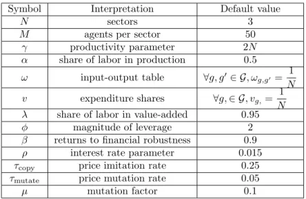
When these financial constraints are weak, i.e when the stock and the poten-tial inflow of capital in the economy is large with respect to the labor resources, the model has very robust properties of convergence to equilibrium. To illus-trate this point, we first consider a version of the model with three productive sectors (N = 3), fifty agents per sector (M = 50), and the remaining parameters set as in table 1 (in particular, the production network under consideration is symmetric). In this setting, the equilibrium price is equal to 1 for every good and the aggregate equilibrium production (resp. consumption) level is 100 (resp. 50). We initialize the model by drawing each price uniformly at random in [0, 2], allocating an initial wealth of 1 to each firm and of 100 to each bank. Then, resource constraints dominate as the equilibrium production level (100 units) is much less than what firms can finance without recourse to credit (300 units). Hence, as illustrated in the right panel of figure 1, total credit outstanding is negligible meaning that wages are mainly financed by firms’ net worth.
Con-straints on credit would anyhow be very weak: initial capital of banks is much greater than the recurrent financing needs of the production sector.
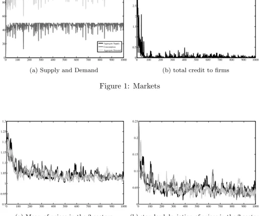
In this economy, the dynamics of the model are very clearcut: in about hundred periods, the mean private price of firms converges to its equilibrium value and the standard deviation of the price among firms become negligible (see figure 2) It is also the case that aggregate production and consumption reach their equilibrium values and that demand and supply balance each other (see left panel of figure 1). Hence the economy reaches equilibrium in approximately hundred periods and rests there for the remaining of the simulation.
0 100 200 300 400 500 600 700 800 900 1000 0 20 40 60 80 100 120 Aggregate Supply Consumption Aggregate Demand
(a) Supply and Demand
0 100 200 300 400 500 600 700 800 900 1000 0 0.5 1 1.5 2 2.5 3 3.5 4
(b) total credit to firms
Figure 1: Markets 0 100 200 300 400 500 600 700 800 900 1000 0.9 0.95 1 1.05 1.1 1.15 1.2 1.25 1.3
(a) Mean of prices in the 3 sectors
0 100 200 300 400 500 600 700 800 900 1000 0 0.05 0.1 0.15 0.2 0.25
(b) standard deviation of prices in the 3 sectors
Figure 2: Prices
To provide a quantitative assessment of the convergence properties of the model, we perform 250 Monte-Carlo simulations where we let the number of sectors vary from 2 to 6 and randomly draw 50 distinct production networks (the other parameters being set as in table 1). To assess the results of these simulations, we use a concept of approximate equilibrium:
Definition 2 The model is in an ✏-equilibrium in period t if:
1. The euclidian distance between the mean selling price and the equilibrium price is less than ✏;
2. The standard deviation of prices is less than ✏;
3. The excess demand (i.e total production minus total consumption minus total intermediary consumption as determined in 2.4. ) is less than ✏ times the total production.
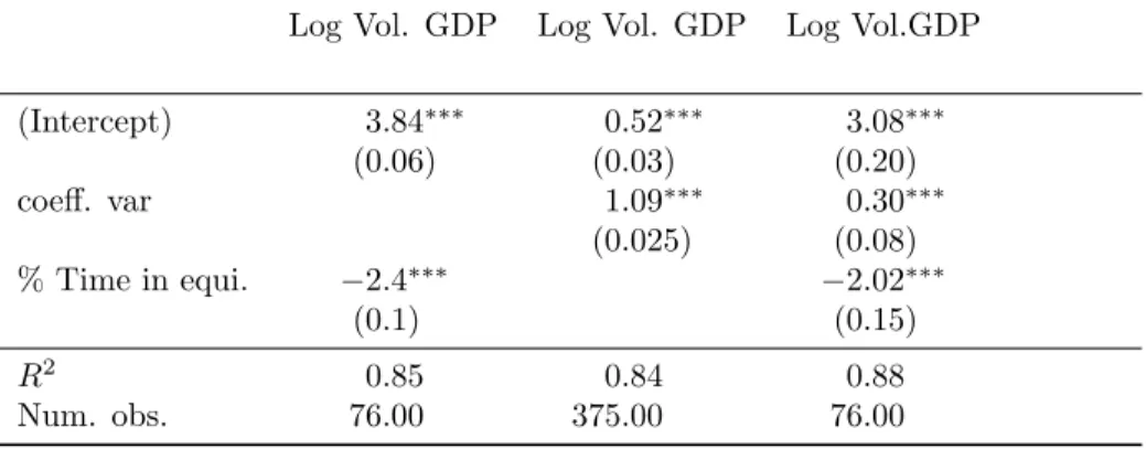
We then measure for the 250 Monte-Carlo simulations the mean number of periods in which the model is in an ✏-equilibrium (with ✏ = 0.1). The results are reported in table 2. Though the convergence time increases with the number of sectors, the model shows very robust properties of convergence to equilibrium. In the last 100 periods of the simulation, the model spends in average 80% of the time in equilibrium and for small number of sectors, the model is almost always in equilibrium.
# of sectors 2 3 4 5 6 mean
mean # of ✏-equilibria in periods 1-500 431 324 267 265 184 294
mean # of ✏-equilibria in periods 100-500 384 314 261 262 184 281
mean # of ✏-equilibria in periods 400-500 97 82 67 79 62 78
Table 2: nb of periods in equilibrium
Hence, we do obtain converge to equilibrium when resource constraints dom-inate. The small source of volatility introduced by the random mutations in the price formation process do not get amplified into aggregate volatility nor fragility. These good convergence properties are a first contribution of the model: we extend to an economy with intermediary production, the results of Gintis (2007) about the convergence to general equilibrium of private prices under evolutionary dynamics. It is worth noting in this respect that the intro-duction of efficient dynamics for the allocation of goods in 2.4 is perfectly in line with the axiomatic characterization of exchange processes inducing evolutionary stability of equilibrium obtained in Gintis and Mandel (2012).
3.3
Disequilibrium and financial fragility
The previous picture of economic equilibrium and financial stability seems at odds with the results reported in Delli Gatti et al. (2010) where “prices are important determinants of profits, which in turn a↵ect the accumulation of net worth and financial fragility. The financial vulnerability of an agent therefore is a↵ected by the dynamics of prices.”
Yet, the economic environment considered in Delli Gatti et al. (2010) is a particular case of ours with two sectors and intermediary consumption by
the second sector only, something that corresponds to ↵1 = 1, ↵2 = 0.5 and
! = ✓
0 0
1 0
◆
. The dynamics we consider are also very similar to these of Delli Gatti et al. (2010) but for the evolution of prices, which is purely random and exogenous in Delli Gatti et al. (2010) while it is endogenous and directed by evolutionary learning in our case. It is also the case that the sales of produced quantities at a purely random price in Delli Gatti et al. (2010) induce net inflows or outflows of money in the economy, whereas our model is stock-flow consistent as final consumption is entirely financed by wages and dividends.
One could therefore claim that it is the lack of stock-flow consistency and the exogenously imposed price volatility that induces financial fragility, network-based financial accelerator mechanisms, bankruptcy avalanches and aggregate volatility in Delli Gatti et al. (2010). We shall show this is not the case.
Indeed, even small shocks on the the price system induce variation in sales and profits and eventually in firms’ net worth. As soon as the financial con-straints are binding, downward variations in net worth lead to a decrease of pro-ductive capacity. Decreased capacity in turn lowers the competitive pressure, so that prices start leaving the equilibrium paths. Rationing and losses follow,
financial fragility increases and the way is paved for bankruptcy avalanches `a la
Delli Gatti et al. (2010).
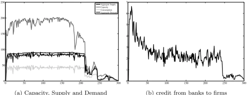
To illustrate this process, we consider a three-sector version of the model with parameters set as in Table 1 but where the initial net worth of firms is set equal to 0.25 and the one of banks equal to 2 (recall that these values also condition the capital of firms and banks created at runtime and hence the potential inflow of capital into the system). This economy is financially constrained, on the one hand because the aggregate production the firms can self-finance (75 units) is less than the equilibrium production (100 units) and on the other hand because the additional capital the banks can provide to the productive sector is also very limited. Indeed, as underlined in section 2.5.3, the only source of increase of the aggregate capital of the productive sector is the funding of new firms and the write-o↵ of the claims on bankrupt firms, which are both financed by the banks.
As illustrated in figures 3 and 4, the first hundred periods of the simulation are rather similar to the ones leading to equilibrium in section 3.2. A slight di↵erence being that in the very first periods, a series of bankruptcies induce a massive transfer of capital from the financial to the productive sector (see figure 5). It then seems that the productive sector reaches a level of capital compatible with the equilibrium production level. Yet this high capitalization is unsustainable as it is out of proportion with the financing flow that the financial sector can maintain towards the productive sector (see the right panel in figure 5). As a matter of fact, a shock to the price system around period 100 (see figure 4, most notably the right panel) triggers a temporary increase of the mean and of the standard deviation of the price of good 1, which induces a drop in demand (see figure 3) in sales, in profits and eventually in the net worth and
0 50 100 150 200 250 300 0 50 100 150 200 250 Aggregate Supply Capacity Consumption Aggregate Demand
(a) Capacity, Supply and Demand
0 50 100 150 200 250 300 0 1 2 3 4 5 6 7
(b) credit from banks to firms
Figure 3: Markets 0 50 100 150 200 250 300 1.05 1.1 1.15 1.2 1.25 1.3 1.35 1.4
(a) Mean of prices in the 3 sectors
0 50 100 150 200 250 300 0 0.05 0.1 0.15 0.2 0.25 0.3 0.35 0.4
(b) Standard deviation of prices in the 3 sectors
Figure 4: Prices 0 50 100 150 200 250 300 0 2 4 6 8 10 12 14 16 18 20
(a) Number of bankruptcies
0 50 100 150 200 250 300 0 20 40 60 80 100 120
(b) Bank wealths (Black) and Money Stock (Gray)
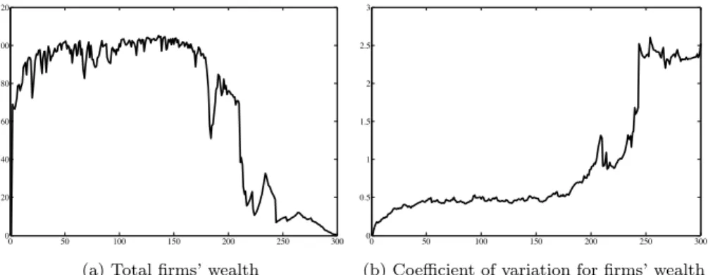
productive capacity of firms (see figure 6). Observing figure 5, one can remark that this loss of financial capital in the production sector is not compensated by a sizable inflow of capital from the financial to the production sector ; quite the contrary, the total net worth of banks is increasing. This is due to the fact that, as in Delli Gatti et al. (2010), the distribution of wealth among firms evolves during the simulation (see the evolution of the coefficient of variation in figure 6) and becomes much more dispersed. Larger firms face losses without going bankrupt and hence these losses are not passed to the financial sector (as it was the case at the beginning of the simulation when the size distribution of firms was uniform). Hence productive capacity does not recover, competition becomes less stringent and prices exit the equilibrium paths (see figure 4 from period 100 and onwards). As underlined in section 3.1, out-of-equilibrium, financial losses become structural. Consequently, the wealth of firm further decreases, interest rates increase with the financial fragility of borrowers and a positive feedback loop ensues which eventually leeds to a bankruptcy avalanche around period 170 (see figure 5). 0 50 100 150 200 250 300 0 20 40 60 80 100 120
(a) Total firms’ wealth
0 50 100 150 200 250 300 0 0.5 1 1.5 2 2.5 3
(b) Coefficient of variation for firms’ wealth
Figure 6: Firms’ wealth
The mechanisms at play are very similar to these described in Delli Gatti et al. (2010) “The bankruptcy of a borrower creates a negative externality because the bad debt recorded on the lender’s balance sheet yields an increase of the interest rate charged to all the other borrowers. This is the starting point of the financial accelerator. If the surviving borrowers experience an increase of leverage due to the interest rate hike, the lender will react by raising the interest rate even further. Financial fragility will spread to the neighborhood and may spill over to the entire economy. An avalanche of bankruptcies may ensue.” Yet, in our setting two other feedback mechanism are at play. First the decrease of financial capital and production capacity reduces the strength of competition and hence the stability of the price system. Second the sectoral interlinkages propagate rationing shocks throughout the system. These rationing shocks play the role of the idiosyncratic productivity shocks described in Acemoglu et al. (2012) as the drivers of aggregate volatility.
3.4
Financial constraints and phase transition
The simulations’ results reported above suggest that, depending on the strength of the financial constraints, the model exhibits two very di↵erent regimes. One is characterized by general equilibrium, low aggregate volatility and financial stability. The other is characterized by market disequilibrium, financial fragility and large aggregate volatility.
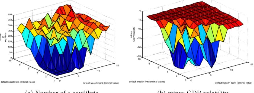
In order to test the assumption that financial constraints are the determi-nants of these two regimes, we run a series of 750 Monte-Carlo simulations (MC) where we let the default wealth of firms and banks vary (the other parameters being fixed as in table 1). More precisely, the default wealth of firms, which we denote by wf , takes the values (0.1250, 0.25, 0.4, 0.5, 0.6, 0.7, 0.8, 0.9, 1, 2), the one of banks, which we denote by wb, takes the values (0.5, 1, 1.25, 1.5, 1.75, 2, 2.25, 2.5, 3, 3.5, 4, 5, 10, 20, 50) and we run 5 MC over 500 periods for each possible combination of the variables wf and wb. Figure 7 provides a graphical illustration of the results by plotting, as a function of the default wealth of firms and banks, the mean (over the five MC) number of periods for which the model
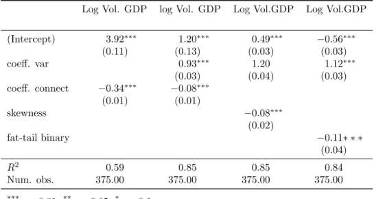
is in an ✏-equilibrium (with ✏ = 0, 1) and the mean volatility of GDP13.
0 5 10 15 0 2 4 6 8 100 50 100 150 200 250 300 350 400
default weakth bank (ordinal value) default wealth firm (ordinal value)
number ofequilibria
(a) Number of ✏-equilibria
0 5 10 15 0 2 4 6 8 10 −25 −20 −15 −10 −5 0
default wealth bank (ordinal value) default wealth firm (ordinal value)
minus
GDP volatility
(b) minus GDP volatility
Figure 7: Phase transition under financial constraints
The hypothesis that the financial constraints govern the regime of the model is confirmed by the identification of a phase transition between the equilibrium and the disequilibrium states of the model, which materializes as a critical line in the (wf, wb) plane. For small values of the pair (wf, wb) the model almost never is in equilibrium and exhibits high volatility, for large values of the pair (wf, wb) the model settles in equilibrium and exhibits low volatility. When the critical line is crossed, there is an abrupt transition between the two regimes. This abrupt transition between the two regimes can be well-approximated by a logistic function and suggests the existence of a phase-transition between equi-librium and non-equiequi-librium regimes. In this respect, our results are very similar
13The values on the x and y axis of figure 7 are ordinal, i.e 1 (resp. 15) corresponds to the
to those obtained in Gualdi et al. (2013): these authors show that phase tran-sitions between equilibrium and disequilibrium can be driven by small shifts in firms’ employment policy.
These results are robust with respect to change in the value of the other key financial parameter that is the interest rate. Additional simulations ran with a default interest rate varying between 0 and 6 percents yield a similar picture to the one presented in this section.
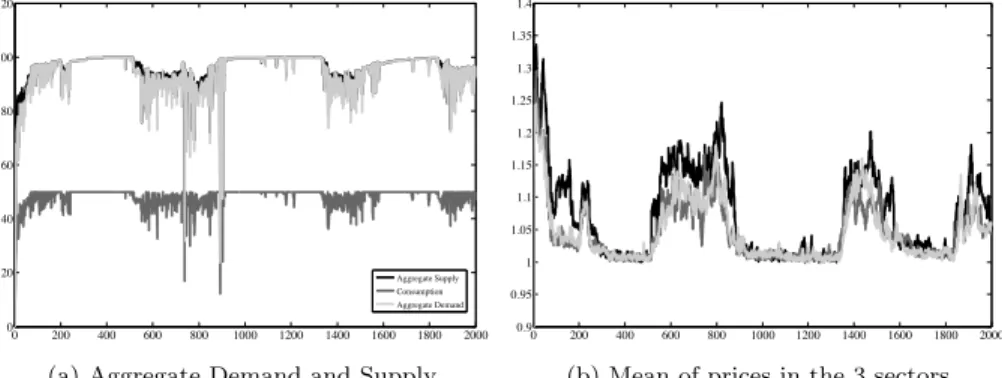
Additionally, we test the robustness of the results to changes in the dividend policy of the firm. The default financial policy of the firm is to distribute a dividend as soon as it makes a profit in the period (see 2.5.3). This very myopic behavior might be conductive to fragility as it prevents the firm from recon-stituting a strong enough capital basis after it has been a↵ected by a negative shock. In order to further investigate this point, we consider an alternative profit distribution policy which consists in distributing profits only if the current capi-tal of the firm is greater than a benchmark, which is set equal to the initial value of the capital. The use of this alternative financial management rule does not a↵ect the behavior of convergence to equilibrium reported in subsection 3.2 for parameter values that do not induce financial constraints. However in a setting with financial constraints, using the same parameter setting than in subsection 3.3, the results are qualitatively di↵erent (see figure 8). The model now exhibits shifts between an equilibrium regime where prices stay around their equilibrium value and aggregate volatility is very low, and a disequilibrium regime where prices fluctuate away from their equilibrium value and aggregate volatility is high. 0 200 400 600 800 1000 1200 1400 1600 1800 2000 0 20 40 60 80 100 120 Aggregate Supply Consumption Aggregate Demand
(a) Aggregate Demand and Supply
0 200 400 600 800 1000 1200 1400 1600 1800 2000 0.9 0.95 1 1.05 1.1 1.15 1.2 1.25 1.3 1.35 1.4
(b) Mean of prices in the 3 sectors
Figure 8: Markets
The main di↵erences with the processes that lead to collapse in section 3.3 is that the productive sector is now more resilient: bankruptcy crisis are less acute and the economy eventually recovers. This is due to the fact that firms now have time to recapitalize themselves after a shock.
Overall, one observes long-term fluctuations between an equilibrium regime characterized by stability of price and production and a disequilibrium one
![[PDF] Tutoriel de Présentation Ruby On Rails | Formation informatique](data:image/gif;base64,R0lGODlhAQABAIAAAP///wAAACH5BAEAAAAALAAAAAABAAEAAAICRAEAOw==)