Analysis of the Projective Re-Normalization method on semidefinite programming feasibility problems

Analysis of the Projective Re-Normalization Method on

Semidefinite Programming Feasibility Problems

by

Sai Hei Yeung

Submitted to the School of Engineering

in Partial Fulfillment of the Requirements for the Degree of

Master of Science in Computation for Design and Optimization

at the

MASSACHUSETTS INSTITUTE OF TECHNOLOGY

June 2008

©

Massachusetts Institute of Technology 2008. All rights reserved.

A uthor ...

....

...

..

...

...

School of Engineering

May 27, 2008

. . . ... ...

Robert M. Freund

Theresa Seley Professor in Management Science

A .

Thesis Supervisor

Accepted by ...

.... ...

.. . ... ... 3 ... ...

.. ... ...

Jaime Peraire

Professor of Aeronautics and Astronautics

Codirector, Computation for Design and Optimization Program

OF TEGHNOLOGY

JUN

112008

Certified by

...

.. .. ..

Analysis of the Projective Re-Normalization Method on

Semidefinite Programming Feasibility Problems

by

Sai Hei Yeung

Submitted to the School of Engineering on May 27, 2008, in Partial Fulfillment of the

Requirements for the Degree of

Master of Science in Computation for Design and Optimization

Abstract

In this thesis, we study the Projective Re-Normalization method (PRM) for semi-definite programming feasibility problems. To compute a good normalizer for PRM, we propose and study the advantages and disadvantages of a Hit & Run random walk with Dikin ball dilation. We perform this procedure on an ill-conditioned two-dimensional simplex to show the Dikin ball Hit & Run random walk mixes much faster than standard Hit & Run random walk. In the last part of this thesis, we conduct computational testing of the PRM on a set of problems from the SDPLIB [3] library derived from control theory and several univariate polynomial problems sum of squares (SOS) problems. Our results reveal that our PRM implementation is effective for problems of smaller dimensions but tends to be ineffective (or even detrimental) for problems of larger dimensions.

Thesis Supervisor: Robert M. Freund

Acknowledgments

I would like to express my deepest gratitude to my thesis advisor, Professor Robert

M. Freund. I will miss our research meetings where he taught me so much about the subject of convex optimization. The research methodologies he instilled in me will be invaluable in any career I choose to pursue in the future.

I would also like to thank Alexandre Belloni, who provided me with valuable insights on my research, many of which became important elements to my final thesis. Furthermore, I would also like to thank Professor Kim Chuan Toh, who generously took time out of his busy schedule to provide me with insight on the computational testing section of this thesis. Thanks also goes to Laura Koller, who provided me with so much help from getting me an office space to sending me reminders about various due dates that I was sure to forget otherwise.

I have made many new friends during my two years at MIT. I would like to thank

them for keeping me sane and optimistic when the pressures from exams or research bogged me down. They include members of the MIT Lion Dance Club, members of the Hong Kong Students Society, Eehern Wong, Catherine Mau, Kevin Miu, Leon Li,

Leon Lu, Shiyin Hu, Rezy Pradipta, Daniel Weller, and James Lee.

Thanks to Aiyan Lu and Howard Wu for always being there for me and making my transition to Cambridge an easy one. Finally, thanks to my brother Sai To and my parents Chiu Yee and Sau Ping for their unconditional love and support. I dedicate this thesis to them.

Contents

1 Introduction 13

1.1 M otivation . . . . 13

1.2 Thesis O utline . . . . 17

2 Literature Review and Preliminaries 19 2.1 Re-Normalizing F by Projective Transformation . . . . 19

2.2 Semidefinite Programming and Polynomial Problems . . . . 21

2.2.1 N otation . . . . 21

2.2.2 Semidefinite Programming Introduction . . . . 22

2.2.3 Sum of Squares Problems and SDP . . . . 24

3 Computing a Deep Point 27 3.1 Standard Hit & Run Random Walk . . . . 28

3.2 Improving the Hit & Run Random Walk . . . . 31

3.2.1 Dikin Ball Hit & Run Random Walk . . . . 32

3.2.2 Performance Analysis on a Two-Dimensional Simplex . . . . . 37

3.2.3 Performance Analysis for Higher Dimensions . . . . 40

4 Computational Tests 43

4.1 Test Set-U p . . . . 43

4.1.1 Problems from SDPLIB Suite . . . . 43

4.1.2 Initial Conditions . . . . 45

4.1.3 Geometric measures of the system . . . . 49

4.1.4 Testing Overview . . . . 49

4.2 Results & Analysis . . . . 51

4.2.1 Improvement in number of iterations . . . . 51

4.2.2 Improvement in running time in SDPT3 . . . . 53

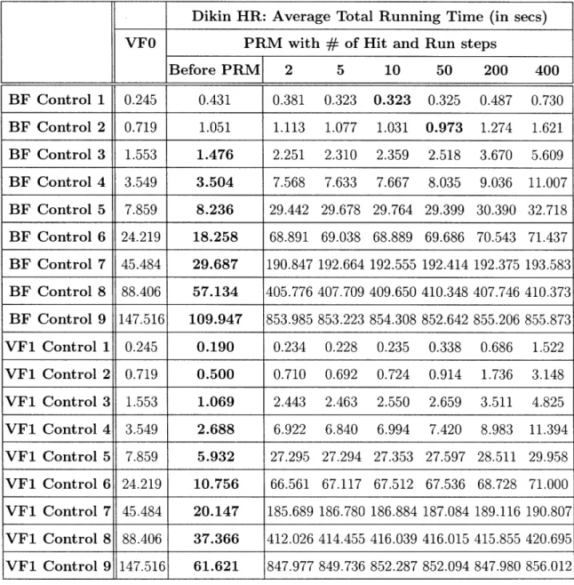
4.2.3 Improvement in total running time . . . . 57

4.2.4 Analysis of 6* . . . . 58

4.3 Tests on Ill-Conditioned Univariate Polynomial Problems . . . . 62

4.3.1 Test Set-Up . . . . 62

4.3.2 Results & Analysis . . . . 63

4.4 Summary of Results . . . . 65

5 Conclusion 67

List of Figures

3.1 Mapping between H and (H ) ...

3.2 Iterates of Standard H&R over Simplex . . . . 3.3 Iterates of Dikin ball H&R over Simplex . . . . 3.4 Standard vs. Dikin ball H&R: Convergence to Center of Mass of the Sim plex . . . . 3.5 Mobility of Standard H&R Iterates . . . . 3.6 Mobility of Dikin H&R Iterates . . . .

Running Time vs. Running Time vs. Running Time vs. Running Time vs. Running Time vs. Running Time vs. Running Time vs. Running Time vs. Running Time vs.

Number of Hit & Number of Hit & Number of Hit & Number of Hit & Number of Hit & Number of Hit & Number of Hit & Number of Hit & Number of Hit &

35 38 38 39 41 42 6.1 6.2 6.3 6.4 6.5 6.6 6.7 6.8 6.9 Control 1: Control 2: Control 3: Control 4: Control 5: Control 6: Control 7: Control 8: Control 9: Run Steps Run Steps Run Steps Run Steps Run Steps Run Steps Run Steps Run Steps Run Steps . . . . . 69 . . . . . 70 . . . . . 71 . . . . . 71 72 . . . . . 72 . . . . . 73 . . . . . 73 . . . . . 74

List of Tables

4.1 Size and primal geometric measure of our test problems. . . . .4 4.2 Using Standard H&R:

over 30 trials... 4.3 Using Dikin-ball H&R:

over 30 trials. . . . . 4.4 Using Standard H&R: 30 trials . . . . 4.5 Using Dikin-ball H&R:

30 trials . . . . 4.6 Using Standard H&R:

trials . . . .

Average number of iterations to reach feasibility

Average number of iterations to reach feasibility

.. A.ver . .D...

...

n.n .. .

...

.f.e..

. ....

Average SDPT3 running time to feasibility over

Average Total Running Time (in secs) over 30

4.7 Using Dikin H&R: Average Total Running Time (in secs) over 30 trials 4.8 Time (in seconds) for the Dikin ball computation at the origin of HT

and time of an IPM step. The values for an IPM step time are the average over iterations of one run . . . . 4.9 0* values for BF before PRM vs. BF after PRM (using 100 Standard

Hit & Run steps) . . . . 52 54 55 56 59 60 61 61 44

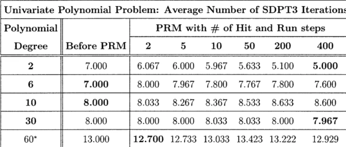
4.10 Univariate polynomial problems: Average number of iterations to reach feasibility over 30 trials. For UP of degree 60, the results are averaged over successful trials only. . . . . 63

4.11 Univariate polynomial problems: Average SDPT3 running time over

30 trials. For UP of degree 60, the results are averaged over successful

trials only. . . . . 64 4.12 Univariate polynomial problems: Average total running time over 30

trials. For UP of degree 60, the results are averaged over successful trials only. . . . . 64 4.13 Univariate polynomial problems: 0* values for BF before PRM vs. BF

Chapter 1

Introduction

1.1

Motivation

We are interested in the following homogeneous convex feasibility problem:

(1.1)

F:

Ax=O

X

E C

\

where A E L(R", ]R') is a linear operator and C is a closed convex cone.

When we assign C <- K x JR+, A <- [A, -b], and consider only the interior of C, we see that F contains the more general form of the conic feasibility problem:

Ax =

b

x E K.

Definition 1. Given a closed convex cone K C R, the (positive) dual cone of K is

Now consider a point 9 E intC*. It is easily seen that the following normalized problem: Ax =0 F T = 1 (1.3) x E C, is equivalent to F.

The image set of Fg, denoted by Hg, is

Hg:= {Ax:,§Tx = 1,x E C}. (1.4)

Definition 2. Let S C R' be a convex set. The symmetry of a point t in S is defined as follows:

sym(, S) := max{tly E S -> t - t(y - t) E S}. (1.5)

Furthermore, we define the symmetry point of S as follows:

sym(S) := max sym(i, S). (1.6)

tES

Definition 3. Let C be a full-dimensional convex subset of Rn. A function f : intC -+

R is called a V -self-concordant barrier for C with complexity value V if f is a barrier

function for C and the following two conditions hold for all x E intC and h E Rn:

" V3f(x)[h, h, h] 2(V 2f(x)[h, h})3/2.

"

In [2], Belloni and Freund show that the computational complexity and geometric behaviour of F can be bounded as a function of two quantities: the symmetry of the

image set Hg about the origin, denoted as sym(O,H), and the complexity value O of the barrier function for C. Here, computational complexity of F refers to iteration bound of an interior point method (IPM) for solving F.

Let the relative distance of x from the boundary of C, denoted as

C,

reldist(x,1C) :

dist(x,C)

and define the width rF of the feasible region F = {x : Ax = 0, x E C} as:

TF = max{reldist(x, aC)} = max {reldist(x, aC)}. (1.8)

x EF Ax=O,xEC\{O}

We say that F has good geometric behavior if the width -rF of the cone of feasible solutions of F is large. This occurs when F has a solution x whose reldist(x,

C)

large.

Given 9 E intC*, there is a natural norm 11 - || on Rn associated with 9, see [2] for details. This norm has certain desirable properties, one of which is stated in the following theorem.

Theorem 1. [2] Let 9

E

intC* be given. Under the norm

1|g, the width rF of F

satisfies:

(1)

sym(0, Hg)

sym(0, Hg)

(1.9)

Vi

1 + sym(O, Hg) ~~

1 + sym(O, Hg)

In particular, -sym(0, H)

sym(O,

Hence, given an image set H that is perfectly symmetric about the origin (i.e., sym(0, Hg) = 1), the width rF of the feasible solutions cone is guarenteed to be larger than '

To motivate the complexity result, we consider an optimization model that solves

Fg. Let § E intC* be chosen and assign ± +- -Vf*(9), where

f*(,§)

bar-rier function on C* evaluated at 9. Then ± E C, and we construct the following optimization problem:

(OP) :t* := min 0

s.t. Ax - (A±) = 0 (1.10)

sTx

x E

C.

Note that (x, 9) = (., 1) is feasible for (OP) and any feasible solution (x, 9) of OP

with 9 < 0 yields a feasible solution J = (x - 0±) of F. We can now summarize the

computational complexity result in the following theorem:

Theorem 2. [2] Let 9 E intC* be chosen. The standard short-step primal-feasible interior-point algorithm applied to (1.10) will compute ± satisfying Ai = 0, - E intC

in at most

sym(0, Hg)

iterations of Newton's method.

Theorems 1 and 2 are the main driving forces behind this thesis. In the subsequent chapters, we build on these two theorems as we explore strategies to improve geometry and computational performance of semi-definite programming feasibility problems.

1.2

Thesis Outline

In Chapter 2, we provide background on the Projective Re-Normalization (PRM) method and semi-definite programming. Chapter 3 presents the two main methods of obtaining "deep" points in a convex set: the Standard Hit & Run random walk and the Dikin ball Hit & Run random walk. In Chapter 4, we present formulation and results of computational tests performed to analyze our methods. Chapter 5 concludes the thesis with a summary and a discussion of future work.

Chapter 2

Literature Review and

Preliminaries

2.1

Re-Normalizing F by Projective

Transforma-tion

The dependence of the computational complexity and geometric behaviour of F§ on sym(0, Hg) leads us to consider improving sym(O, Hg) by replacing 9 with some other

c

Ax =

0

Tx _{= 1}

X C C,

with the modified image set:

Hg ={Ax : x E C,

sJX

(2.1)

However, checking membership in Hg is difficult. (Just the task of checking that 0 E Hg is as hard as solving F itself.)

Definition 4. Given a closed convex set S C Rd with 0 E S, the polar of S is S' := {y E Rd : yTX < 1 for all x E S}, and satisfies Soo = S.

Let us consider the polar of the image set H,'. It can be shown that H. = {v E

Rm : 9 - ATv E C*}, see [2].

From [1], it is shown that for a nonempty closed bounded convex set S, if 0 E S, then sym(O,S) = sym(0,SO), which suggests the possibility of extracting useful information from H,. Working with H. is attractive for two reasons: (i) by the choice of 9 E intC*, we know 0 E H.0 and (ii) as we shall see, the Hit & Run random

walk is easy to implement on Hg.

A look at H.0 shifted by 0 E intH reveals the identity expressed in the following theorem.

Theorem 3. [1] Let 9 E intC* be given. Let 0

E

s :=-ATb . Then

sym(0, Hs) = sym(0, H,')

Theorems 1, 2, and 3 suggest that finding a point 0 E H,, with good symmetry can yield a transformed problem Fg with improved bounds on TF and IPM iterations.

In this thesis, we will call points x in which sym(x, S)

>

We can turn this into an overall improvement in the original normalized problem Fg with the following one-to-one mapping between Fg and Fj via projective transfor-mations:

X' < and x <- . (2.3)

x _ST

As the reader may expect, the pairs Hg and Hg are also related through projective transformations between y E Hg and y' E Hg:

y' = T(y) :- and y=T- 1(y') - .

1 - 1y 1+ )Ty

(2.4)

We now formalize the procedure in the following algorithm:

Projective Re-Normalization Method (PRM): Step 1. Construct H' := {v E R' : 9 - ATv E C*}.

Step 2. Find a suitable point 'L E H. (with hopefully good symmetry in H,) Step 3. Compute . := 9 - AT

Step 4. Construct the transformed problem: Ax =0

Fg: {Txz= 1 _(2.5)

Step 5. The transformed image set is H := {Ax E JR" : x E C , Tx = 1}, and sym(0, Hg) = sym(D, H,).

2.2

Semidefinite Programming and Polynomial

Prob-lems

2.2.1

Notation

Let S" denote the space of n x n symmetric matrices. For a matrix M E S', M >- 0 and M -< 0 means that M is positive definite and negative definite respectively, and

M > 0 and M -d _{0 means that M is positive semi-definite and negative semi-definite,} respectively.

For two real matrices A E R"'f and B E R' x" , the trace dot product between A

and B is written as A * B = E"

Z

2.2.2

Semidefinite Programming Introduction

A semidefinite programming problem (SDP) is expressed in its primal form as

minx C . X

s.t. Ai * X = bi, i = 1 ... m (2.6) X > 0,

or in its dual form as

maxy bTy (2.7)

s.t. (yiAi -- C

i= 1

Here, Ai, C, and X E S', and y and b E R'm.

Definition 5. In the context of problems (2.6) and (2.7), X is a strictly feasible primal point if X is feasible for (2.6) and X >- 0, and y is a strictly feasible dual point if y is feasible for (2.7) and

>'l

It is easy to observe that the feasible region of an SDP, either in its primal or dual form, is convex and has a linear objective, hence is a convex program. Because

of convexity, SDPs possess similar duality properties seen in linear programming problems. In particular, weak duality holds for all SDPs while strong duality holds under some constraint qualifications such as existence of strictly feasible points. The duality result can be summarized in the following theorem:

Theorem 4. [10] Consider the primal-dual SDP pair (2.6)-(2.7). If either feasible region has a strictly feasible point, then for every e > 0, there exist feasible X, y such

that C - X - bT y < e. Furthermore, if both problems have strictly feasible solutions,

then the optimal solutions are attained for some X,, y*.

The parallels between linear programming problems and SDP's extend to al-gorithms. Along with convexity and duality properties, the existence of a readily computable self-concordant barrier function allows the possibility of interior point method (IPM) algorithms for SDP's. In fact, Nesterov and Nemirovsky show in [9] that interior-point methods for linear programming can be generalized to any con-vex optimization problem with a self-concordant barrier function. Extensive research in algorithm development has led to very efficient IPM-based SDP solvers such as SDPT3 [12].

SDPs arise in many problems in science and engineering. The most important classes of convex optimization problems: linear programming, quadratic program-ming, and second-order cone programming can all be formulated as SDPs. In engi-neering, SDPs often arise in system and control theory. In mathematics, there exist

SDP formulations for problems in pattern classification, combinatorial optimization,

and eigenvalue problems. [14] provides an extensive treatment of SDP applications. For a rigorous treatment of the theory of SDP, refer to [13]. We next look at a particular application of SDP.

2.2.3

Sum of Squares Problems and SDP

Non-negativity of a polynomial f(x) is an important concept that arises in many prob-lems in applied mathematics. One simple certificate for polynomial non-negativity is the existence of a sum of squares (SOS) decomposition:

f(x) = E fi (x). (2.8)

If a polynomial f(x) can be written as (2.8), then f(x) > 0 for any x.

In some cases, such as univariate polynomials, the existence of SOS decomposi-tion is also a necessary condidecomposi-tion. But in general, a nonnegative polynomial is not necessarily a SOS. One counter-example is the Motzkin form (polynomial with terms of equal degree):

M(x, y, z) =x4y2 + x 2y4 + z6 -3x 2 2z2

. (2.9)

Checking for existence of SOS can be posed as an SDP. Consider a polynomial

f(x

less than or equal to d. Notice the dimension of z is (nfd. _n!d! We claim that

f

Q

f(x) = zTQz, Q >- 0. (2.10)

satisfies (2.10). Since

Q

Q

rewrite (2.10) as

f(x) = zTLT Lz = |ILz12= Ei(Lz)2. (2.11)

Here, the terms of the SOS decomposition are (Lz), for i = I... rank(Q).

The formulation of (2.10) as an SDP is achieved by equating coefficients of mono-mials of f(x) with that of zTQz in expanded form. The resulting SDP in primal form is

{Q

0,

For example, consider the polynomial

f(x) = X2 - 2x + 1.

This polynomial can be written in the form of

f

(x)=

[

a

bl

I,

with identities a = 1, 2b = -2, and c = 1.

1 0 A, =

0 0

]

The problem of checking non-negativity of a polynomial f(x) can be extended to other applications. One such application is global minimization of a polynomial (not necessarily convex) which can be formulated as the following SOS problem:

max _y

s.t. f(x) - y is SOS, (2.17)

which can be transformed into an SDP. (2.12) with

(2.15)

Chapter 3

Computing a Deep Point

From the previous chapter, we learned that the origin of the image set Hg :=

{Ax:

-Tx = 1, x E C} has good symmetry if it has good symmetry in the more accessible

polar set H, = {v E R' : § - ATv E C*} as well. To perform projective

re-normalization on H, we first need a deep point in the set. One way to obtain this point is by repeated sampling on the polar image set H,. Because this set is convex, the Hit & Run random walk is a suitable sampling method.

Consider the following optimization problem:

(BF): 0* := min 0

s-t. Ai * X -

X -0, X2 ;> 0.

= 0, i=l ... m (3.1) = 1

Observe that (BF) has a structure very similar to (OP) and solves the feasibility problem in the form (1.2), so long as x2 > 0.

T and t are initially set to I and 1 respectively prior to re-normalization. X and

Z2 are set to 9 _and ' respectively. Note that T - T-' = n where n is the rank of

n+1 n+1

T, and hence 0 1, X = XX 2 = Z2 is feasible for (BF).

The corresponding image set HTf and its polar image H ,, are

HTj

:=

T

Hp',j:= {v E Rm : T -

_{viAi -,}

_-

_{vi(-b) > 0}.}

i=1 i=1

3.1

Standard Hit & Run Random Walk

The Hit & Run (H&R) random walk is a procedure to sample points from a uniform distribution on a convex set. We give a formal description of this procedure below in the context of sampling on the polar image set H .

We next describe how to compute the boundary multipliers [03, OU]. Procedure 3.1: Standard Hit & Run over H

Given Hg, described in (3.3).

Step 1. Start from a feasible point v = v, in the convex set.

Step 2. Randomly sample a direction d from the uniform distribution on the unit sphere.

Step 3. Compute boundary multipliers [i,/3], defined as follows:

# min{t E R : v + td E H } (3.4)

1%= max{t E R : v + td E H } (3.5)

Step 4. Choose a uniformly on the interval [0i1, IO]. Step 5. Update v: v = v + ad.

Procedure 3.2: Computing boundary multipliers

Given direction d, and current iterate v.

Step 1. Compute boundary multipliers for half-space (Min-Ratio Test): Step la. Initialize /3i= -o0, /3u = 00, e = tolerance

Step 1b. Set N = (f+ bTv) and D = bTd,.

" If INI < e and/or IDI < e, set N = 0 and/or D = 0 respectively.

e If D > 0 and -N/D > /3i', then updateO11i, = -N/D. " If D < 0 and -N/D <,3u, then update /3u = -N/D.

Step 2. Compute boundary multipliers for semi-definite inequalities: Step 2a. Compute G T - I" vjAj and K = - E>(di)A'.

Step 2b. Compute the minimum and maximum generalized eigenvalues, Amin and Amax, of K with respect to G. This involves solving for the generalized eigenvalue-eigenvector pairs {(Ai, Xi)},=1., defined as solutions to the following system:

Kxj = AXGxj. (3.6)

Step 2c. Set !3DP 1/Amax and ISuDP 1/Amin

Step 3. Set /3 = max{J3₁'n, OSDP} and 3u = min{/3in, O3uDP}.

In our tests, we use the MATLAB 7 .0 function eig () to compute Amin and Amax.

A special property of the Hit & Run random walk is that it simulates a Markov

chain and the sampling of points converges to the uniform distribution on the set. The rate of convergence to this distribution depends on the difference of the two largest eigenvalues of the transition kernel of the Markov Chain. We point the reader to [8] for a comprehensive analysis of the Hit & Run algorithm and its complexity.

As a result of this property, the sample mean of the iterates converges to the center of mass y of the set, which is very likely to have the "deepness" property that we look for in a normalizer, since for a bounded convex set S E R" we have

sym(pu, S) > 1/n. We can use the sample mean of the iterates in this procedure to

projectively re-normalize our image set.

3.2

Improving the Hit & Run Random Walk

A fundamental flaw with using the standard Hit & Run random walk to sample a

convex set appears when we investigate the iterates near a tight corner. The iterates tend to be immobile and bunch up in the corner for a very large number of iterations before escaping. It is easy to imagine that at any tight corner, a large proportion of directions obtained from random sampling on the unit ball would lead to boundary points near this very corner, preventing escape into deeper points of the convex set. The problem increases dramatically as the dimension increases, since the difficulty of escaping a bad corner increases.

With this problem in consideration, we can immediately think of two ways to resolve the problem. One is to perform a transformation of the convex body so that the corner is no longer as tight by expanding the walls surrounding the corner. Another is to transform the unit ball such that the direction is chosen from a distribution with higher probabilities on directions pointing away from the corner. Both of these ideas suggest using information about the shape of the convex set.

To motivate our idea, we first introduce the Lowner-John theorem:

set S, provides a V\-rounding of S when S is symmetric and an n-rounding of S

when S is not symmetric.

This theorem gives us the idea of using an ellipsoid to approximate the shape of a given convex set. One such ellipsoid is that defined by the sample covariance matrix of the convex set. In fact, we can form bounds on the volume of the convex set using two ellipsoids based on the covariance matrix, as seen in the following theorem developed in [7] through ideas from the Lowner-John theorem and [8]:

Theorem 6. [7] Let X be a random variable uniformly distributed on a convex body

S c J'. Then

BE (p, '(d + 2)/d) c S c BE (p, d(d + 2)) (3.7)

where p denotes center of mass of S and E denotes the covariance matrix of X, and

BE(x,r) denotes the ball centered at x with radius r in the norm | : vTE-1v.

Using the sample covariance matrix to get an approximation of the local shape of the convex set sounds like an attractive idea. However, the integrity of the approxi-mation depends highly on how well the sample points represent the local shape. As we later show, using standard Hit & Run from a corner may produce poor sample points.

To resolve this problem, we can explore the use of local shape information given

by a self-concordant barrier function for H g.

3.2.1

Dikin Ball Hit & Run Random Walk

Denote F(v) = T - E' v2A2. We now define a suitable self-concordant barrier

#(v) = - log(i+ bv) - log det F(v).

The gradient of this function at v is

(V())= -b

+

Tr[F(v)~1Ai],

(3.9)

Vt+

and the Hessian at v is

(V2(V))= ( bT)2ib

+ Tr[F(v)-'AiF(v)~

Aj],

(3.10)

The gradient and Hessian of the part of (v) corresponding to semi-definite in-equalities (the second terms of (VO(v))i and (V2

0(v))ij) are derived from its Taylor

series expansion. We direct the reader to [131 for a complete derivation.

We now define a mathematical object that is central to our strategy to approximate the local shape of our feasible region.

Definition 6. Let

f(.)

Bv(v, 1) := {y :

IIy

vJo,

A property we are interested here is self-concordance, which has the physical interpretation that variations in the Hessian of the self-concordant function between two points y and v are bounded (from above and below) by the distance between y and v measured in the norm 11 - 11v or 11 - ||y. For a more extensive treatment of (3.8)

self-concordant functions, we point the reader to [9] or [11].

Stemming from self-concordance, the Dikin ball defined by the Hessian of the barrier is known to be a good approximation of the local structure of the convex set at a given point. The following theorem captures this fact.

Theorem 7. [9] Given a convex set S, and a V0-self-concordant barrier 0(.) for S

and its gradient Vq(-), for any point v E S, the following is true:

Sn {d: VO(v)Td > O} C B,(v, 30 + 1). (3.12)

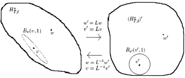
Because of this property, we seek to use the Dikin ball to improve our Hit & Run iterates. In particular, we can dilate the set Hp,, we wish to sample from with the Dikin ball at v E H , via the transformation {w': w' E (Hpf)'} = {Lw : w E Hp,,},

where V2

0(v) = LTL. Figure 3.1 illustrates the mapping between the spaces of H',F

and its transformation (H.,g)'.

From the figure, we see the Dikin ball maps to the unit ball under the transfor-mation. Hence, sampling from the unit ball in the transformed space corresponds to sampling from the Dikin ball in the original space. We now give the formal procedure of the Dikin ball Hit & Run random walk.

/H

=

/ =

L-

Figure 3.1: Mapping between H? and (H )'

The boundary multipliers are calculated as described in Procedure 3.2.

The steps in the procedure provide a general framework for sampling over a set. The computation of the Hessian can be very expensive, hence updates of the scaling factor should be kept to a minimum in order to optimize overall performance. In particular, Step 3 and 4 of the procedure should only be done when necessary (i.e., when the last computed Dikin ball is no longer a good approximation of the local region of the set).

Procedure 3.3: Dikin ball Hit & Run over H

Given H1 described in (3.3) and its barrier function (3.8).

Step 1. Start from a feasible point v = vo in the convex set H .

Step 2. Randomly sample a direction d from the uniform distribution on the unit sphere.

Step 3. Compute V2

q(v), the Hessian of the barrier function at v.

Step 4. Compute the Cholesky factorization of the positive-definite matrix V2

0(v)

= LT L.

Step 5. Compute the new direction d'= L d.

Step 6. Compute boundary multipliers [3, 0,,], defined as follows:

# min{t E R : v + td' E H } (3.13)

max{t E R: v + td' E H } (3.14)

Step 7. Choose a uniformly in the interval [13, O].

Step 8. Update v: v = v + ad.

3.2.2

Performance Analysis on a Two-Dimensional Simplex

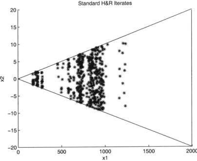
The two-dimensional simplex is chosen for our initial test for two reasons: (i) the ease of plotting allows us to visually compare the iterates using Standard Hit & Run versus Dikin ball Hit & Run, and (ii) the center of mass p of a two-dimensional simplex is easy to compute. Here we consider a two-dimensional simplex defined by the vertices (0, 0), (2000, -20) and (2000, 20). This is clearly a very badly scaled convex region. The center of mass, p of this set is simply the mean of the three vertices, which is (4000/3,0).

We perform 500 Standard H&R and Dikin ball H&R steps over the simplex start-ing at (X1, x2) = (200, 0). For the test of Dikin ball H&R, the Dikin ball, computed

at the starting point (X1, x2) = (200, 0), is used to sample our directions from at each

step of the random walk. Figures 3.2 and 3.3 show the resulting plots. Note the large contrast in resolution between the x1 and x2 axes.

Note that majority of the iterates are jammed near the left corner when Standard H&R is used. This is not surprising since Standard H&R uses the Euclidean ball to uniformly select a direction and only a small proportion of these directions (those that are close to parallel with the xi-axis) would allow it to escape the corner. The Dikin-ball scaled H&R avoids this problem as it chooses its direction uniformly over the Dikin-ball, which tends to produce directions somewhat parallel to the s1-axis.

Observe the distribution of iterates is more uniform over the simplex with the Dikin H&R.

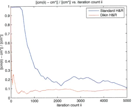
Figure 3.4 plots the normalized error of the approximate center of mass at step i of the H&R, cm(i) =

4

Standard H&R Iterates 20- 15- 10- 5-x 0l 20 -5--10 -15-0 500 1000 1500 2000 x1

Figure 3.2: Iterates of Standard H&R over Simplex

Dikin H&R Iterates

2015

-10

15 - *# **

xx

Figue 33: Ieraes Diin AllHRoe ipe

I1cm(ii) - cm*| / I1cm*1I vs. iteration count ii 1 Standard H&R 0.9 Dikin H&R 0.8 0.7-E -0.6 -E 0.5-0.4 0.3 0.2 0.1 0 1000 2000 3000 4000 5000 iteration count ii

Figure 3.4: Standard vs. Dikin ball H&R: Convergence to Center of Mass of the

Simplex

less than 300 steps to get within 10% of p. The latter requires more than 1500 steps to get within 20% of p and it does not get closer than 10% even with 5000 steps. Also note that the cm(i) values of the Dikin ball H&R stabilizes very early whereas it is unclear whether the cm(i) values of Standard H&R have stabilized after 5000 steps.

3.2.3

Performance Analysis for Higher Dimensions

While the analysis of the algorithm performed on a two-dimensional simplex conve-niently demonstrates the idea of the Dikin-ball Hit & Run random walk, it does not necessarily translate to effectiveness of the method on general convex sets of higher dimensions.

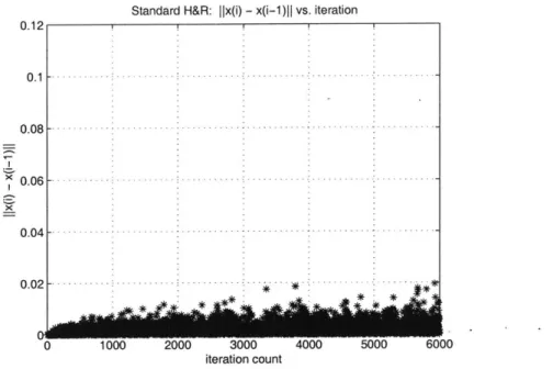
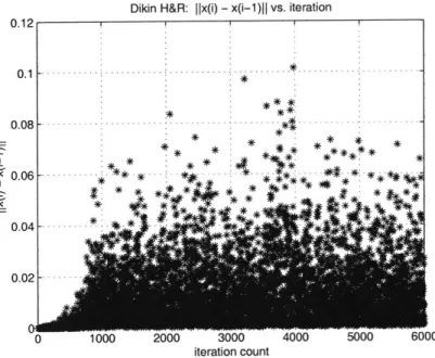
In a higher dimensional convex set S with semi-definite inequalities, neither the center of mass cm nor the symmetry function sym(x, S) can be computed easily. Visualization of the iterates in the manner of the previous section is also not possible. Instead, we can observe the behavior of the random walk by plotting the norm of the differences between successive iterates. Figures 3.5 and 3.6 plot the successive iterate difference norms,

Ilx(i

Observe that the difference between successive iterates is very small when Stan-dard H&R is used, implying the random walk mixes very slowly. The average absolute difference between iterates is 0.002 when Standard H&R is used and 0.011 when Dikin ball H&R is used, larger than the former case by more than a factor of 5. While we cannot conclude whether convergence to the center of mass is faster for Dikin ball H&R, we believe that the Dikin scaling allows greater mobility of the iterates within the convex set.

Standard H&R: ||x(i) - x(i-1)I vs. iteration 0.12 0.1 - -0.08 - : - --0.04 - -0.02 . . 0 1000 2000 3000 4000 5000 6000 iteration count

Figure 3.5: Mobility of Standard H&R Iterates

3.2.4

Boundary Hugging & Warm-Start

We performed trials of the Dikin ball H&R with the Dikin ball updated at every iteration. What we observed was that when an iterate gets sufficiently close to the boundary, the Dikin balls start morphing to the shape of the boundary and become increasingly ill-conditioned. The stretched ellipsoids tend to yield subsequent iterates that stay close to the boundary, leading to a random walk that "hugs" the boundary. Hence it is desirable that we compute our Dikin ball from a point that is not too close to the boundary. A simple heuristic for getting this point is to warm-start with standard Hit & Run iterations until we obtain a satisfactory point away from the boundary before calculating the Dikin Ball.

Dikin H&R: I|x(i) - x(i-1)|I vs. iteration

.

.

Figure 3.6: Mobility of Dikin H&R Iterates

42 0.12 0.1 0.08 -.. x 0.06-0.04- -0.02

-Chapter 4

Computational Tests

4.1

Test Set-Up

In [2], computational tests were performed to validate the practical viability of the projective re-normalization method on linear programming feasibility problems. Here, we extend this work to semi-definite programming feasibility problems. The results from the computational tests that follow give us further insight to the Projective Re-normalization Method (PRM) on SDPs as well as the Dikin Ball scaled Hit & Run random walk.

4.1.1

Problems from SDPLIB Suite

We use a subset of problems from the SDPLIB library of semi-definite programming problems [3]. These problems derive from system and control theory and were con-tributed by Katsuki Fujiwasa [6].

Table 4.1 contains information on size and geometry of the problems we use to conduct the computational tests. The problems when expressed in the standard

pri-Table 4.1: Size and primal geometric measure of our test problems.

mal SDP form (2.6) have m linear equalities, each with constraint matrices Ai of size

n x n. These SDP problems are all feasible and have similar constraint matrix

struc-tures. The gp values in Table 4.1 provide us with a measure of geometric properties of the primal feasible region. A formal definition of 9P follows. See [4] for information on how the gp values are computed.

Definition 7. [4] For a primal SDP of form (2.6), we define the primal geometric measure gp to be the optimal objective function value of the optimization problem:

g mnxmax

lixil_

gP X

IIXII

OS", ")

5

For further discussion on this set of problems, refer to [6]. To provide the reader greater intuition on the testing that follows, we include the structure of the these problems below.

Let P E RI"L,

Q

maxS,D,A

-pTS _ SP

-

-SQ

-QT S

D

S >- AI,

where the maximization is taken over the the diagonal matrix D = diag(di, d2, ... , dk),

the symmetric matrix S E S"xL, and A E R. The problem can be re-written in the form of the standard dual SDP (2.7) with m =

1(1

In this form, we notice the resulting problems would have a 2-block matrix structure with block dimensions of (1 + k) x (1 + k) and

1

4.1.2

Initial Conditions

For optimal computation performance, it is desired that we start our algorithm near the central path, defined by the minimums of the barrier function parameterized by the barrier coefficient p. In our tests on the optimization problem (BF) (3.1), we provide SDPT3 a feasible starting point that is close to the central path of the

primal-dual space. We generate this point by solving a system of equations to satisfy primal feasibility, dual feasibility, and a relaxed central path condition. Here we provide a brief outline of how to generate this point. Consider the conic dual of (BF):

max.,s, ₂ s.t. M

Zr

A +TS+S - 0

E1r(-AX +

Combining the primal and dual constraints with a relaxation of the central path condition, we form the following system of equations for the central path.

Central Path Equations:

As

9[A

X

Zi iriAi + 6 + S =0

(4.7)

Zi

S

f

(4.12)

Notice that (4.11) is equivalent to !X/ 2_SX/ 2 _{I = 0. To obtain a point that is}

close to the central path, we replace (4.11) and (4.12) with the following simultaneous relaxation:

4 where 11 -

IIy

Definition 8. For a matrix M and a scalar a,

1IM, a||y

(4.14)

where |IMI|F is the Frobenius norm.

such that (4.4) - (4.10) and (4.13) are satisfied.

Let 7r be the solution of the following quadratic program:

min, r / + (Z ibif2)2 (4.15)

i=1

s.t. 7r(-Ai e f

+

i=1

We can rewrite the problem in the following form:

min, 7rTQ7r (4.16) s.t. q T 7r where

Qjj

We then set /pt =

4 max{iI

E

IF

>2_

7ribi-Mi respectively.

It is easy to see that with the above assignments, (4.4)-(4.9) are satisfied. (4.10) is satisfied if (4.13) is true. The key to verifying (4.13) is by substituting S =

-

Z

!X/2SX1/2 _

IrXI/

and

11 m

A25-21 = Z ribif2, (4.21)

We can then take the appropriate norms on both sides to arrive at the result.

4.1.3

Geometric measures of the system

Unlike the case of polyhedra, there is no known efficient way to determine how asym-metric the origin is in a system involving semi-definite constraints such as H;,,, the polar image set of (BF). We discussed in Chapter 2 the difficulty of computing the symmetry function for this type of system. Despite this, we can use heuristic methods to find certificates of bad symmetry in the system. One simple way is to check cords that pass through the origin of the set. The symmetry of the origin along a cord provides an upper bound on the symmetry of the origin in the entire set. We will see later that the optimal objective value 0* of (BF) also provides information on the geometry of the set. In particular, 0* provides an upper bound on the symmetry of the origin with respect to H;,, (i.e., sym(0, Hpot) <; *).

4.1.4

Testing Overview

In order to test the practicality of the PRM method, it is necessary to compare our results using the (BF) formulation of the feasibility problem with that of the generic

non-homogeneous versions of the feasibility problem. We will consider two formula-tions below, which we call "Vanilla Feasibility 0" (VFO) and "Vanilla Feasibility 1" (VF1): minx (VFO) s.t. minx (VF1) s.t.

0.x

For (VFO), we allow SDPT3 to determine the starting iterate internally. For (VF1), we set the initial iterate to X0 = -T , y, = [0..0]T, and ZO T. For (BF) and

(VF1), we conducted our tests both without PRM (hence the normalizer T >- 0 is the

identity matrix I, and f is 1) and with PRM for a set of different Hit & Run steps values. Both Standard Hit & Run and Dikin ball scaled Hit & Run were used to compute the deep point for PRM. Their performance are then compared. The results for (BF) and (VF1) are the averages over 30 trials for each experiment. We solved (VFO) and (VF1) to primal feasibility and (BF) for 0 < 0, the criteria that implies

feasibility of the original problem.

GB DDR2 RAM, and a 40 GB 7200RPM SATA hard drive.

4.2

Results & Analysis

We discuss the results on different performance measures for solving (BF) after PRM on the set of Control problems. We compare these measures to those of three cases:

(i) (BF) before PRM, (ii) (VFO), and (iii) (VF1).

4.2.1

Improvement in number of iterations

Table 4.2 summarizes our computational results on the number of SDPT3 iterations required to attain feasibility when Standard H&R is used for PRM. Notice for all the problems, the number of iterations generally decreases with more Hit & Run steps. This is expected as a larger number of Hit & Run points will yield a better approximation to the center of mass, which we expect to yield a better normalizer for PRM. When the best result is compared to (BF) before PRM is applied, we see significant improvement of more than 33% for smaller dimensional problems (Control 1 to Control 3) and modest improvements for medium sized problems (Control 4 and Control 5) of almost 20%. Similar improvements are seen when compared to (VFO) and (VF1) before PRM.

We note that improvement in iteration count is limited for the problems with larger dimensions. When compared to (BF) before PRM, two problems, namely Control 7 and Control 8, actually took more iterations on average after re-normalization with a small number of Hit & Run steps. When compared to (VF1) before PRM, problems Control 6 through Control 9 all take longer even with 400 H&R iterations. Problems of higher dimension tend to take a much larger number of H&R steps to reach reasonably

Standard HR: Average Number of SDPT3 Iterations

VF0 PRM with

#

Before PRM 2 5 10 50 200 400 BF Control 1 10.000 8.000 8.067 7.500 6.833 5.900 5.800 5.633 BF Control 2 11.000 10.000 9.931 10.172 9.483 7.724 7.345 7.655 BF Control 3 11.000 10.000 10.000 10.333 10.467 9.667 8.000 7.467 BF Control 4 11.000 10.000 11.000 11.167 11.500 10.967 9.667 8.767 BF Control 5 11.000 11.000 11.000 11.433 11.600 11.100 9.767 8.967 BF Control 6 12.000 12.000 11.900 12.033 12.233 11.800 11.133 9.800 BF Control 7 12.000 11.000 11.000 11.733 11.967 11.600 10.200 10.100 BF Control 8 12.000 11.000 11.333 12.433 13.033 12.233 11.100 10.333 BF Control 9 12.000 13.000 13.100 13.000 13.333 12.767 12.333 11.900 VF1 Control 1 10.000 9.000 8.500 7.500 7.033 4.667 4.200 4.233 VF1 Control 2 11.000 9.000 8.967 9.000 8.933 7.767 6.500 6.033 VF1 Control 3 11.000 9.000 9.333 9.567 9.733 8.533 7.100 6.300 VF1 Control 4 11.000 10.000 9.600 9.567 9.567 9.200 7.933 7.000 VF1 Control 5 11.000 10.000 10.000 9.933 9.967 9.767 8.800 7.700 VF1 Control 6 12.000 9.000 9.533 9.767 9.967 9.600 9.000 8.433 VF1 Control 7 12.000 9.000 9.000 9.200 9.300 9.167 9.000 8.300 VF1 Control 8 12.000 9.000 9.133 9.667 9.833 9.833 9.000 9.000 VF1 Control 9 12.000 9.000 9.433 9.633 9.900 9.733 8.733 8.933 Table 4.2: Using Standard H&R: Average number of iterations to reach feasibility over 30 trials.

deep points, which may explain the poor performance of these problems.

Looking at the (VF1) data, the reader may notice a decrease in iteration count for all the problems as more H&R steps is used. For Control 1, when compared to

(VFl) before PRM, an improvement of almost 50% is seen with 200 H&R iterations. It is known that the performance of the primal-dual interior-point method used in

SDPT3 is very sensitive to the initial iterates. In particular, one seeks a starting

iterate that has the same order of magnitude as an optimal solution of the SDP and is deep within the interior of the primal-dual feasible region. It is curious for these problems that deep points within Hp would yield good initial iterates. The same procedure may yield very poor initial iterates for a different problem.

Table 4.3 summarizes our computational results on the number of SDPT3 itera-tions required to reach feasibility when Dikin-ball H&R is used for PRM. Small but considerable improvement on iteration count of the best case is observed over the case of Standard H&R for problems Control 1 and Control 3. A small increase in iteration count for Control 2 is observed when compared to the Standard H&R case. No significant difference between the two cases is seen for the other problems.

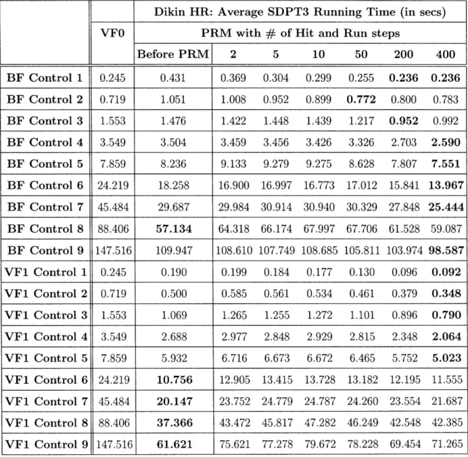
4.2.2

Improvement in running time in SDPT3

Table 4.4 summarizes the average SDPT3 running times of each test when Standard H&R is used to compute the normalizer. The values do not include the time taken in the Hit & Run algorithm itself. The results complement our iteration count analysis. As with iteration count, when compared to (BF) before PRM, we see improvement in SDPT3 running time with more H&R steps. Also, we see the improvement factor is greater for the problems with smaller dimensions. When compared to (VFO), the best result of (BF) is worse for Control 1 but becomes increasingly better with the

Dikin HR: Average Number of SDPT3 Iterations

VFO PRM with

#

Before PRM 2 5 10 50 200 400 BF Control 1 10.000 8.000 7.567 6.400 6.300 5.467 5.000 5.000 BF Control 2 11.000 10.000 9.900 9.433 8.967 7.800 8.167 8.000 BF Control 3 11.000 10.000 10.100 10.300 10.233 8.733 7.000 7.267 BF Control 4 11.000 10.000 11.000 11.033 10.967 10.667 8.800 8.467 BF Control 5 11.000 11.000 11.000 11.000 11.033 10.567 9.333 9.000 BF Control 6 12.000 12.000 11.900 11.967 11.833 11.967 11.200 10.000 BF Control 7 12.000 11.000 11.000 11.300 11.300 11.100 10.267 9.433 BF Control 8 12.000 11.000 11.433 11.900 12.167 11.967 11.067 10.533 BF Control 9 12.000 13.000 13.067 12.967 13.067 12.733 12.567 11.933 VF1 Control 1 10.000 9.000 8.667 8.167 7.700 6.233 4.567 4.833 VF1 Control 2 11.000 9.000 9.000 8.933 8.933 7.800 6.667 6.033 VF1 Control 3 11.000 9.000 9.300 9.567 9.667 8.467 7.033 6.267 VF1 Control 4 11.000 10.000 9.700 9.367 9.600 9.267 7.867 7.000 VF1 Control 5 11.000 10.000 10.000 9.967 9.967 9.633 8.700 7.700 VF1 Control 6 12.000 9.000 9.467 9.833 10.033 9.667 9.000 8.567 VF1 Control 7 12.000 9.000 9.000 9.367 9.367 9.167 8.933 8.300 VF1 Control 8 12.000 9.000 9.200 9.667 9.967 9.733 9.033 9.000 VF1 Control 9 12.000 9.000 9.433 9.633 9.900 9.733 8.733 8.933 Table 4.3: Using Dikin-ball

over 30 trials.