An analysis of oil supply disruption scenarios

(1)

AN ANALYSIS OF OIL SUPPLY DISRUPTION SCENARIOS

Knut Anton Mork

MIT Energy Laboratory Report No. MIT-EL-81-010 April 10, 1981

(2)

1. Introduction and Summary

This report brings the results of simulations of some oil supply disruptions on the M.I.T. Energy Laboratory Energy Macro Model. This model has previously been used to study the macroeconomic effects of the 1973-74 and 1979 oil price shocks, as well as for policy simula--tions related to these historical events (Mork and Hall, 1980a, 1980b,

1981). Recent extensions of the model allow it to be used for simula-tion of possible future oil supply disrupsimula-tions, such as the loss of oil deliveries from Saudi Arabia or the entire Persian Gulf region.

The extensions go mainly in the direction of more explicit modeling of thedomestic energy sector and of the world oil market. Although very important, these extensions are still in an experimental stage. Richard Gilbert of the University of California at Berkeley provided invaluable help in modeling the domestic energy sector. The short-run functioning of the world oil market was modeled along the lines suggested by Chao and Manne (1980). Sanjay Srivastava provided useful research assistance in preparing and programming the solution algorithm for the model. None of these persons are, however, in any way responsible for

the contents of this report.

Three basic disruption scenarios are analyzed, of 3, 10, and 18 million barrels per day (mmbd) on the world level, respectively.

Disrup-tions are modeled as leftward shifts in the world supply curve for oil (OPEC's 'price reaction' curve). All disruptions are assumed to last for one year, but another three years are assumed to be needed to restore the lost capacity. Each disruption scenario is simulated under three

(3)

different policy assumptions. The first case assumes no new policy. The second case assumes a specific tariff on oil imports, rising from $2.50 in 1981 to a long-run value of $10.00 in 1984. In the third case, an ad valorem tariff is introduced gradually in the same way, from 7.5 percent of the world price in 1981 to 30 percent in 1984. As a last exercise, a 10 mmbd disruption is simulated under the assumption that all relative prices adjust perfectly to clear all markets.

Oil supply disruptions are found to add substantially to inflation during the disruption year and to cause substantial real losses. For a 10 mmbd disruption (the possible loss of Saudi Arabia), 6.4 percentage points are expected to be added to the inflation rate in the disruption year, and the net social cost in real terms is projected as $489 billion

in 1980 dollars. An 18 mmbd disruption (the possible loss of the Persian Gulf) is expected to lead to an 8 percent drop in real GNP in the year of the disruption, to add 14 percent to the inflation rate and 6.5 percent to the unemployment rate in the same year, and to incur a net loss of $1,010 billion in 1980 dollars.

The two tariffs are found to lead to very similar results. The ad valorem tariff may hold a slight edge over the specific tariff by

reducing transfer the real income to oil exporters during a disruption by slightly more than it increases the loss due to unemployment. Both tariffs are, however, clearly inferior to the alternative of no new policy because of the added losses and inefficiencies in normal periods.

If all prices and wages were free to adjust instantaneously, so that full employment were maintained everywhere during a disruption, then the

(4)

3

world oil market would be.much higher and the price increase more than three times as high. This effect of unemployment on oil prices provides an automatic stabilizer in the world market and is an important part of the explanation of the apparent resilience of the U.S. economy to large disturbances in the world oil market.

(5)

2. The Model

The model used is an extended version of the model presented by Mork and Hall (1980b). This section outlines the changes and extensions relative to that version.

Domestic Energy Supply

The most important change is that the supply of energy is modeled explicitly rather than treating its price as exogenous. Domestic supply of aggregate energy is modeled according to the theory of ex-haustible resources. Domestic firms are assumed to take the price of energy as given. The cost of extraction is given by the marginal cost function

cE(R,S,t) = eAt c RV + c2 e- p S (1)

where R is the extraction rate, S the resource stock, t is time, and cl , c2, v, p, and A are parameters. v decreases over time.

Its value is very high in the early periods, so that the marginal cost of extraction beyond a critical level (1/cl) quickly becomes very high. This formulation approximates short-run capacity limits and gives a very low short-run supply elasticity.

As energy resources are extracted over time, marginal extraction cost increases. This is reflected in the second term of (1), which makes the marginal cost curve shift vertically. A leftward shift

seems reasonable as well, reflecting reduced extraction capacity when the stock is decreased. This effect is approximated by a multiplica-tive time trend in the first term. The trend formulation was chosen

(6)

OMMii uIYh.,

5

because it is easier to solve dynamically than a formulation with an explicit multiplicative dependence on S.

By excluding relative prices, (1) assumes implicitly that a homo-geneous good (the output of the goods and service sector) is the only input to energy extraction. By avoiding labor and capital in the energy sector as explicit variables, this formulation facilitates greatly the numerical solution of the model.

The assignment of parameter values for the energy sector is based on similar principles as the rest of the model. Rather than estimating each parameter from time series data, such values have been picked as give reasonable projections. R is measured in 1972 billion dollarrs (at 1972 energy prices). cl is chosen so as to give a realistic

initial value of R. v declines from 25 in the disruption year to a long-run value of 4 from the 6th year after the disruption. x and p equal 0.077 and 0.007, respectively. The value of c₂serves only to set a scale for S, as will be seen below. Its actual value, 1012, has no independent meaning.

Dynamic programming implies the following arbitrage condition for domestic energy supply:

r(P-c) = E - (ac/aR)k - (ac/av) - ac/at , (2)

where PE is the real price of energy, r the real interest rate, and dots denote time derivatives. In the solution of the model, r is taken from the solution of the goods and service sector, and the time

(7)

derivatives are approximated by forward-looking first differences. A producer tax or subsidy can easily be added to (2).

The model assumes a backstop price FE. Extraction does not stop immediately when this price is reached, but continues until the rent (price minus marginal cost) becomes zero at zero extraction.(1) Thus, the terminal stock S is defined implicitly by the condition

e-p

PE c ePS E - 2 or = (1/p) _kn(c 2/PE)

The initial resource stock S_O(in 1980) is assumed to be such that the marginal extraction cost is one eighth of the market price. Thus,

S ₀ = (1/p) zn[c₂_{/(P/8)] .} 2

The solution of the model uses the transversality condition that total extraction equals the difference between So and S:

JR(t)dt = So - = (1/p) kn(8CE/P). 0

(1)The backstop technology is used in the model only eventually. Over-shooting of the backstop price can occur in earlier periods, for example, as the result of a supply disruption.

(8)

Since c₂does not enter in this condition, its value is inessential for the solution.

With the marginal cost function (1) in a continuous-line model, extraction approaches zero only approximately. For the discrete approximation used here, extraction is "cut off" when it becomes

suf-ficiently low. The time of cut-off is determined by simple discrete search.

Oil Import Supply

The world oil market is modeled by a simple static import supply curve or price reaction function for the first six years of the solu-tion. For the remaining period, the world price of oil is assumed to follow a constant-growth path (2 percent annual real increase) until the backstop price is reached. The import supply curve is modeled along the lines suggested by Chao and Manne (1980). It consists of two parts. First, OPEC pricing is assumed to follow the price reaction curve

Po = c+ , (3)

0 k-Q

where Po is the real world price of oil, k is OPEC capacity, and Q is world demand for OPEC oil. The parameters c and d are chosen so that the world price for 1980 is $35 per barrel and the marginal cost of oil for the non-OPEC world,

P, = P + Q

(9)

equals $65 for 1980.

A disruption is modeled by modifying (3) as

P = c + (l-)d, (3')

S( - )k-Q

where e is the disruption in percent of OPEC capacity. Obviously, an increase in E shifts the price reaction curve to the left along the Q-axis.

It should be emphasized that the static price reaction curve is a very crude way of modeling the behavior of OPEC's members. The curve represents, at best, a short-run relationship. Thus, we may

expect the price reaction curve to shift in response to policy.

Determination of oil import supply for the United States also re-quires a model of non-U.S., non-OPEC demand. This is modeled by postulating a simple aggregate production function for real non-energy output of these countries:

YF = [A(-)/o+(B(RF+MF))(-1)/]/(-) , (4)

where YF is output, RF is energy supply by these countries, and MF their demand for imported oil. RF is assumed exogenous. The elasti-city of substitution a rises over time from 0.04 in the disruption year to a long-run value of 0.4 after 6 years. The parameter values A and B are determined so that actual prices and input and output

(10)

-- mIYIII~I.II

9

po = B(a-l)/a [YF/(RF+MF) /o . (5)

The parameter A is a proxy for capital and labor inputs. During a disruption, the model adjusts this parameter to conform with the relative reduction in U.S. input levels. In other words, other • countries are assumed to experience the same recession as the United States. Needless to say, this phenomenon softens the world oil market considerably during a disruption. On the other hand, when the model simulates offsetting macro-economics policies, only domestic input

levels are assumed to respond directly, so no adjustment is made in the value of A.

Domestic energy demand for the United States is derived from the model of the goods and service sector. U.S. import demand is then determined as the difference between demand and domestic supply. World demand, Q, is taken to be the sum of U.S. and foreign import demand. The model can then be solved for the world price of oil, P . This price is translated into the aggregate price of energy by the assump-tion that any oil price increase above the level of the baseline solu-tion leads to a change in the overall price of energy of 80 percent of

the oil price increase. A tariff is easily added to this formulation. Short-run Technology

Another new feature approximates a putty-clay technology and

gives a very low demand elasticity for energy in the short run. Essen-tially, the model assumes fixed coefficients between energy and

capital in the short run, while substitution may take place over time.

(11)

This feature comes in addition to the quasi-fixity of capital in the short run.

The technology is described by a unit cost function. This cost function now has the form

1(w/P,v,PE) = [(w/Pv,PE)]g[n(w/PvPE)1-g _, (6)

where w is the nominal wage rate, P is the overall price level, and v the real rental price of capital. is the long-run, or ex ante, cost function described in the previous publication. n is the short-run, or ex post cost function, with the form

n(w/P,v,PE) = yo[av+ (1 -a)PE l-a (w/P)a . (7)

The parameters yo, a, and a are computed from prices and input combina-tions that the model predicts if no shock occurs. The weight g in (6) rises over time from 1/6 in the disruption year to a long-run value of 1 after 6 years.

Price and Wage Determination

The overall price level is determined as a weighted geometric average of the market-clearing price level P and a contract or admin-istered price P, which is a fixed mark-up over variable cost:

^a -1-a

P P P (8)

(12)

S= _{n(w,Pv,PPE) ,}

where a is a weight increasing over time from 0.25 in the disruption year to a long-run value of I after 4 years. The fixed mark-up v is the mark-up that would clear the market in the absence of a disruption. The previous version used a similar formulation, only v was then taken as the post-disruption long-run value of the mark-up. This change makes little difference for the analysis of oil supply disruptions, but has substantial consequences for the projected price level effects of monetary policy.

A slight modification was also made in the indexation of the com-mitted wage rate w. The lag in the indexation process has been

removed, so the formulation used now is

w* = Wl + y(P-P)/P] ,

where P is the price level expected in the absence of a disruption. This change was made only for the purpose of avoiding the wage rate as a state variable with an initial condition, which would have compli-cated the backward solution method of the model. The backward solution

is convenient for the two-point boundary problem implied by the model because it-avoids the numerical instability which marred the previous,

forward solution algorithm.

On the other hand, evidence of a lag is found in the data and is easily rationalized as an information lag. As an approximation to

(13)

the empirical evidence, the parameter y is taken to be 0.25 in the disruption year and 0.5 thereafter. Since an oil supply disruption results pretty much in a once-and-for-all change in the price level, this formulation is actually very close to one with an explicit lag. Gross National Product and Consumption

Since domestic energy extraction uses real resources, the distri-bution of real non-energy output is changed to

Y = C + I + Z + X + G , (12)

where C is consumption, I is investment, X is net exports of non-energy goods, G is government expenditure, and Z is resources devoted to energy extraction. From (1), Z is defined as

Z = CE(R',S,t)dR' = ( )eAt R + + c2e-pS . (13) cE+ 1 2

Since the model now includes the domestic energy sector, it can compute total Gross National Product (GNP). This is defined as the sum of value added in the two sectors.

GNP = Y-PEE+PER- Z = Y-PEM-Z (1) (14)

where E and M are domestic energy demand and energy import demand, respectively.

(In _{the actual computation, oil imports is evaluated at the price of} oil, not the price of aggregate energy. Also, note that double deflation is not used in the computation of GNP.

(14)

Since this version of the model accounts consistently for all resource use of the domestic economy, it can be used for cost-benefit analysis. Given the life-cycle, permanent-income formulation of con-sumer behavior presented in the earlier publication, the initial level of consumption can be used as a unique indicator of social welfare. The net social cost of any event can be estimated as the discounted sum of changes in consumption over time.

Consistent use of this criterion requires, however, an explicit modeling of the real payment for imported oil, that is, the exchange of non-energy exports for imported oil. Empirically, oil exporters seem willing to accept various kinds of claims on the U.S. economy as temporary payment and seem likely to cash in these claims for U.S. goods only gradually and over time. In the model, this is reflected by allowing the trade balance to be in deficit. However, it is balanced in the long run by assuming that the discounted value of net exports of non-energy goods equals the discounted value of present and future oil imports. The model is then closed by assuming that oil exporters will spread their purchases evenly over time indefinitely, in the sense

that net exports of non-energy goods will grow over time at the same rate as domestic consumption.

I_ IIIII IIIIIYIIY

(15)

--3. Disruption Scenarios Without a Tariff

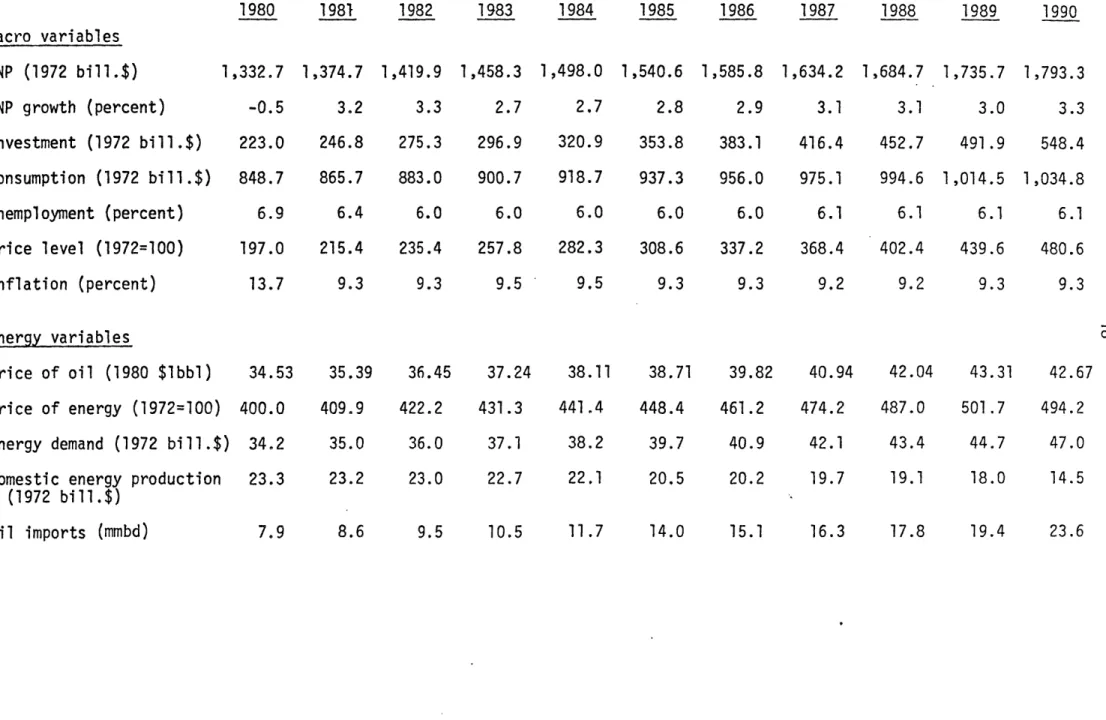
The first task needed for this analysis was to construct a baseline projection, showing the likely course of the economy in the absence of oil supply disruptions and new policy. This baseline projection is pre-sented in Table 1. It should be emphasized that this projection is not meant to be a forecast; its only purpose is to serve as a basis for com-parison.

The projections for 1980 deviate somewhat from the published pre-liminary data. Typically, real variables are lower and the price level

higher in the projection than in the data. This is mainly due to a

difference in convention. In the published GNP data, each item is deflated separately. Obviously, the relative price of imports (including oil)

has increased substantially since 1972. Then, since imports are sub-tracted off in the computation of GNP, this procedure gives a much higher value of real GNP than if nominal GNP as a whole had been deflated by a broad-based price index for finished goods. The model uses the latter procedure and deflates all nominal variables by the price of gross output of the goods and service sector. Since all primary energy is used as

inputs to the goods and service sector in the model, this price index includes energy used by consumers, such as gasoline and electricity. It has been calibrated to correspond to the Consumer Price Index.

The model assumes no productivity growth and 2 percent annual growth in the labor force. The relatively high long-run real growth rate

(around 3 percent) is due to the projected real increase in energy prices over time. The expectation of rising energy prices provides an

(16)

incentive to save now for the worse times ahead.

The experimental character of the energy sector of the model should be emphasized. For example, the lagged effect of price decontrol on domestic supply is not accounted for. Even apart from this, the decline rate for domestic energy production may be too high.

Since policy is to be introduced in the model in 1981, while disrup-tions are assumed to occur unexpectedly in 1985, the construction of the base case caused a slight technical problem. Since the model assumes rational expectations, a scenario with a future shock and policy manipu-lation before the shock requires the running of two versions of the model. In the present case, the two versions start in 1980 and 1985, respective-ly. Policy is introduced in the 1980 version without expectation of the future shock. The 1985 version must in turn include the effect of policy on those state variables that do not jump, in this case, the capital shock and the domestic resource shock. The baseline projection

is put together from these two versions, both run without any shock. The synchronization is quite close, but a slight discontinuity for domestic energy production (and hence imports) between 1984 and 1985 is noticeable.

Tables 2-4 show the projected results of oil supply disruptions of 3, 10, and 18 million barrels per day (mmbd) on the world level, respec-tively. Each disruption is assumed to last for one year; however, I assume that it takes another three years before the disrupted capacity is restored.

(17)

The pattern of effects is very similar in the three disruption scenarios. GNP declines dramatically in the first year. Then it re-bounds to some extent but stays at a lower level permanently. The per-manent loss is due to the slowing of capital formation during the

recession. Since the model does not deflate each GNP component sepa-rately, the GNP loss includes the partial effect on real income of the higher import bill. This effect would not be reflected directly in the published GNP data.

Unemployment follows the pattern of GNP, but gets back to its normal level after three or four years. The course of the price level is

interesting: It rises dramatically in the year of the disruption. It declines thereafter relatively to its previous path, but very slightly, and it stays at a substantially higher level permanently. The higher permanent level is mainly the result of the reduced level of real output: the same supply of money is being chased by fewer goods. In terms of inflation rates, this path is.described as a large one-shot increase followed by a near-zero effect.

The larger disruptions have, of course, larger effects. And the increase is progressive. For the effect on consumption as well as first-year GNP, the loss per barrel disrupted rises with the size of the disruption.

The effect on oil prices may seem small. The reason is that the disruption-induced recession softens the demand for oil in the United States as well as in other countries. This automatic stabilizer in the oil market is the explanation why an 18 mmbd disruption is not quite as

(18)

The tables only give price increases in real terms. Effects of increases in inflation on nominal prices come on top of this.

It should be noted that the price projections are for annual averages. In the even shorter run, oil prices may,.of course, go sub-stantially higher. It may also be noted that speculative behavior in the oil market is reflected in the model only in the supply of domestic energy, which is highly inelastic. But even if speculative buyer

behavior were modeled explicitly, it would not have added to the price increase because all agents are assumed to expect that the disruption will be over quite soon. The speculative behavior observed in 1979, which seemed to contribute substantially to the dramatic price increase, must have been based on a different expectation.

The slight decline in oil prices in 1988 and 1989 occurs because the permanent decline in production levels lowers the demand for oil. The model assumes that the price reaction curve does not move in re-sponse to this decline. On the other hand, a return back to normal oil prices from 1990 is imposed on the solution of the model. While a

return to normal conditions seems reasonable, it may happen more abruptly in the model than in the real world.

The model permits computation of the total social cost of each dis-ruption as the discounted value of the reduction in aggregate consumption. In 1972 dollars, this is given as $60 billion, $248 billion, and $513

billion, respectively, for each of the three disruption sizes. In 1980 dollars, the corresponding figures are $119 billion, $489 billion, and $1,010 billion, respectively.

(19)

Table 1 Baseline Projection 1980 1981 1982 1983 1984 1985 1986 1987 1988 1989 1990 Macro variables GNP (1972 bill.$) 1,332.7 1,374.7 1,419.9 1,458.3 1,498.0 1,540.6 1,585.8 1,634.2 1,684.7 1,735.7 1,793.3 GNP growth (percent) -0.5 3.2 3.3 2.7 2.7 2.8 2.9 3.1 3.1 3.0 3.3 Investment (1972 bill.$) 223.0 246.8 275.3 296.9 320.9 353.8 383.1 416.4 452.7 491.9 548.4 Consumption (1972 bill.$) 848.7 865.7 883.0 900.7 918.7 937.3 956.0 975.1 994.6 1,014.5 1,034.8 Unemployment (percent) 6.9 6.4 6.0 6.0 6.0 6.0 6.0 6.1 6.1 6.1 6.1 Price level (1972=100) 197.0 215.4 235.4 257.8 282.3 308.6 337.2 368.4 402.4 439.6 480.6 Inflation (percent) 13.7 9.3 9.3 9.5 9.5 9.3 9.3 9.2 9.2 9.3 9.3 Energy variables Price of oil (1980 $lbbl) 34.53 35.39 36.45 37.24 38.11 38.71 39.82 40.94 42.04 43.31 42.67 Price of energy (1972=100) 400.0 409.9 422.2 431.3 441.4 448.4 461.2 474.2 487.0 501.7 494.2

Energy demand (1972 bill.$) 34.2 35.0 36.0 37.1 38.2 39.7 40.9 42.1 43.4 44.7 47.0

Domestic energy production 23.3 23.2 23.0 22.7 22.1 20.5 20.2 19.7 19.1 18.0 14.5

(1972 bill.$)

Oil imports (mmbd) 7.9 8.6 9.5 10.5 11.7 14.0 15.1 16.3 17.8 19.4 23.6

(20)

TAble 2

3 mmbd World Oil Supply Disruption in 1985, No Tariff Projected Deviations From Baseline Projection

1985 1986 1987 1988 1989 1990

Macro variables

GNP (1972 bill $) -28.4 -16.8 -12.0 -10.2 -8.2 -10.1

GNP growth (percentage points) -1.2 0.8 0.3 0.1 0.2 -0.1

Investment (1972 bill $) -22.6 -14.4 -11.6 -10.6 -8.2 -10.0

Consumption (1972 bill $) -3.6 -3.7 -3.8 -3.8 -3.9 -4.0

Unemployment (percentage points) 0.7 0.2 0.1 0.0 0.0 0.0

Price level (percentage change) 1.1 1.2 1.1 1.0 1.0 1.0

Inflation (percentage points) 1.3 0.0 -0.1 -0.1 -0.1 -0.1

Energy variables

OPEC capacity shortfall (mmbd) 3.00 2.25 1.50 0.75 0.00 0.00

Price of oil (percentage change) 9.8 5.4 2.1 -0.2 -1.5 0.0

Price of energy (percentage change) 7.8 4.4 1.7 -0.1 -1.2 0.0

Energy demand (1972 bill $) -0.7 -0.8 -0.6 -0.4 -0.2 -0.3

Domestic energy production 0.3 0.3 0.2 0.1 -0.1 _0.1

(1972 bill $)

(21)

Table 3

10 mmbd World Oil Supply Disruption in 1985, No Tariff Projected Deviations From Baseline Projection

1985 1986 1987 1988 1989 1990

Macro variables

GNP (1972 bill $) -121.2 -64.3 -45.3 -40.3 -34.0 -41,1

Investment (1972 bill $) -99.5 -55.9 -43.4 -40.8 -33.1 -40.4

Consumption (1972 bill $) -14.8 -15.1 -15.4 -15.7 -16,0 -16.3

Unemployment (percentage points) 3.0 0.7 0.2 0.1 0.0 0.0

Price level (percentage change) 5.2 5.2 4.8 4.5 4.3 4.1

Inflation (percentage points) 5.7 -0.0 -0.3 -0.3 -0.2 -0.2

Energy variables

Domestic energy production 0.9 0.7 0.5 0.1 -0.4 0.6

(1972 bill $)

Oil imports (mmbd) -3.0 -2.8 -2.1 -1.3 -0.2 -1.4

(22)

Table 4

18 mmbd World Oil Disruption in 1985, No Tariff

Projected Deviations From Baseline Projection

1985 1986 1987 1988 1989 1990

Macro variables

GNP (1972 bill $) -239.0 -126.5 -89.3 -82.1 -73.3 -84.4

Investment (1972 bill $) -205.9 -112.4 -84.3 -80.1 -67.3 -81.4

Consumption (1972 bill $) -30.6 -31.3 -31.9 -32.5 -33.2 _-33.8

Price level (percentage change) 11.8 11.6 10.6 9.8 9.4. 9.0

Inflation (percentage points)

Energy variables

Domestic energy production 1.3 1.1 0.7 -0.0 -1.3 1.3

(1972 bill$)

(23)

4. Disruption Scenarios With a Specific Oil Tariff of $10 per barrel The next exercise is to introduce a specific tariff on oil and repeat the disruption scenarios with this policy change. I assume that, at the beginning of 1980, the government announces a plan for a tariff on imported oil.(1) The tariff is announced as zero for 1980, $2.50 p~r barrel for 1981, $5.00 per barrel for 1982, $7.50 per barrel for 1983, and $10.00 per barrel from then on. The announced tariff is given

in 1980 dollars, so an automatic adjustment for inflation is implicitly assumed. The tariff stays in effect in the model until 1992. Only the United States is assumed to impose a tariff.

If the price reaction curve described in Section 2 could be con-sidered a long-run relationship, a tariff on oil would definitely reduce the world oil price. Furthermore, since the curve is highly convex, a reduction in demand would also mean a movement towards a flatter section of the price reaction curve. As a consequence, a given leftward shift

in the curve -- due, for example, to a disruption -- would lead to a smaller price increase. The latter effect would depend crucially on the second order derivative of the curve, about which we know very little empirically. Thus, any results obtained via this route could be spurious.

Both of these effects will be offset or reduced if OPEC's members reduce their capacity in response to the reduction in demand, as such a move would shift the price reaction curve to the left. Some movement

(1)This date of the announcement was chosen for technical convenience because the implemented model version starts in 1980. An announce-ment in 1981 would probably not make much of a difference.

(24)

in this direction seems reasonable to expect. As a somewhat extreme assumption, I assume OPEC capacity will contract in response to the tariff so as to keep the world price unchanged by the tariff. In the simulations, this is done by shifting the price reaction curve to the left so that the domestic price of oil rises by approximately the amount of the tariff.

Obviously, this adjustment avoids the possibly spurious effect of being at a flatter part of the price reaction curve. It also has the effect of eliminating the buying power benefit (lowering of the world price) of a tariff. This is part of the explanation that the model does not preduct a positive net benefit of this policy in the absence of a disruption, as shown in Table 5. The net loss is accounted for by two effects. First, the small oil price shock induced by the tariff causes a slight increase in unemployment. Second, the reduction in oil imports leads to a loss of the positive benefit of reinvestment of OPEC funds in U.S. securities, as discussed by Mork (1981).

Tables 6-8 show the projected disruption losses with a $10 tariff in place. If anything, these losses are slightly bigger than the ones projected without a tariff. Since the economy starts out from a less advantageous point with a tariff, these results suggest clearly that this policy would lead to a net loss.

This finding is consistent with preliminary results obtained else-where by this author (Mork, in progress). These results suggest that a tax or a tariff may help avoid disruption losses if the tax (or tariff) is removed immediately when a disruption occurs. If the tax can be

(25)

24

switched on and off this way, the optimal solution may be a tax in normal times and a subsidy during a disruption. However, if the tax is constrained to be the same whether or not a disruption occurs, the economy may be better off without it.

(26)

Table 5

Projected Effects of Specific Tariff on Oil, Rising from $2.50/bbl in 1981 to $10/bbl in 1984.

No Disruption. Deviations From Baseline Projection

1980 1981 1982 1983 1984 1985 1986 1987 1988 1989 1990 Macro variables GNP (1972 bill $) -4.7 -13.1 -12.9 -11.4 -11,1 -10.4 -13.5 -18.5 -22.1 -26.0 -31.1 GNP growth (percent) -0.4 -0.6 0.0 0.1 0.0 0.1 -0.2 -0.3 -0.2 -0.2 -0.3 .Investment (1972 bill $) 7.6 -2.4 -6.1 -9.9 -17.3 -16.2 -21.2 -28.7 -35.7 -44.5 -60.5 Consumption (1972 bill $) -12.3 -12.6 -12.8 -13.1 -13.4 -13.6 -13.9 -14.2 -14.5 -14.7 -15.0 Unemployment (percent) 0.3 0.6 0.5 0.4 0.2 0.0 0.0 0.0 0.0 0.0 0.0 Price level -0.3 -0.0 0.3 0.9 1.5 1.7 2.2 2.7 3.2 3.6 4.0 (percentage change) Inflation (percent) -0.3 0.3 0.4 0.6 0.7 0.2 0.5 0.5 0.5 0.5 0.4 Energy variables Tariff (1980 $/bbl) 0.00 2.50 5.00 7.50 10.00 10.00 10.00 10.00 10.00 10.00 10.00

Domestic price of oil 0.0 9.6 17.6 23.2 26.9 25.8 25.3 25.2 24.2 23.0 23.4

(percentage change)

Domestic price of energy 0.0 7.7 14.1 18.6 21.5 20.7 20.2 20.2 19.4 18.4 18.7

(percentage change)

Energy demand (1972 bill $) 0.1 -0.4 -1.2 -2.1 -2.9 -3.4 -3.6 -3.8 -4.1 -4.3 -4.7

Domestic energy production 0.1 0.3 0.6 0.9 1.5 0.6 0.7 1.0 1.3 1.9 3.8

(1972 bill $)

(27)

Table 6

3 mmbd World Oil Supply Disruption in 1985, $10/bbl Tariff

Projected Deviations From Case With Tariff and No Disruption

1985 Macro variables

GNP (1972 bill $)

GNP growth (percentage points)

Investment (1972 bill $)

Consumption (1972 bill $)

Unemployment (percentage points) Price level (percentage change) Inflation (percentage points)

Energy variables

OPEC capacity shortfall (mmbd) Domestic price of oil

(percentage change) Domestic price of energy

(percentage change)

Energy demand (1972 bill $) Domestic energy production

(1972 bill $) Oil imports (mmbd) -30.2 -2.0 -24.1 -4.1 0.8 1.3 1.4 3.00 9.5 7.6 -0.7 0.2 -0.7 1986 -18.9 0.8 -15.8 -4.2 0.2 1.3 0.1 2.25 5.5 4.4 -0.8 0.2 -0.7 I . 1 ) 16 . Y, J It.. 1989 -8.6 1990 -11.1 -0.1 -10.1 -4.5 0.2 1987 -13.9 0.4 -12.6 -4.2 0.1 1.3 -0.1 1988 -11.5 0.2 -10.9 -4.3 0.0 1.2 -0.1 1.50 2.3 1.9 -0.7 0.1 -0.6 -7.9 -4.4 0.0 1.1 -0.1 0.75 -0.1 -0.1 -0.4 0.0 -0.3 0.0 1.1 -0.0 0.00 0.00 0.0 0.0 -0.4 -1.3 -1.7 -0.1 -0.1 -0.1 0.1 -0.3

(28)

Table 7

10 mmbd World Oil Supply Disruption in 1985, $10/bbl Tariff Projected Deviations From Case With Tariff and No Disruptions

1985 1986 1987 1988 1989 1990

Macro variables

GNP (1972 bill $) -127.2 -71.7 -51.5 -44.6 -35.6 -45.4

GNP growth (Percentage points) -8.6 4.2 1.5 0.5 0.6 -0.5

Investment (1972 bill $) -105.7 -61.4 -46.6 -41.7 -32.1 -40.4

Inflation (percentage points) 6.3 0.1 -0.4 -0.4 -0.2 -0.2

Energy variables

Domestic price of oil 42.7 21.3 6.8 -1.9 -6.6 0.0

(percentage change)

Domestic price of energy 34.2 17.1 5.4 -1.5 -5.3 0.0

(percentage change)

Energy. demand (1972 bill $) -3.2 -3.2 -2.5 -1.6 -0.6 -1.4

Domestic energy production 0.7 0.5 0.4 0.1 -0.2 0.4

(1972 bill $)

Oil imports (mmbd) -2.8 -2.8 -2.1 -1.2 -0.3 -1.3

(29)

Table 8

18 mmbd World Oil Supply Disruption in 1985, $10/bbl Tariff

Projected Deviations From Case With Tariff and No Disruptions

1985 1986 1987 1988 1989 1990

Macro variables

GNP (1972 bill $) -244.8 -138.8 -99.6 -88.8 -75.3 -93.0

GNP growth (Percentage points) -16.2 8.8 3.0 0.9 1.0 -0.9

Investment (1972 bill $) -215.7 -122.6 -89.0 -80.3 -65.3 -80.6

Inflation (percentage points) 14.2 0.0 -1.1 -1.0 -0.5 -0.3

Energy variables

Domestic price of oil 93,6 43.4 10,9 -5.5 -10.0 0.0

(percentage change)

Domestic Price of energy 74.9 34.8 8.7 -4.4 -12.5 0.0

(percentage change)

Energy demand (1972 bill $) -6,8 -6.4 -4.8 -3,0 -1.5 -2.8

Domestic energy production 1.1 0.9 0.5 0.1 -0,5 0.8

(1972 bill $)

(30)

5. Disruption Scenarios With an Ad Valorem Oil Tariff of 30% of the World Price

An ad valorem tariff has the property of rising in terms of dollars per barrel when the world price goes up. In this sense, it may be thought of as a disruption tariff. An ad valorem tariff was introduced in the model in complete analogy to the specific tariff. It was intro-duced as 7.5 percent of the world oil price in 1981, 15 percent in 1982, 22.5 percent in 1983, and 30 percent from 1984 on. The price reaction curve was assumed to shift to the left so as to offset any decline in the world price, just as for the specific tariff.

Because a 30% tariff is a little more than $10 in 1985, the ad valorem tariff comes out a little more expensive in Table 9 than the specific tariff in Table 5. Because of some small inaccuracies in the adjustments of the price reaction curve, the simulated domestic price of oil is slightly higher with a specific tariff for 1981-1983, but the

long-run difference outweighs this.

The disruption scenarios look extremely similar in the two cases. The ad valorem tariff gives a slightly larger increase in the domestic price of oil during the disruption. This difference is even larger in absolute terms since the oil price starts out higher with an ad valorem tariff.

The higher oil price increase is reflected in a larger increase in the overall price level. The unemployment effect is also slightly

higher because of the higher price shock. On the other hand, the dis-ruption tariff recaptures some of the loss in real income. Apparently,

(31)

this effect dominates and thus accounts for the smaller loss in terms of GNP and aggregate consumption. However, the differences are too small to be called significant in view of the numerical inaccuracies of the model. The significant net social cost of either tariff is a much more clear-cut finding.

(32)

Table 9

Projected Effects of Ad Valorem Tariff on Oil, Rising from 7.5% of World Price in 1981 to 30% in 1984.

No Disruption. Deviations from Baseline Projection.

1980 1981 1982 1983 1984 1985 1986 1987 1988 1989 1990 Macro variables GNP (1972 bill $) -7.1 -10.2 -7.8 -5.8 -7.9 -7.0 -11.2 -17.9 -20.2 -26.2 -32.7 GNP growth (percentage points) -0.5 -0.2 0.2 0.2 -0.1 0.1 -0.3 -0.4 -0.1 -0.3 -0.3 Investment (1972 bill $) 6.1 1.1 -0.3 -3.7 -14.2 -13.4 -20.1 -30.5 -37.2 -49.6 -67.7 Consumption (1972 bill $) -12.7 -13.0 -13.2 -13.5 -13.8 -14.0 -14.3 -14.6 -14.9 -15.2 -15.5 Unemployment (percentage points) 0.4 0.6 0.5 0.3 0.3 0.0 0.0 0.1 0.0 0.0 0.0 Price level (percentage change) -0.4 -0.3 0.0 0.5 1.1 1.7 2.0 2.6 3.2 3.8 4.3 Inflation (percentage -0.4 0.1 0.3 0.5 0.7 0.8 0.3 0.6 0.7 0.7 0.6 points) Energy variables Tariff (percent of

world oil price) 0.0 7.5 15.0 22.5 30.0 30.0 30.0 30.0 30.0 30.0 30.0

Domestic price of oil

(percentage change) 0.0 7.6 14.9 21.9 29.5 29.8 30.2 31.5 29.7 29.9 30.0

Domestic price of energy

(percentage change) 0.0 6.1 11.9 17.5 23.6 23.9 24.2 25.2 23.8 23.9 24.0

Energy demand (1972 bill $) 0.1 -0.3 -0.9 -1.8 -3.1 -3.7 -4.0 -4.5 -4.7 -5.2 -5.7

Domestic energy production

(1972 bill $) 0.1 0.2 0.5 0.8 1.5 0.6 0.8 1.1 1.4 2.1 4.3

Oil imports (mmbd) 0.0 -0.4 -1.0 -1.9 -3.3 -3.1 -3.5 -4.0 -4.5 -5.3 -7.2

(33)

Table 10

3 mmbd World Oil Supply Disruption in 1985 with Tariff

Projected Deviations from Case with 30% Tariff

Macro variables GNP (1972 bill $)

GNP growth (percentage points) Investment (1972 bill $) Consumption (1972 bill $)

Unemployment (percentage points) Price level (percentage change) Inflation (percentage points) Energy variables

OPEC capacity shortfall (mmbd) Domestic price of oil (percentage

change) Domestic price of energy

(percentage change)

Energy demand (1972 bill $) Domestic energy production

(1972 bill $) Oil imports (mmbd) 1985 -30.6 -2.1 -25.9 -4.2 0.8 1.3 1.5 3.00 10.0 8.0 -0.8 0.2 -0.8 1986 -19.0 0.8 -16.9 -4.2 0.3 1.4 0.1 2.25 5.8 4.6 -0.9 0.2 -0.8 at 30% and No 1987 -14.15 0.3 -13.3 -4.3 0.1 1.3 -0.1 1.50 2.4 1.9 -0.7 0.1 -0.7

of World Oil Price.

Di sruption. 1988 -12.2 0.2 -11.4 -4.4 0.0 1.3 -0.1 0.75 -0.2 -0.2 -0.5 0.0 -0.3 1989. -9.4 0.2 -8.1 -4.5 0.0 1.2 -0.1 0.00 -1.8 -1.5 -0.1 -0.1 -0.1 1990. -11.8 -0.1 -10.5 -4.6 0.0 1.2 0.0 0.00 0.0 0.0 -0.3 0.1 -0.3

(34)

Table 11

10 mmbd World Oil Supply Disruption in 1985 with Tariff at 30% of World Oil Price.

Projected Deviation from Case with 30% Tariff and No Disruption.

1985 1986 1987 1988 1989 1990

Macro variables

GNP (1972 bill $) -123.8 -70.9 -52.3 -46.1 -37.5 -46.2

Investment (1972 bill $) -108.2 -64.0 -48.3 .-42.2 -31.6 -40.8

Price level (percentage change) 5.9 5.9 5.6 5.2 4.9 4.8

Inflation (percentage points) 6.4 0.1 -0.4 -0.4 -0.3 -0.2

Energy variables

Domestic price of oil

(percentage change) 44.6 21.7 7.0 -2.2 -7.1 0.0

(percentage change)

Domestic price of energy 35.7 17.4 5.6 -1.7 -5.7 0.0

(percentage change)

Domestic energy production 0.7 0.5 0.4 0.1 -0.2 0.4

S(1972 bill-0.2

(35)

Table 12

18 mmbd World Oil _{Supply Disruption in}₁₉₈₅ _{with Tariff at 30% of World} _Oil_Price.

Projected Deviation from Case with 30% Tariff and No Disruption.

1985 1986 1987 1988 1989 1990

Macro variables

GNP (1972 bill $) -238.3 -137.1 -100.9 -91.0 -77.4 -93.7

Investment (1972 bill $) -218.0 -126.0 -91.5 -60.4 -63.0 -80.4

Unemployment (percentage points) 6.5 1.7 0.4 0.3 -0.0 0.0

Inflation (percentage points) 14.3 0.1 -1.1 -1.0 -0.5 -0.3

Energy variables

Domestic Price of Oil

(percentage change) 93.0 43.7 11.4 -5.9 -13.6 0.0

Domestic price of energy 74.4 35.0 9.1 -4.7 -10.9 0.0

(percentage change)

Domestic energy production

(1972 bill $) 1.1 0.9 0.5 0.1 o -0.5 0.8 (1972 bill $) -Oil imports (mmbd) -5.8 -5.3 -3.9 -2.2 -0.6 -2.6 I.~ ~ N -SirY- --- ~---~---1 0 111

(36)

6. A Disruption Scenario With Clearing Markets

As a final exercise, the model was used to simulate a 10 mmbd disruption under the assumption of fully flexible wages and prices. No tariff was assumed in this exercise. The results are displayed in Table 13.

The most striking difference from the case of non-clearing markets in Table 3 is the increase in oil prices. The increase for 1985 is almost 140 percent in Table 10 compared to about 45 percent in Table 3. This difference illustrates most of all the power of recessions as automatic stabilizers in the oil market.

Another striking difference is in the price level effect. If all relative prices adjust perfectly, an oil price increase may decrease rather than increase the overall price level. The reason is that real transactions decrease only slightly under full employment, so any effect on the price level is dominated by the interest rate effect on money demand. Since the interest rate is found to decline in the disruption year, the price level declines as well.

Somewhat surprisingly, the initial loss of real GNP is almost as large under full employment as when unemployment rises to 9 percent. The explanation is simply that the real income transfer to oil exporters

is so much larger under full employment because the price of oil goes much higher. However, investment suffers much less under full employ-ment, so the long-run effects are much milder. This is reflected in a much smaller decline in aggregate consumption. In present value term, the projected loss of a 10 mmbd disruption is 144 billion 1972

(37)

dollars (284 billion 1980 dollars) under full employment compared to 248 billion 1972 dollars (489 billion 1980 dollars) with the full effects.

(38)

.•- I

Table 13

10 mmbd World Oil Supply Disruption in 1985.

Clearing markets, no tariff. Projected deviation from base case.

1985 1986 1987 1988 1989 1990

Macro variables

GNP (1972 bill $) -99.1 -42.8 -27.0 -20.5 -14.0 -18.8

GNP growth (percentage points) -6.6 4.1 1.1 0.5 0.4 -0.3

Investment (1972 bill $) -40.7 -25.7 -22.2 -18.7 -13.4 -17.9

Price level (percentage change) -2.5 -1.0 1.7 1.8 1.8 1.7

Inflation (percentage points) -2.7 3.9 0.8 0.1 -0.0 -0.1

Energy variables

Price of oil (percentage change) 137.2 40.0 14.4 3.5 -2.4 0.0

Price of energy (percentage change) 109.8 32.0 11.6 2.8 -1.9 0.0

Domestic energy production 1.5 1.0 0.7 0.4 -0.2 0.1

(1972 bill $)

(39)

References:

Chao, Hung-Po and Alan S. Manne, "Oil Stockpiles and Import Reductions: A Dynamic Programming Approach", mimeographed, Electric Power Research Institute, October 1980.

Mork, Knut Anton, "A Case Against the Oil Import Premium", draft note, M.I.T. Energy Laboratory, February 1981.

, "A Preparedness Tax on Oil?", in progress.

Mork, Knut Anton and Robert E. Hall, "Energy Prices and the U.S. Economy in 1979-1981", The Energy Journal, vol. 1, no. 2, April 1980,

pp. 41-53.

"Energy Prices, Inflation, and

Recession, 1974-1975", The Energy Journal, vol. 1, no. 3, July 1980, pp. 31-63.

, "Macroeconomic Analysis of Energy Price Shocks and Offsetting Policies. An Integrated Approach", in K. A. Mork, ed., Energy Prices, Inflation, and Economic Activity, Cambridge, Mass.: Ballinger Publishing Co., 1981.

* .1 o .