https://doi.org/10.4224/20378424
READ THESE TERMS AND CONDITIONS CAREFULLY BEFORE USING THIS WEBSITE.
https://nrc-publications.canada.ca/eng/copyright
Vous avez des questions? Nous pouvons vous aider. Pour communiquer directement avec un auteur, consultez la
première page de la revue dans laquelle son article a été publié afin de trouver ses coordonnées. Si vous n’arrivez pas à les repérer, communiquez avec nous à [email protected].
Questions? Contact the NRC Publications Archive team at
[email protected]. If you wish to email the authors directly, please see the first page of the publication for their contact information.
NRC Publications Archive
Archives des publications du CNRC
For the publisher’s version, please access the DOI link below./ Pour consulter la version de l’éditeur, utilisez le lien DOI ci-dessous.
Access and use of this website and the material on it are subject to the Terms and Conditions set forth at
Adaptive network-fuzzy inferencing to estimate concrete strength using mix design
Tesfamariam, S.; Najjaran, H.
https://publications-cnrc.canada.ca/fra/droits
L’accès à ce site Web et l’utilisation de son contenu sont assujettis aux conditions présentées dans le site LISEZ CES CONDITIONS ATTENTIVEMENT AVANT D’UTILISER CE SITE WEB.
NRC Publications Record / Notice d'Archives des publications de CNRC:
https://nrc-publications.canada.ca/eng/view/object/?id=9ce54a2e-6d81-4a9c-a34f-4da10671d0a0 https://publications-cnrc.canada.ca/fra/voir/objet/?id=9ce54a2e-6d81-4a9c-a34f-4da10671d0a0
http://irc.nrc-cnrc.gc.ca
A d a p t i v e n e t w o r k - f u z z y i n f e r e n c i n g t o
e s t i m a t e c o n c r e t e s t r e n g t h u s i n g m i x d e s i g n
N R C C - 4 9 6 8 1
T e s f a m a r i a m , S . ; N a j j a r a n , H .
A version of this document is published in / Une version de ce document se trouve dans: Journal of Materials in Civil Engineering, v. 19, no. 7, July 2007, pp. 550-560 doi:
10.1061/(ASCE)0899-1561(2007)19:7(550)
The material in this document is covered by the provisions of the Copyright Act, by Canadian laws, policies, regulations and international agreements. Such provisions serve to identify the information source and, in specific instances, to prohibit reproduction of materials without written permission. For more information visit http://laws.justice.gc.ca/en/showtdm/cs/C-42
Les renseignements dans ce document sont protégés par la Loi sur le droit d'auteur, par les lois, les politiques et les règlements du Canada et des accords internationaux. Ces dispositions permettent d'identifier la source de l'information et, dans certains cas, d'interdire la copie de documents sans permission écrite. Pour obtenir de plus amples renseignements : http://lois.justice.gc.ca/fr/showtdm/cs/C-42
Adaptive Network-Fuzzy Inferencing to Estimate
Concrete Strength Using Mix Design
S. Tesfamariam1 and H. Najjaran2
Abstract
Proportioning of concrete mixes is carried out in accordance with specified code information, specifications, and past experiences. Typically, concrete mix companies use different mix
designs that are used to establish tried and tested datasets. Thus, a model can be developed based on existing datasets to estimate the concrete strength of a given mix proportioning and avoid costly tests and adjustments. Inherent uncertainties encountered in the model can be handled with fuzzy based methods, which are capable of incorporating information obtained from expert knowledge and datasets. In this paper, the use of adaptive neuro-fuzzy inferencing system (ANFIS) is proposed to train a fuzzy model and estimate concrete strength. The efficiency of the proposed method is verified using actual concrete mix proportioning datasets reported in the literature, and the corresponding coefficient of determination r2 range from 0.970-0.999. Further, sensitivity analysis is carried out to highlight the impact of different mix constituents on the estimate concrete strength.
CE Database subject headings: Fuzzy logic, Adaptive neuro-fuzzy inferencing; Compressive strength; Concrete mix proportioning.
1
Corresponding author, [email protected], (613) 993 2448, Institute for Research in Construction, National Research Council of Canada, Ottawa, Canada, K1A 0R6
2
Introduction
Concrete is one of the oldest materials in the construction industry. The concrete mix proportioning method has evolved from a simple arbitrary volumetric method (1:2:3 –
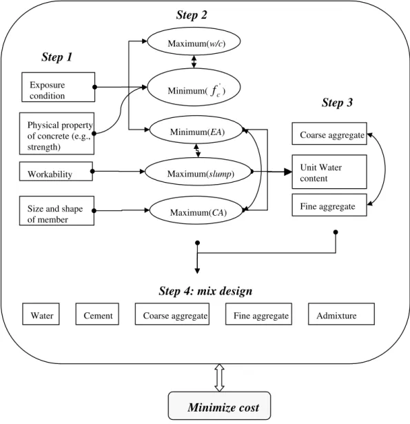
cement:sand:coarse aggregate) to the present-day mass and absolute-volume method (ACI 211.1-91 19211.1-91). A four-step mix design procedure is illustrated in Fig. 1. Step 1 entails specifying exposure condition, workability of freshly mixed concrete, and strength and durability
requirements of hardened concrete. Once this is specified, Step 2 follows code specified design procedures to satisfy minimum/maximum requirements, i.e. maximum water cement ratio (w/c
ratio), minimum 28 days specified strength ( ), minimum entrained air (EA), maximum slump,
and maximum coarse aggregate (CA). Step 3 entails computing the required unit water content, coarse aggregate and consequently the fine aggregate (FA). Finally, Step 4 specifies the final water, cement, coarse aggregate, fine aggregate and admixture content. Typically, the mix design is verified in the laboratory through trial mix, and adjustments are made accordingly. The final proportioning of the mix design has to be verified through concrete mix made in the field, since variation may arise due to different mixers, pumping properties and wall effect (Neville 1997). Moreover, the quality of the final in-place concrete is determined by the prevalent construction quality. Hence, from batching to concrete placement, stringent control has to be exercised as any deviation may compromise the structural integrity and durability of the structure. As shown in Fig. 1, there is an infinite possibility of obtaining the desired mix design specification, however, the desirable one is the one that satisfies the design constraints at minimal cost.
'
c f
The mix design involves a complex and nonlinear procedure that is influenced by the material interaction and culture of construction quality. Hence, it is difficult to develop a comprehensive analytical model by considering all design variables. Typically, concrete mix companies have extensive records of their past mix proportions, which can be used to develop a model for the design procedure. Automation of the mix proportioning can be carried out with different soft computing techniques. Soft computing is a conglomerate of computing techniques that include fuzzy-based methods, neuro-computing, genetic computing, probabilistic reasoning, genetic algorithms, chaotic systems, belief networks, and learning theory (Zadeh 1997). The soft computing techniques effectively explore the relationship among independent and dependent variables without any assumptions about the relationship (e.g., a linear relationship) between the various variables.
Various authors have used a standard multilayer feedforward artificial neural network (ANN) to predict the compressive strength of concrete (e.g. Lai and Serra 1997; Yeh 1998; Oh et al. 1999; Ni and Wang 2000; Hong-Guang and Ji-Zong 2000; Lee 2003; Kim et al. 2004; Chiang and Yang 2005) where a back propagation algorithm (BPNN) is used to train the network existing datasets. Kim et al. (2005) have further enhanced the previously reported (Kim et al. 2004) ANN using probabilistic neural network method to handle uncertainty and save computational time. Jain et al. (2005) forwarded further insight into the implementation and discussions on the efficiency of neural network models for concrete mix.
The main advantage of using ANN is their flexibility and ability to model nonlinear
relationships. However, the ANN models have often been criticized for acting as a “black box.” The knowledge contained in an ANN model is maintained in the form of a weight matrix that is
hard to interpret and can be misleading at times. In other words, the ANN models do not have the ability to incorporate additional knowledge or expertise into the model. Although qualitative modeling methods can be used to capture human knowledge, such models will naturally suffer from subjective human judgments. One way to overcome many of these shortcomings is to use fuzzy models or fuzzy inference systems (FIS) that can handle the uncertainties arising from insufficient knowledge, partial truth and vagueness (Zadeh 1973). These models combine the transparent linguistic representation of expert knowledge with the ability to learn from datasets. Various fuzzy modeling techniques have been presented in the literature (e.g., Sugeno and Yasukawa 1993, Klir and Yuan 1995, and Emami et al 1998). Jang (1993) proposed an adaptive network-based fuzzy inference system (ANFIS) to constructs a fuzzy inference system (FIS) in which membership functions is adapted using a back propagation algorithm in combination with the least-squares optimization.
ANFIS has recently been used in civil and environmental engineering applications. Akbuluta et al. (2004) used ANFIS for data generation of shear modulus and damping ratio in reinforced sands. Chau et al. (2005) used ANFIS and ANN for comparison of flood forecasting models and reported that ANFIS obtained optimal results. Chang and Chang (2005) utilized it to build a prediction model for reservoir management. Vernieuwe et al. (2005) applied it to the modeling of rainfall–discharge dynamics. Nayak et al. (2004) applied it to model hydrologic time series, and reported that ANFIS was superior to ANN and other statistical methods.
In this study, ANFIS is introduced as a tool to develop a fuzzy model that can estimate
compressive strength of concrete given its mix proportioning. Previously reported data (Kim et al. 2004, 2005) are used to train and validate the fuzzy model. The estimated strengths are
compared with the reported concrete strengths. The results highlight the utility of ANFIS in the construction industry. The outline of the paper is as follows. First, the concept of fuzzy based methods, including fuzzy inference systems and fuzzy modeling is explained briefly. Second, the implementation and derivation of an ANFIS based model is discussed. Third, ANFIS is used to develop a FIS model for estimation of concrete strength. The results are verified using actual concrete mix proportioning datasets reported in the literature, and the corresponding coefficient of determination r2 are computed. Finally, sensitivity analysis is carried out to highlight the impact of each mix constituents on the estimate concrete strength.
Fuzzy modeling methods
Fuzzy logic was initially used to formulate linguistic information (Zadeh 1965). Later its potential to model complex multi-input-multi-output systems, where classical mathematical methods failed, is realized. This is followed by the use of fuzzy inference system (FIS), also known as fuzzy rule-based systems or fuzzy models, in control and modeling problems in which there is usually some numerical information available, although incomplete and uncertain. A key feature of the FIS is that it can readily integrate expert knowledge in the form of linguistic information and uncertain numerical data in the form of input-output records into a model and then use it for approximate reasoning. According to Zadeh (1973), the FIS contains three features:
• linguistic variables instead of, or in addition to numerical variables; • relations between the variables in terms of IF-THEN rules; and
• an inference mechanism that uses approximate reasoning algorithms to formulate complex relationships.
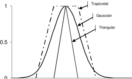
These features can be explained using the notion of fuzzy sets. A fuzzy set is a collection of ordered pairs that describe the relationship between an uncertain quantity and a membership function μ(x), where 0≤μ(x)≤1. A fuzzy number is a normal and convex fuzzy set in a continuous universe of discourse in which the variable is defined. Figure 2 shows the commonly used fuzzy numbers including triangular, trapezoidal, and Gaussian shape fuzzy numbers. Finally, a linguistic variable can be regarded as a variable whose value is a fuzzy number, but fuzzy numbers can also represent numerical variables without being firmly connected to
linguistic terms. An excellent introduction to the fuzzy set theory and fuzzy logic can be found in (Klir and Yuan, 1995; Lee, 1990a, b). In this section, the components of the FIS and the methods for constructing a FIS are explained.
Fuzzy inference system (FIS)
The information of the FIS is encapsulated in two modules: a fuzzy knowledge base and an inference mechanism. The former is a model developed based on expert knowledge and/or input-output data. The inference mechanism then uses the knowledge base to estimate the input-output of the system for given inputs. A modularized design of the FIS enables it to maintain a generic
processing structure that is capable of dealing with various systems in different application domains (e.g., physical, medical, financial) as long as a relevant knowledge base is defined. Also, the FIS can be readily updated by modifying the knowledge base using new information as it becomes available.
Knowledge base - The knowledge base defines the relationships between the input and output parameters of a system. The most commonly used representation of the input-output
relationships is Mamdani type fuzzy models (after Mamdani, 1977). In this type of fuzzy models, linguistic propositions are used both in antecedent and consequent parts of the IF-THEN rules.
Another type of representing the input-output relationships is Takagi-Sugeno-Kang (TSK) (Takagi and Sugeno 1985) fuzzy models in which the antecedent part of the rules is composed of linguistic propositions, but the consequent parts is defined by either a constant number (0th order)
or linear equations (1st order). A 1st-order TSK model of a multi-input-single-output system may
be represented by a set of linear subsystems (rules) each of which defined by a linear consequent statement,
i
R : IFx1isAi1AND …xmis Aim THEN yi =bi0+bi1x1+K+bimxm, i=1 K, ,n
(1)
where Ri represents the ith rule, n is the total number of rules, xj (j=1,K,m)are the input variables, is the output variable, is an input fuzzy set defined in the input space , and
are the consequent parameters. Thus, every rule is a local fuzzy relationship that maps a part of the multidimensional input space U into a certain part of the output space V .
i
y Aij Uj
ij b
It has been demonstrated (Sugeno and Tanaka 1991) that the TSK models can accurately represent complex behavior with a few rules. Although the TSK fuzzy models are
computationally less involved than the Mamdani type fuzzy models, the difficulty in defining a numerical function for the output propositions has often made them less attractive in fuzzy applications. This problem is resolved when the model is constructed automatically based on input-output data acquired from the systems. Another problem with the TSK models is that it is difficult to assign an appropriate linguistic term to the consequence propositions of the TSK models, but this will not be a problem if a qualitative model of the system is not required.
The rule base of a complex system usually requires a large number of rules to describe the behavior of a system for all possible values of the input variables. This is referred to as the “completeness” of a fuzzy model. The aggregation of the rules described in (1) forms a rule base that is valid over the entire application domain. The aggregation is obtained using the union of the rules or subsystems as,
Un i i R R 1 = =
= R1 ALSO R2 ALSO … ALSO Rn
(2)
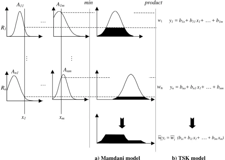
Inference mechanism – The inference mechanism of Mamdani type and TSK fuzzy models are slightly different. Mamdani’s inference mechanism (Fig. 3a) consists of three connectives: the aggregation of antecedents in each rule (AND connectives), implication (i.e., IF-THEN connectives), and aggregation of the rules (ALSO connectives). The operators performing the connectives distinguish the type of fuzzy inferencing. The AND and ALSO connectives are chosen from a family of t-norm and t-conorm operators, respectively. Comprehensive
discussions on t-norm (e.g., minimum and product operators) and t-conorm (e.g. maximum and sum operators) can be found in (Lee, 1990a, b). The implication (IF-THEN connective) also uses t-norm operators, but not necessarily identical to the ones used for the AND connectives.
The inference mechanism of TSK models (Fig. 3b) is more straightforward than the more common Mamdani’s type because the outputs of individual subsystems are crisp numbers. An algebraic product operator is usually selected to perform the t-norm to simplify the computations further. The result of implication of each rule is a weight factor that indicates the rule degree of firing (dof), . The aggregation of the rules is simply adding the weighted average of the output of the individual rules. Thus, the crisp output of a TSK model is given by,
i w
*
i n i n k k i y w w y
∑
∑
= = = 1 1 * (3) Fuzzy modelingThere are two basic approaches for developing a FIS: direct approach and system identification (Yager and Filev 1994b). In the direct approach, the information extracted from the expert knowledge is used to:
• specify the input, state, and output variables;
• determine the partitions of input and output variables in their universes of discourse, and optionally label the partitions with appropriate linguistic terms;
• define a set of IF-THEN statements (rules) that represent the relationships between the system variables;
• select an appropriate reasoning method; and finally, • evaluate the model adequacy.
Direct approach is essentially simple and intuitive, but it has inherent limitations. The main limitation is due to the fact that quantitative observations provide an overview of the
performance of the system, but do not explicitly determine the structure or parameters of the model. Also, it is often the case that an expert cannot tell linguistically what kind of outcome he expects or what kind of action he takes in a particular situation. As a result, the adequacy of the direct approach is restricted to the boundaries of the expert knowledge. In other words, if the expert knowledge about the system is incomplete and subjective, then so will be the model.
Another approach for developing a FIS is system identification. In this approach, the FIS is developed based on the input-output data (training data) obtained from the actual system. System identification is predominantly useful when a predetermined model structure based on
characteristics of variables is not available. Therefore, system identification can increase the objectivity of fuzzy modeling by introducing new knowledge to the model (Zadeh 1991). System identification is divided into two parts: structure identification and parameter identification (Sugeno and Yasukawa 1993). Similar to the direct approach, the objective of structure identification is to determine the input and output variables, partitions of the input and output spaces (i.e., fuzzy sets), relationships between the input and output variables (IF-THEN rules), and finally the number of rules. Parameter identification involves adjusting the parameters of the model obtained in the first part so that a performance index such as the root mean square of the output errors is minimized. The parameters of a TSK type fuzzy model define the input fuzzy sets Aij and the output coefficients bij of (1).
Structure identification - The input variables are selected from a pool of input candidates that most likely affect the output. Typically, there is no systematic way to specify the input
candidates, and hence selection is primarily carried out based on experience or common sense. Subsequently, given a finite number of input candidates and the training data, the input variables can be selected using the combinatorial algorithm described in (Tagaki and Sugeno 1985). In the latter, first a combination of input variables is selected from of a number of input candidates. Next, the optimum premise and consequent parameters are identified according to the input-output data and a performance index (e.g., mean square of differences between the model input-output and output data) is calculated. The optimal combination of input variables is the one that yields the minimum performance index.
The selection of the input variables is generally a complicated problem requiring iterative algorithms, if a priori knowledge of the system is not available. At this point, a general
understanding of the system performance or a sensitivity analysis of the input candidates prior to modeling can help reducing the number of input candidates.
The most important step of structure identification is the rule generation. Clustering of the input-output data is an intuitive approach to rule generation. The idea of clustering is to produce a concise representation of a system’s behavior by dividing the output data into a certain number of fuzzy partitions. The fuzzy C-Means (FCM) clustering algorithm (Bezdek 1981, Bezdek et al. 1987) has been widely studied and applied in many applications.
The convergence of the FCM optimization similar to most optimization problems depends on the choice of initial values (i.e., the number of clusters and initial cluster centers c νi). Yager and Filev (1994a) proposed a simple and effective clustering algorithm, called the mountain method, for estimating the number and initial location of cluster centers. In this method, a grid is
generated for data space of each input and output variable, and then a potential value for each grid point based on the distances to the actual data points is calculated. The grid points with high potential values correspond to the cluster centers. The problem with this clustering method is that the computational load increases exponentially with the number of input variables. Chiu (1994) proposed a modified form of the mountain method, called subtractive clustering, which significantly decreases the computational load, especially for systems with a large number of input variables. In this method, the potential value is calculated with respect to the actual data points not some inscribed grid points. The potential of a data point is given by,
1
i P
i
n i e P n j r x x i a j i , , 1 , 1 4 1 2 2 K = =
∑
= − − (4)where ra is a positive constant. The first cluster center is at ν1 that has the highest potential
value . Subsequently, the potential values of the remaining data points
are updated with respect to the first cluster by, n i Pi ), 1,K max( 1 0 = = π 1 , , 1 , , 2 , 2 2 1 4 1 1− = = − = − − − − − n i c k e P P b k i r x k k i k i K K ν π (5)
where is a positive constant and c is the total number of clusters. The procedure is repeated
until all cluster centers are obtained. The parameters and are used to adjust the distance between the clusters. Typically, the clusters stand in an appropriate distance when . In this paper, subtractive clustering is used to partition the input space and find the initial structure of the FIS. b r a r rb a b r r =1.5
The number of rules is an important parameter of the FIS. Clearly, the appropriate number of rules depends on the complexity of the system. According to Sugeno and Yasukawa (1993), the number of fuzzy rules corresponds to the order of a conventional model where an optimal model minimizes both the order and the output error. A statistical analysis for evaluating the optimal order of a model is discussed by Akaike (1974). A large number of rules, similar to a high order of a model, will bias the model towards specific data that can be imprecise or even erroneous. On the other hand, less number of rules will likely increase the output error, which is essentially equivalent to disregarding the effect of some of the data points containing valuable information.
Thus, the optimal number of rules can be obtained from a tradeoff between the number of rules and the output error.
n
The number of rules will be automatically determined through clustering the input and output spaces. Each cluster center is used as the basis of a rule that describes the system behavior. Thus, the neighborhood radii and can be selected such that an optimal number of rules is
achieved.
a
r rb
Parameter identification – Parameter identification concerns the adjustment of the antecedent and consequent membership functions. In general, parameter identification is more
straightforward than structure identification, especially when an initial structure of the model is determined based on expert knowledge or through clustering. In this paper, parameter
identification is carried out using Adaptive Network-based Fuzzy Inference System (ANFIS) (Jang 1993), which is also called Adaptive Neuro-fuzzy Inference System. The ANFIS algorithm basically provides a learning technique for extracting information from an input-output dataset viz., training data, and setting up the antecedent and consequent parameters of a fuzzy inference system, accordingly.
The ANFIS is essentially an adaptive multilayer feedforward network whose mathematical functionality is equivalent to a fuzzy inference system (FIS). The network is composed of a number of nodes connected through directed links. Each node is a processing unit that performs a node function on its incoming signal and yields the node output. The links only specify the direction of signal flow from one node to another. If a node function depends on certain
parameter values (i.e., node’s parameter set is nonempty), the node is an adaptive node. If a node function is fixed (i.e., node’s parameter set is empty) then it is a fixed node. The output of the
nodes as well as the overall behavior of the adaptive network can be modified by changing the node function parameters. Thus, these parameters can be updated according to the training data to achieve a desired input-output mapping.
The ANFIS network consists of the following five layers:
Layer 1: Every node i in this layer is an adaptive node with a node output O1,i given by
r j n i x O1,i =μAij( j), =1,K, =1,K, (6)
where is the input to the node, is a fuzzy set associated with the node, is the number of inputs, and is the number of rules. The use of Gaussian-shaped fuzzy sets is usually preferable from a computational point of view. A Gaussian fuzzy set with a maximum membership equal to 1 and minimum membership equal to 0 is given by,
j x Aij m n
(
)
⎪⎭ ⎪ ⎬ ⎫ ⎪⎩ ⎪ ⎨ ⎧ − − = 2 2 ij ij A a c x exp ij μ (7)where aijand cij are the antecedent parameters of the FIS.
Layer 2: Every node i in this layer is a fixed node, labeled Π , which multiplies the incoming signals and sends the product out.
∏
= = = m j j A i i w x O ij 1 , 2 μ ( ) (8)where is the degree of firing strength (dof) of rule . Any t-norm operator that performs AND connective can be used as the node function in this layer.
i
Layer 3: Every node in this layer is a fixed node labeled N. The ith node calculates the ration of
the ith rule’s firing strength to the sum of all rules’ firing strength.
∑
= = = n k k i i i w w w O 1 , 3 (9)where w is called the normalized dof of each rule. i
Layer 4: Every node i in this layer is an adaptive node with a node function
) ( 0 1 1 , 4i wiyi wi bi bi x bimxm O = = + +K+ (10)
where w is the output of layer 3, and i bij, j =1,K,mare the consequent parameters of the FIS.
Layer 5: The single node in this layer is a fixed node labeled Σ that composes the overall output as the summation of all incoming signals, i.e.,
∑
∑
∑
= = = = = n i i i n i i i n i i w y w y w O 1 1 1 1 , 5 (11)The above 5-layer network is functionally equivalent to a TSK type fuzzy inference system.
The parameter identification of the TSK models involves the determination of antecedent
parameters and and consequent parameters using a given input-output dataset. A basic approach for identifying the parameters of an adaptive network is based on gradient method (Werbos 1974). The learning rule concerns how to recursively obtain a gradient vector in which
ij
each element is defined as the derivative of an error measure with respect to a parameter. In gradient method, the learning rule is a chain rule, generally referred to as “back propagation” (Rumelhart et al. 1986) because the gradient vector is calculated in the direction opposite to the flow of the output of each node.
Although the gradient method seems a straightforward approach for the determination of the parameters of an adaptive network, this method is generally slow and likely to become unstable or trapped in local minima. The ANFIS constructs a fuzzy inference system (FIS) using a hybrid of the least squares estimate (LSE) and gradient descent proposed by Jang (1993) (see also Jang and Sun 1995). Specifically, the learning procedure uses the least squares estimate in a forward pass and gradient descent in a backward pass. In the forward pass, the network is simulated till layer 4 and the consequent parameters are identified by the least squares estimate under the condition that the antecedent parameters are fixed. In the backward pass, the error rates propagate backward and the antecedent parameters are updated by the gradient descent. The learning process is continued based on a learning rule, usually represented by the discrepancy between the desired output and the network output under the same input conditions. This discrepancy is called the error measure, which is usually defined as the sum of the squared differences between the desired and network outputs.
ANFIS model development for concrete strength estimation
The efficiency of the proposed ANFIS modeling technique is illustrated using the mix proportioning and material characterization data reported in Kim et al. (2004) and Kim et al. (2005). A three step procedure on the implementation of ANFIS to estimate concrete strength
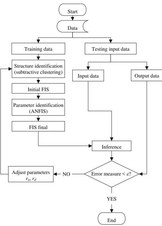
using mix design is illustrated in this section. Fig. 4 shows the flowchart of the proposed modeling approach.
Step 1: Preparation of training data
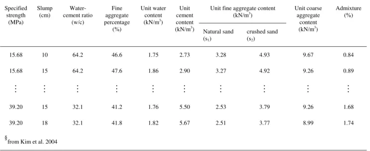
The concrete mix constituents used in the model development are similar to those used in Kim et al. (2004) and Kim et al. (2005). The reported data were gathered from actual mix proportions of two companies, Company A and Company B. The overall basic material properties between the two companies are similar, with the exception of sand used. Company B uses only natural sand whereas Company A mixes both natural and crushed sand. Sample input data of the specified concrete mix proportions of Company A and B are presented in Tables 1a and 1b, respectively. Further, the main difference between the reported Kim et al. (2004) and Kim et al. (2005) data is the units assigned to the mix proportions. Kim et al. (2004) use kN/m3 for water, cement, fine
aggregate and coarse aggregate contents, whereas Kim et al. (2005) use kg/m3 for those
proportions Consequently, to combine the two datasets, the kN/m3 units (shown in Tables 1a and
1b) are converted into kg/m3.
The Company A and B data were combined for model training under the assumption that the data are commensurate. Hence, the final training data for Company A and B consist of 45 data points each. Further, a combined model of Company A and B, henceforth described as Company A-B is generated using a total of 90 training data points. It is noted that Company A and B have different fine aggregate constituents. Thus, for combined Company A-B data, the natural and crushed sand of Company A are combined and represented with a single fine aggregate (FA) label. For brevity, data are not repeated here; curious readers are referred to Kim et al. (2004) and Kim et al. (2005).
Kim et al. (2004) and Kim et al. (2005) have considered nine different concrete mix
proportioning parameters to model the 28-day compressive strength. The efficiency of a given model can be demonstrated using minimal input parameters to capture the desired model output. Hence, in this paper, initial screening is carried out to eliminate any redundant input parameter. For example, the simultaneous use of water-cement ratio and the corresponding water and cement contents as input parameters is redundant. Hence, the input parameters are divided into two groups, absolute variables and relative variables (Table 2). The absolute value modeling includes absolute values, input parameters entail, where possible, parameters without any relative ratios, e.g. using only unit water content and unit cement content, without the w/c ratio, specified concrete strength, slump, etc. The input of the relative value modeling includes relative ratios where possible (e.g., w/c ratio, fine aggregate percentage, etc…).
Step 2: Structure and parameter identification
ANFIS is used for structure and parameter identification as outlined in the previous section. The models are generated using datasets of Company A, Company B and the combination of
Company A and B that are referred to as Model A, Model B and Model A-B, respectively. Moreover, each of the three models is implemented for absolute variables and relative variables, which are referred to as absolute model and relative model, respectively. In this way, a total of six models are generated. Initial sensitivity analysis is carried out to observe if there is any significant difference between the actual concrete strength and those predicted using the six models. The analysis showed that the results are only slightly different. Nevertheless, for a pragmatic model application, where a more generic model with the minimum number of inputs is
typically more desirable, Model A-B is preferable. The ensuing discussion is only for the relative Model A-B, but the derived conclusion is equally applicable to the other five models.
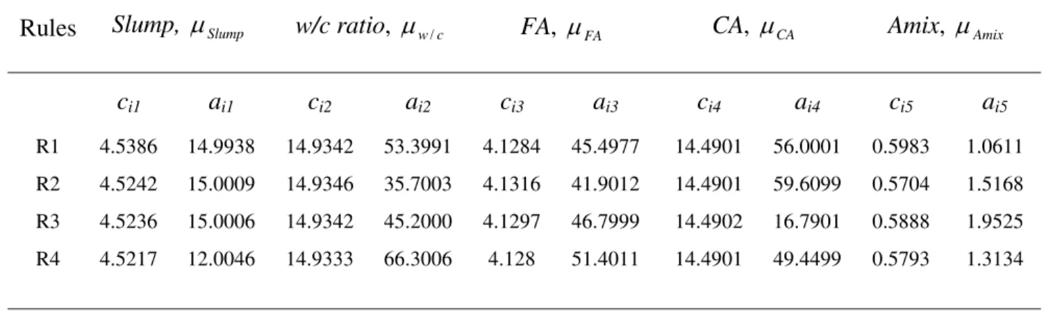
The FIS generated for the five relative input parameters (Table 2: slump, w/c ratio, FA, CA, Amix) has four rules. Each input parameter is modeled using a Gaussian type membership function (7). Result of coefficients of the Gaussian type membership function, for slump (μSlump), w/c ratio (μw /c), FA (μFA), CA (μCA), and Amix (μAmix) are summarized in Table 3. For example, from Table 3, the μSlump associated with Rule 1 is:
( ) ⎟ ⎠ ⎞ ⎜ ⎝ ⎛ − − = 14.9938 2 5386 . 4 2 1 ) ( x e x Slump μ .
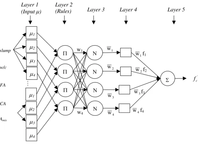
The ANFIS equivalent of the TSK model is illustrated in Fig. 5. As discussed in the previous section, the ANFIS is represented in five layers. Layer 1 corresponds to the membership functions (Table 3). Layer 2, is a product layer, which illustrate the firing strength of a rule. Hence, the ith rule firing strength (wi) of input parameters associated with Rule i is (8):
) ( ) ( ) ( ) / ( ) ( w/c FA CA Amix mix Slump i Slump w c FA CA A w =μ ×μ ×μ ×μ ×μ .
Layer three entails normalization of the ith rule strength to the sum of all rules firing strength (9):
4 3 3 1 w w w w w w i i = + + + .
Hence, w is called normalized firing strengths. Layer four computes the corresponding output i strength estimation of Rule i (10):
i O
(
b1 slump b2 w/c b3 FA b4 CA b5 A b0)
w y w
Oi = i i = i × + × + × + × + × mix + .
The parameters, {b1, b2, b3, and b4} are referred as consequent parameters (Table 4). For
example, the model output from Rule 1 can be shown as
(
0.0471 0.4684 / 0.4255 % 0.000988 8.866 34.46)
1
1 =w − ×slump− ×w c+ ×FA + ×CA− ×Amix+
O
.
Finally, the estimated concrete strength, , is obtained by summing the model output of the four rules (11): ' c f
∑
∑
∑
= = i i i i i i i i c w f w f w f'Step 3: ANFIS Model Validation
Model validation must be carried out using the input-output data that are not used for training to evaluate the efficiency the FIS in predicting concrete strength. The reported (Kim et al. 2004 and Kim et al. 2005) testing data points are combined in the model validation, which resulted in total of 24 data points for each of Model A and B, and 48 data points for Model A-B. The FIS model predicted and actual concrete strength are used for model validation. The results are plotted in Figs. 6a to 6e. Figures 6a, 6c, and 6e show result of the absolute model validation of Model A, B, and A-B, respectively. Similarly, Figs. 6b, 6d, and 6f show result of the relative model validation of Model A, B, and A-B, respectively. A linear regression fit is performed between the actual and predicted concrete strength. The corresponding absolute and relative model coefficient of determination r2 values are as follows: Model A (0.999, 0.984), Model B (0.970, 0.995) and Model A-B (0.999, 0.998).
Discussion
Concrete mix proportioning is a highly nonlinear process that is also subject to experimental error (Kim et al. 2004). Reliable prediction of concrete strength necessitates the development of models which are tolerant of various manifestations of uncertainty. Identification of dominant parameters can help to implement stringent monitoring and quality control during mix
proportioning (Jain et al. 2005). A sensitivity analysis is commonly carried out using random sampling (Monte Carlo-type simulations) where the probability distributions for input data can either be assumed or derived from observations. Thereafter, the rank correlation method (Cullen and Frey 1999) is applied to the results of the Monte Carlo simulations to identify input
data/parameters that dominate the output. The rank correlation method involves the determination of coefficient of determinations, which measure the strength of the linear relationship between two variables. The procedure utilized for the sensitivity analysis is as reported in Tesfamariam et al. (2005) and the basic steps are outlined here. For ns number of
realization,
For i = 1 to ns,
▪ Generate a uniformly distributed random numbers for the five input parameters (ranging between the min and max values),
▪ Compute the corresponding membership function (6) and (7), j x ) ( j Aij x μ
▪ Compute the dof (8) and normalized dof (9)
Next i
▪ For the n input-output results, rank order the results and perform rank correlation ▪ Normalize the rank correlation results and show the result on a tornado graph
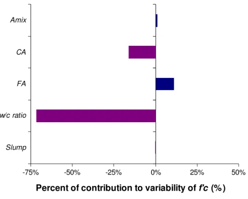
Sensitivity analysis of the FIS model is carried out for 3000 realizations from the relative Model A-B, and the results of the rank correlation are normalized to the sum of one and are plotted in a tornado graph (Fig. 7). Figure 7 shows that an increase in CA (16% contribution) and w/c ratio (72% contribution) decreases the concrete strength. Clearly, the contribution of Slump is not considerable. On other hand, an increase in FA (11% contribution) and Amix (1% contribution), albeit to a smaller degree, is followed by an increase in the concrete strength. It is interesting to note that impact of CA, w/c ratio, Amix and FA is in agreement with the results reported in Neville 1997. Overall the w/c ratio is the most dominant parameter towards the variability of the concrete strength. This reinforces our intuitive understanding that stringent quality control of the in situ w/c ratio should be implemented.
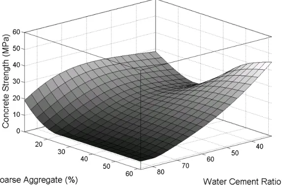
Further, two parameters at a time simulation is carried out for the three most dominant variables; w/c ratio, CA and FA. Figure 8a shows the simulation between w/c ratio and CA. At a higher CA content, e.g., 60%, there is a linear decrease in concrete strength with an increase in w/c ratio. At a lower CA content, e.g. 10%, the variation of w/c ratio from 40% to roughly 65% show
negligible variation. However, at CA = 10%, significant decrease in concrete strength is observed with increase in the w/c ratio from 65% to 80%. At a lower w/c ratio, e.g. <50%, an increase in CA content (from 10% to 30%) is followed by a decrease in concrete strength. However, with further increase in CA content (from 30% to 60%), the concrete strength
underlined that the reason for this effect is not clear. At a higher w/c ratio, an increase in CA content (beyond 35%) reaches minima and the variation is not significant.
Figure 8b shows the relationship between FA and w/c ratio. In general, an increase in FA and a decrease in w/c ratio are followed by a linear increase in concrete strength. Figure 8c shows the variation of CA and FA in the estimated concrete strength. At any level of the FA content, increase in CA is followed by a decrease in concrete strength; however, after 35% CA content, it reaches minima. Similarly, and increase in FA is followed by an increase in concrete in strength, however, after 48% FA, it reaches a maxima.
The accuracy of the ANFIS model generated from the input parameters may be compromised outside the range of the training datasets. The inputs parameters for the proposed ANFIS model discussed in the paper are bounded within the following ranges: Slump, mm [5, 18]; unit water content [160, 185]; unit cement content, kg/m3 [228, 524]; unit fine aggregate content, kg/m3
(663, 1004); unit coarse aggregate content, kg/m3 [882, 1060]; admixture, % [0.7, 2.6]; specified
strength, MPa [10.8, 39.2]. Extrapolating the model outside these limits should be carried out with caution.
Conclusions
Concrete mix proportioning is a nonlinear process, for which developing a comprehensive and reliable analytical model is rather challenging, if not impossible. Typically, concrete
manufacturing companies have extensive datasets of past mix proportions, which can be used for modeling and validation. Hence, the concrete industry can benefit from their historical datasets in conjunctions with soft computing techniques to automate mix proportioning and predict the
strength of the final product, reliably. This study presents ANFIS modeling for concrete strength estimation from concrete mix proportioning. The open architecture of the ANFIS model is appealing as it captures the designer’s intuitive experience as well as the numerical information included in the datasets. The ANFIS modeling also allows post-modeling adjustment and fine tuning based on the new datasets as they become available. The ANFIS modeling has a
significant potential in the concrete industry. Sensitivity analysis is carried out to identify critical parameters that impact the concrete strength. Results of this analysis can be used to develop in situ construction quality. The ANFIS model is developed for absolute input parameters where necessary (e.g. unit water content (kg/m3), unit FA content (kg/m3), etc…). However, to
minimize the number of input parameters, relative input parameters (e.g. w/c ratio (%), FA percentage (%), etc…) are taken into account where possible. The proposed model is tested and validated with actual reported data in the literature. The coefficients of determination r2 of the corresponding absolute and relative models are as follows: Model A (0.999, 0.984), Model B (0.970, 0.995) and Model A-B (0.999, 0.998).
The proposed ANFIS modeling method is a step forward toward the development of a
comprehensive model for the concrete industry. In any future development, the concrete strength modeling should incorporate external factors that impact the concrete strength, such as
construction quality, environmental condition, etc. Further, this modeling approach can be used at different stages of the concrete industry. These stages include, but not limited to, mix design proportioning, simulation of concrete strength using mix design proportioning, estimation of in situ concrete strength given the history of construction quality and in situ construction quality monitoring using the a measured slump and air content. Finally, the use of soft computing
techniques such as ANFIS modeling allows the concrete industry avoid the risk of faulty or deficient concrete that often entails durability and safety problems.
References
ACI 211.1-91. (R2001). “Standard practice for selecting proportions for normal, heavyweight and mass concrete.” ACI Committee 211 Report, American Concrete Institute, Detroit.
Akaike, H. (1974). “New look at the statistical model identification.” IEEE Transactions on Automatic Control, 19, 716-723.
Akbuluta, S., Hasiloglub, A.S. and Pamukcuc, S. (2004). “Data generation for shear modulus and damping ratio in reinforced sands using adaptive neuro-fuzzy inference system.” Soil Dynamics and Earthquake Engineering, 24, 805–814.
Bezdek, J.C. (1981). Pattern Recognition with Fuzzy Objective Function Algorithms, Plenum Press, New York.
Bezdek, J.C., Hathaway, R., Sabin, M., and Tucker. W. (1987). “Convergence theory for fuzzy c-means: Counterexamples and repairs.” The Analysis of Fuzzy Information, Bezdek J. (ed), CRC Press, 3, Chap. 8.
Chang, F.-J. and Chang, Y.-T. (2005). “Adaptive neuro-fuzzy inference system for prediction of water level in reservoir. Advances in Water Resources.” Advances in Water Resources, in press.
Chau, K.W., Wu C.L. and Li Y. S. (2005). “Comparison of Several Flood Forecasting Models in Yangtze River.” Journal of Hydrologic Engineering, 10(6), 485-491.
Chiang, C.-H. and Yang, C.-C. (2005). “Artificial neural networks in prediction of concrete strength reduction due to high temperature.” ACI Materials Journal, 102(2), 93–102.
Chiu, S.L. (1994). “Fuzzy model identification based on cluster estimation.” Journal of Intelligent and Fuzzy Systems, 2, 267-278.
Cullen, A.C. and Frey, H.C. (1999). Probabilistic Techniques in Exposure Assessment: a Handbook—for Dealing with Variability and Uncertainty in Models and Inputs. Plenum Press, New York, pp. 352.
Emami, M. R., Turksen, I. B., and Goldenberg, A. A., (1998). “Development of a systematic methodology of fuzzy logic modeling.” IEEE Transactions on Fuzzy Systems, 6(3), 346-361.
Hong-Guang, N., and Ji-Zong, W. (2000). “Prediction of compressive strength of concrete by neural networks.” Cement and Concrete Research, 30, 1245–1250.
Jain, A., Misra, S., and Jha, S.K. (2005). “Discussion of “Application of neural networks for estimation of concrete strength.”” Journal of Materials in Civil Engineering, 17(6), 736–738.
Jang, J. S. R. (1993). “ANFIS: Adaptive-Network-Based Fuzzy Inference System.” Transactions on Systems, Man, and Cybernetics, 23(3), 665-685.
Jang, J. S. R., and Sun, C. T. (1995). “Neuro-fuzzy modeling and control.” Proceedings of the IEEE, 83(3), 378-406.
Kim, D. K., Lee, J.J.; Lee, J.H.; and Chang, S.K. (2005). “Application of probabilistic neural networks for prediction of concrete strength.” Journal of Materials in Civil Engineering, 17(3), 353–362.
Kim, J. I., Kim, D. K., Feng, M. Q., and Yazdani, F. (2004). “Application of neural networks for estimation of concrete strength.” Journal of Materials in Civil Engineering, 16(30), 257–264.
Klir, G. J., and Yuan, B. (1995). Fuzzy sets and fuzzy logic – theory and applications, Prentice-Hall Inc., Englewood Cliffs, New Jersey.
Lai, S., and Serra, M. (1997). “Concrete strength prediction by means of neural network.” Construction and Building Materials, 11(2), 93–98.
Lee, C. C. (1990a). “Fuzzy logic in control systems: Fuzzy logic controller-Part I.” IEEE Transactions on Systems, Man, and Cybernetics, 20(2), 404-418.
Lee, C. C. (1990b). “Fuzzy logic in control systems: Fuzzy logic controller-Part II.” IEEE Transactions on Systems, Man, and Cybernetics, 20(2), 419-435.
Lee, S.C. (2003). “Prediction of concrete strength using artificial neural network.” Engineering Structures, 25, 849-857.
Mamdani, E. H. (1977). “Application of fuzzy logic to approximate reasoning using linguistic synthesis.” IEEE Transactions on Computers, 26(12), 1182-1191.
Nayak, P.C., Sudheer, K.P., Rangan, D.M., and Ramasastri, K.S. (2004). “A neuro-fuzzy
computing technique for modeling hydrological time series.” Journal of Hydrology, 291, 52– 66.
Neville, A.M. (1997). Properties of Concrete, 4th Ed., Wiley, New York.
Ni, H.G., and Wang, J.Z. (2000). “Prediction of compressive strength of concrete by artificial neural networks.” Cement and Concrete Research, 30, 1245–1250.
Oh, J. W., Lee, I. W., Kim, J. T., and Lee, G. W. (1999). “Application of neural networks for proportioning of concrete mixes.” ACI Materials Journal, 96(1), 61–67.
Rumelhart D. E., Hinton, G. E., and Williams, R. J. (1986). “Learning internal representations by error propagation.” Parallel Distributed Processing: Explorations in the Microstructure of Cognition, D.E. Rumelhart and J.L. McClelland, Eds., MIT Press, Cambridge, MA, 1, 318-362.
Sugeno, T. and Tanaka, K. (1991). “Successive identification of systems and its application to modeling and control.” Fuzzy Sets and Systems, 42(3), 315-334.
Sugeno, M. and Yasukawa, T. (1993). “A Fuzzy-Logic-Based Approach to Qualitative Modeling.” IEEE Transactions on Fuzzy Systems, 1(1), 7-31.
Takagi, T. and Sugeno, M. (1985). “Fuzzy identification of systems and its applications to modeling and control.” IEEE Transactions on Systems, Man, and Cybernetics, 15(1), 116– 131.
Tesfamariam, S., Rajani, B. and Sadiq, R. 2006. Consideration of uncertainties to estimate structural capacity of ageing cast iron water mains - a possibilistic approach. Canadian Journal of Civil Engineering, 33(8): 1050-1064.
Vernieuwe, H., Georgieva, O., Baets, B.D., Pauwels, V.R.N., Verhoest, N.E.C. and F.P. D. Troch (2005). “Comparison of data-driven Takagi–Sugeno models of rainfall–discharge dynamics.” Journal of Hydrology, 302, 173–186.
Werbose, P. (1974). Beyond regression: New tools for prediction and analysis in the behavioral sciences. PhD dissertation, Harvard University, Cambridge, MA.
Yager, R.R. and Filev, D.P. (1994a). “Generation of fuzzy rules by mountain clustering.” Journal of Intelligent and Fuzzy Systems, 2, 209-219.
Yager, R. R., and Filev, D. P. (1994b). Essentials of fuzzy modeling and control, Wiley, New York.
Yeh, I.-C. (1998). “Modeling of strength of high-performance concrete using artificial neural networks.” Cement and Concrete Research, 28(12), 1797–1808.
Zadeh, L.A. (1965). “Fuzzy sets.” Information and Control, 8, 338-353.
Zadeh, L.A. (1973). “Outline of a new approach to the analysis of complex systems and decision processes.” IEEE Transactions on Systems, Man, and Cybernetics, 3, 28-44.
Zadeh, L.A. (1991). “From circuit theory to system theory.” Facets of Systems Science (G.J. Klir Eds.), Plenum Press, New York.
Zadeh, L.A. (1997). “The role of fuzzy logic and soft computing in the conception, design and deployment of intelligent systems.” Software Agents and Soft Computing, Springer, New York.
LIST OF NOTATION
ij
A Input fuzzy set
ANFIS Adaptive Network-based Fuzzy Inference System
ij
a , cij Parameters of Gaussian-shaped function
ij
b Consequent parameters
c Subtractive cluster, total number of clusters
CA Coarse aggregate
dof Degree of firing strength
j
i, Counters
ε Error measure
FA Fine aggregate
FIS Fuzzy inference system
'
c
f minimum 28 days specified strength
n Total number of rules
i
O1, Node output of the ANFIS network
1
i
P Subtractive cluster, potential value
i
R ith rule
a
r , rb Subtractive cluster, adjustment parameters
TSK Takagi-Sugeno-Kang j
U Input space
V Output universe of discourse
i
ν Subtractive cluster, cluster centers
i
w Degree of firing strength
i
w Normalized dof of each rule
w/c ratio water cement ratio
j
x Input variables (j=1,K,m)
i
*
y Defuzzified crisp value
) x (
μ Membership function
0
π Highest potential value
List of Figures
Figure 1. Concrete mix proportioning
Figure 2. Typical Fuzzy Membership Functions
Figure 3. Fuzzy reasoning models
Figure 4. Flowchart of ANFIS model development for concrete strength modeling
Figure 5. ANFIS equivalent of TSK model for concrete strength modeling
Figure 6. Comparison of target and predicted concrete strength for a combined and relative model.
Figure 7. Sensitivity analysis of concrete strength input parameters using a tornado graphs
Figure 8a. Impact of variation in water cement ratio and coarse aggregate on the estimated concrete strength: Slump (10 mm), Amix (1.5%) and FA (50%)
Figure 8b. Impact of variation fine aggregate and water cement ratio on the estimated concrete strength: Slump (10 mm), Coarse Aggregate (40%) and Admixture (1.5%)
Figure 8c. Impact of variation in coarse aggregate and fine aggregate on the estimated concrete strength: Slump (10 mm), Water cement ratio (60%) and Admixture (1.5%)
Unit fine aggregate content (kN/m3) Specified strength (MPa) Slump (cm) Water-cement ratio (w/c) Fine aggregate percentage (%) Unit water content (kN/m3) Unit cement content (kN/m3) Natural sand (s1) crushed sand (s2) Unit coarse aggregate content (kN/m3) Admixture (%) 15.68 10 64.2 46.6 1.75 2.73 3.28 4.93 9.67 0.84 15.68 15 64.2 47.6 1.86 2.90 3.27 4.92 9.26 0.89 M M M M M M M M M M 39.20 15 32.1 41.2 1.76 5.50 2.53 3.79 9.26 1.68 39.20 18 32.1 41.8 1.82 5.67 2.51 3.77 8.99 1.74 §
from Kim et al. 2004
Table 1b. Sample Input Data, Specified Concrete Mix Proportions of Company B for Training§
Unit fine aggregate content (kN/m3) Specified strength (MPa) Slump (cm) Water-cement ratio (w/c) Fine aggregate percentage (%) Unit water content (kN/m3) Unit cement content (kN/m3) Natural sand (s1) crushed sand (s2) Unit coarse aggregate content (kN/m3) Admixture (%) 15.68 10 63.1 50.9 1.68 2.66 9.23 - 9.08 1.36 15.68 15 63.2 50.4 1.76 2.79 8.98 - 9.01 1.43 M M M M M M M M M 39.20 15 33.2 44.4 1.71 5.14 7.11 - 9.08 2.62 39.20 18 33.2 44.1 1.75 5.28 6.96 - 9.00 2.70 §
Table 2. Datasets of Specified Concrete Mix Proportions
Absolute value modeling Relative value modeling
Specified concrete strength (MPa) Slump (cm)
Unit water content (kg/m3)
Unit cement content (kg/m3)
Unit fine aggregate content (kg/m3)
Natural sand (s1), crushed sand (s2)
Unit coarse aggregate content (kg/m3)
Admixture (%)
Specified concrete strength (MPa) Slump (cm)
Water-cement ratio (w/c) Fine aggregate percentage (%) Coarse aggregate percentage (%) Admixture (%)
Table 3. Membership function of the Model A-B input parameters
Rules Slump, μSlump w/c ratio, μw /c FA, μ FA CA, μCA Amix, μAmix
ci1 ai1 ci2 ai2 ci3 ai3 ci4 ai4 ci5 ai5
R1 4.5386 14.9938 14.9342 53.3991 4.1284 45.4977 14.4901 56.0001 0.5983 1.0611 R2 4.5242 15.0009 14.9346 35.7003 4.1316 41.9012 14.4901 59.6099 0.5704 1.5168 R3 4.5236 15.0006 14.9342 45.2000 4.1297 46.7999 14.4902 16.7901 0.5888 1.9525 R4 4.5217 12.0046 14.9333 66.3006 4.128 51.4011 14.4901 49.4499 0.5793 1.3134
Table 4. Datasets of Specified Concrete Mix Proportions
Rules b1 b2 b3 b4 b5 b0
R1 -0.0471 -0.4684 0.4255 0.000988 -8.866 34.46
R2 -0.4072 0.2037 1.329 -0.9398 18.57 -59.22
R3 -0.06809 -1.013 1.298 1.09 3.304 -51.54
Exposure condition
Size and shape of member Step 1 Step 2 Workability Fine aggregate Coarse aggregate Unit Water content Step 3 Maximum(CA) Minimum(EA) Minimum( fc') Maximum(w/c)
Water Cement Coarse aggregate Fine aggregate Admixture
Step 4: mix design
Minimize cost Physical property
of concrete (e.g., strength)
Maximum(slump)
0 0.5
1 Trapizodal
Gaussian Triangular
K A11 A1m M M K x1 xm An1 Anm w1 R1 Rn wn i wyi =wi (bio+ bi1 x1+ K+ bim xm) min product a) Mamdani model y1 = b1o+ b11 x1+ K+ b1m yn = bno+ bn1 x1+ K+ bnm b) TSK model
Training data Testing input data Data Start Structure identification (subtractive clustering) Parameter identification (ANFIS) Initial FIS FIS final Inference Adjust parameters ra, rd NO End YES Output data Input data Error measure < ε?
slump Amix Π Π Ν Ν Σ Layer 1 (Input μ) Layer 2
(Rules) Layer 3 Layer 4 Layer 5
w1 w1 2 w 1 w f1 2 w f2 ' c f Π Π Ν Ν w4 3 w 4 w M μ1 μ2 μ3 μ4 3 w f3 4 w f4 w/c FA CA μ1 μ2 μ3 μ4
0 10 20 30 40 50 0 10 20 30 40 50
Target concrete strength (MPa)
P re di c te d c o nc re te s tr e ng th ( M P a ) r2=0.995 0 10 20 30 40 50 0 10 20 30 40 50
Target concrete strength (MPa)
P re di c te d c o nc re te s tr e ng th ( M P a ) r2=0.970 0 10 20 30 40 50 0 10 20 30 40 50
Target concrete strength (MPa)
P re d ic te d c o n c re te s tr e n g th (MPa ) r2=0.984 0 10 20 30 40 50 0 10 20 30 40 50
Target concrete strength (MPa)
P re d ic te d c o n c re te s tr e n g th (MPa ) r2=0.999 0 10 20 30 40 50 0 10 20 30 40 50
Target concrete strength (MPa)
Pr e d ic te d c o n c re te s tr e n g th (MPa ) r2=0.999 0 10 20 30 40 50 0 10 20 30 40 50
Target concrete strength (MPa)
Pr e d ic te d c o n c re te s tr e n g th (MPa ) r2=0.998 a) Model A: absolute c) Model B: absolute d) Model B: relative e) Model A-B: absolute f) Model A-B: relative b) Model A: relative
Figure 6. Comparison of target and predicted concrete strength for a combined and relative model.
-75% -50% -25% 0% 25% 50%
Percent of contribution to variability of f'c (% )
Slump w/c ratio FA CA Amix
Figure 8a. Impact of variation in water cement ratio and coarse aggregate on the estimated concrete strength: Slump (10 mm), Amix (1.5%) and FA (50%)
Figure 8b. Impact of variation fine aggregate and water cement ratio on the estimated concrete strength: Slump (10 mm), Coarse Aggregate (40%) and Admixture (1.5%)
Figure 8c. Impact of variation in coarse aggregate and fine aggregate on the estimated concrete strength: Slump (10 mm), Water cement ratio (60%) and Admixture (1.5%)