Publisher’s version / Version de l'éditeur:
Membrane Technology and Environmental Applications, pp. 75-95, 2012-12-31
READ THESE TERMS AND CONDITIONS CAREFULLY BEFORE USING THIS WEBSITE. https://nrc-publications.canada.ca/eng/copyright
Questions? Contact the NRC Publications Archive team at
[email protected]. If you wish to email the authors directly, please see the first page of the publication for their contact information.
NRC Publications Archive
Archives des publications du CNRC
For the publisher’s version, please access the DOI link below./ Pour consulter la version de l’éditeur, utilisez le lien DOI ci-dessous.
https://doi.org/10.1061/9780784412275.ch03
Access and use of this website and the material on it are subject to the Terms and Conditions set forth at
Fundamentals of membrane processes
Kumar, Ashwani
https://publications-cnrc.canada.ca/fra/droits
L’accès à ce site Web et l’utilisation de son contenu sont assujettis aux conditions présentées dans le site
LISEZ CES CONDITIONS ATTENTIVEMENT AVANT D’UTILISER CE SITE WEB.
NRC Publications Record / Notice d'Archives des publications de CNRC:
https://nrc-publications.canada.ca/eng/view/object/?id=a080b729-a245-4035-8369-c4af0ff9c512 https://publications-cnrc.canada.ca/fra/voir/objet/?id=a080b729-a245-4035-8369-c4af0ff9c512
CHAPTER 3
Fundamentals of Membrane Processes
Ashwani Kumar
3.1
Introduction
In order to develop energy efficient and economically viable membrane-based processes, one needs to understand the factors responsible for membrane performance and the means to determine the characteristics of the membranes and modules. This understanding is required at several different levels such as membrane materials, membrane formation, membrane pore size distribution, interaction of membrane material and feed components. Assembly of membranes into modules including determination of their fluid flow behaviour and tolerance to the operating conditions is essential. Finally membrane deployment in combination with other unit operations utilized in the process chain needs to be discussed. Accordingly, this chapter is divided into three major sections dealing with various aspects of membranes. In Section 3.2, membrane materials and their properties for different types of applications are presented. In Section 3.3, different models of fluid flow through the membranes including thermodynamic and phenomenological models are discussed. In Section 3.4, application of Computational Fluid Dynamic (CFD) studies of overall feed/permeate flow in modules and its impact on process development is presented.
3.2
Membrane Materials and Properties
Membranes are made from a variety of materials including polymeric, ceramic, and metallic as well as a combination of more than one material such as ceramic coated metallic membranes. Selection of these materials in large part depends on performance requirements dictated by the feed properties and separation goals. For example, if the feed contains significantly high amounts of aggressive solvents and has to be processed at higher than 140 0C, a polymer-based membrane would not be suitable for processing
this feed. On the other hand, if the feed has a pH of 2–11 and a target compound to be separated is a lower molecular weight dissolved component, then a polymeric membrane
might be a more suitable choice. In addition to the membrane material characteristics, morphology of membrane relating to its structure during formation also plays an important role. An asymmetric membrane with a thin separating layer supported by the porous structure will be less fouling prone than a homogenous membrane. Furthermore the hydrophobic/hydrophilic nature of the membrane material will also have an impact on the permeation characteristics. It is very important to realize that selection of the type of membrane is determined on the basis of its separation performance and its compatibility with the feed. Membrane materials, their formation and performance for various processes are well described in membrane text books (Ho and Sirkar, 1992; Matsuura, 1993; Cheryan, 1998).
The literature on the usage of different types of materials for making membranes for laboratory scale use is very extensive; a comprehensive review is beyond the scope of this section. The most widely used materials for different membrane processes are listed in Table 3.1.
Table 3.1 Widely used membrane materials for different membrane processes. Membrane Process Membrane Materials
Gas and vapour
permeation; Cellulose acetates, Polyetherimide,polysulfone, polydimethylsiloxanes, Poly vinyl alcohol, polydimethylsiloxanes Reverse Osmosis Cellulose acetates, polyamides, polyimides and various thin film
composites of other polymeric materials on polysulfones Nanofiltration Polyacronitrile, polyvinyl alcohol, silicone
Ultrafiltration Polyacronitrile, polyvinyl alcohol, polyvinyledene fluoride, regenerated cellulose, ceramic materials,
Microfiltration Polycarbonates, cellulose nitrate, carbon composites, stainless steel coated with ceramic, modified polyethylene and
polypropylene
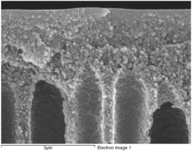
Membranes are formed using different techniques such as gelation, thermally induced phase separation, slip casting and track etching and coating substrates with or without reactions. In addition to membrane materials, the properties of the membranes also depend on the morphological structure. In a microfiltration (MF) membrane formed by bombarding nuclear particles on polycarbonate film, the pore sizes and surface porosity will play a major role as the film porosity is not important. On the other hand, bulk porosity of a cellulose nitrate MF membrane prepared by thermal phase inversion will play an important role due to its porous structure throughout the thickness and its propensity for depth filtration (Charcosset and Bernengo, 2000). Most of the membranes formed by gelation techniques have asymmetric structure characterized by a very thin dense film on top, which is supported by a porous support with well-developed voids as
shown in Figure 3.1. Thin Film Composite (TFC) membranes are made by coating substrate with specialty polymers through interfacial polymerization or cross-linking followed by post-treatment such as curing. In addition to forming the membranes by above techniques, post treatment involving surface modification for enhancing the membrane performance has also been reported (Ulbricht and Belfort, 1996).
Figure 3.1 Scanning electron microscope pictures of an asymmetric membrane for
gaseous separations.
Descriptions of the characterization techniques, which are specific to different membrane processes, are presented as follows. Membrane development using some of the laboratory techniques will be mentioned under individual heading for the different processes in this section.
3.2.1 Gas and Vapour Permeation
Gas and vapour separation through polymeric membranes is dependent on the interactions of gas with the polymeric material and morphology of the membrane. In order to characterize the polymeric membrane material, first permeability coefficients (P) and separation factors () for two specific gases (i and j) are determined using the following equations with an assumption that the downstream pressure of the membrane is negligible in comparison to the feed side pressure:
where D and S are diffusivity and solubility coefficients of respective gases in the polymer, and
∝ =
//= =
(
3.2)where is selectivity; x and y are the mole fractions of the respective gases. Usually, it is the understanding of the solubility and diffusivity characteristics of the material that guides us to design the membranes (Koros and Chern, 1987). There have been numerous studies dealing with new polymers with superior permeation (Ho and Sirkar, 1992). Characteristics of the new materials such as permeability coefficient (Pi) are often
determined by forming a film of the material and experimentally measuring the steady-state flux at a known applied pressure driving force as follows:
=∆
(
3.3)where Ji is steady-state flux, l is film thickness and Δfi is applied fugacity, which is
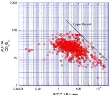
equivalent to applied pressure for permanent gases at lower pressures. The performance of new materials is often measured on a so-called Robson upper bound plots. A typical such plot is shown in Figure 3.2. The aim is to produce materials, which lie on or above the upper-bound line giving higher selectivity as well as permeability constant.
Figure 3.2 Upper bound correlations of carbon dioxide and nitrogen selectivity and
As is obvious from the above graph there are not too many materials exceeding the upper bound line. However, plotting permeation data this way allows quick screening for identification of potentially good membrane materials. Furthermore, one has to exercise caution for selecting the material for gas separation membranes from new material as sometime the permeability and selectivity measurements on pure materials do not lead to high performance membranes (Zhu, 2006).
3.2.2
Reverse Osmosis
Reverse osmosis membranes have been available for commercial use in desalination and wastewater treatment for a long time. For salt rejection most manufacturers provide data for feed containing 2,000 mg per litre salt at a trans-membrane pressure of 1.55 MPa. In addition to salt rejection, other parameters to consider are the compaction of the membrane due to high applied pressure, fouling of the asymmetric layer by feed components, tolerance of the material for extremes of pH and aggressive chemicals such as solvents and oxidants.
One of the major problems facing industrial application of reverse osmosis for water treatment is the fouling of membranes with biofilms. In addition to using frequent cleaning procedures, membrane surface modification to discourage the adhesion of biofilms to membrane surface has been used (Kutowy and Striez, 2003).
Several experimental procedures have been reported for characterizing the RO membranes. One very interesting protocol has been reported (Gupta et al., 2007) which utilizes Spiegler–Kedem membrane-transport model based on irreversible thermodynamics. This model was combined with FilmTheory description of the concentration polarization and was able to predict the total volumetric flux and intrinsic rejection over a range of feed concentration, flow rates, and transmembrane pressures. However, the model was applicable to dilute aqueous salt solutions only.
3.2.3
Nanofiltration
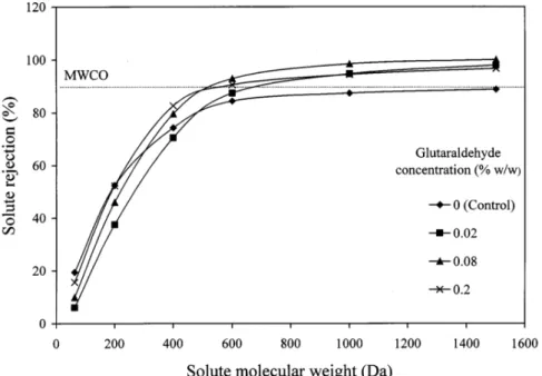
Nanofiltration membranes are sometimes described as being in between reverse osmosis and ultrafiltration membranes. However, nanofiltration membranes are distinct in terms of characterization through their propensities for rejection of charged and neutral species. Therefore the performance of membranes will be influenced by charge parameters also. In addition to the data on the rejection of solutes of lower molecular weight (less than 1000 Dalton, e.g. sugars, dyes), mono and multivalent ion rejection data is also important. Furthermore, the surface charge of the membranes plays an important role in the selection of test solutes and interpretation of the data. A typical molecular weight cut off (MWCO) curve showing retention of different membranes is shown in Figure 3.3 (Musale and Kumar, 2000).
Nanofiltration membranes often show solute rejection behaviour, which is dependent on the flux or applied driving forces and eventually reaches a limiting value (Marcel et al., 2005). Nanofiltration membranes reject salts on the basis of the valances of ions. Therefore rejection for salts such as sodium chloride, sodium sulphate and magnesium chloride is also determined. In order to determine charge characteristics, surface properties such as contact angel, zeta potential and atomic force spectroscopy are also used to characterize nanofiltration membranes.
Figure 3.3 Solute rejection curves for various nanofiltration membranes with low
molecular weight solutes. MWCO = Nominal Molecular Weight Cut-off (MWCO), which is defined as the molecular weight of the solute retained at a higher than 90% (w/w) level by the membrane.
3.2.4
Ultrafiltration
One of the most important properties of the ultrafiltration membranes is its permeation or sieving characteristics. Membrane manufacturers and researchers have used different test solutes and techniques to provide a rating of the sieving properties of the membranes. Generally, solutes such as polyethttlene glycol (PEG), dextrans and polyethylene oxide (PEO) are used as test solutes for characterizing the membranes. The procedure involves determination of the rejection by membrane of solutes of varying molecular weight at constant pressure and constructing a sieving curve (similar to Figure 3.3) to estimate the MWCO of the membrane. For example, for the curve shown with
solid squares a value of 650 Dalton is determined, which corresponds to higher than 90% rejection from Figure 3.3.
The pore size distribution of ultrafiltration membranes could be determined by a modified bubble-point method described by Capannelli et al. (1983). In brief, water saturated i-butanol was used to displace water in pre-wetted membranes with a constant increment of pressure. The pore radii (rpj) and the number of pores (nj) were determined
using Cantor's (eq. 3.4) and Hagen-Poiseuille's (eq. 3.5) equations, respectively:
=
(3.4)
= −
(
3.5)where , , , d, P and Q are the water/water saturated i-butanol interfacial tension, water/polymer contact angle, liquid viscosity, pore length, which is taken to be the membrane skin layer thickness, applied pressure and the permeate flow rate, respectively. A pore size distribution of laboratory scale for several ultrafiltration membranes has been reported using this method (Musale et al., 1999).
Both of the above methods require a large series of experiments. Researchers have reported techniques such as gel permeation chromatography (Nobrega et al., 1989) and field-emission electron microscopy ultrafiltration membranes and rejection of dextran of different molecular weights (Wickramasinghe et al., 2009) for determining the MWCO of membranes.
3.2.5
Microfiltration
Membrane properties such as pore sizes and distribution, number of pores per unit surface area and the bulk porosity are important for ascertaining the performance of a microfiltration membrane in an application. Membrane manufacturers use different techniques to test the membranes, therefore it is important that in selecting membranes for an application some standardized tests be performed. One of the most widely used tests for microfiltration membranes is bubble point determination. Other methods such as electron microscopy and direct challenging of the membranes with species of known sizes are also used.
Bubble point method requires that membrane be exposed to a wetting liquid where the liquid enters the pores due to capillary action. A gradual pressure applied to force the liquid through microfiltration membrane will result in the appearance of an air bubble, this pressure is correlated to largest pore in the membrane by Cantors’s equation.
= 4 () (3.6) where P is the pressure at which bubble appears, is solvent/air surface tension, is solvent-solid material contact angle and D is the diameter of the capillary pore. It is obvious from the above equation that liquids of higher surface tension such as water will require higher pressure to make the bubble for a given pore size. A very high pressure may cause deformation of the pores. Therefore, liquids of lower surface tensions such as isopropyl alcohol are often used for this test. Pore size distribution could also be determined by selecting suitable liquids and by increasing the pressure in small steps and correlating the increased flow with opening of additional pores of smaller sizes. Other techniques using air flow permporometry and thermoporometry have also been reported. However the big challenge remains to correlate the pore size distributions determined with different methods.
3.3
Separation Mechanisms for Different Membrane Processes
There are several different mechanisms of transport through membranes. These are dependent on membrane-type, operating conditions and the interacting parameters. Microfiltration and ultrafiltration processes are mainly characterized by size exclusion of the larger specie such as solute. In the case of reverse osmosis, nanofiltration and gaseous separation, diffusion of species also play a very important role, in addition to size exclusion. In this section, specific transport models and the phenomena of concentration polarization are discussed as it applied to different type of membrane processes.
3.3.1 Gas and Vapour Permeation
Permeation of gases through polymeric membranes is dependent on the structure of the material operating conditions and the gas-membrane material interactions. A good review of the historical perspective is given by Stannett (1978). The gas permeation behaviour is described by two distinct mechanisms described below:
3.3.1.1 Solution Diffusion Model
The first proponent of the concept of free-volume was Fujita (1968). Later several workers applied this to gaseous separation and beyond. Vrentas and Duda (1986) suggested that there are three components to the specific volume of polymer, namely occupied volume, interstitial and hole free volume. Considering that random movement allows the diffusion and transport of gaseous molecules, Stern et al. (1983) proposed that flux J and fractional free volume Vfcould be expressed as follows:
=
(
3.7)= + ∆ ( − ) − ∆ ( − ) +
(
3.8)where D and φ are diffusion coefficient and volume fraction of the gas in the polymer. Also , Tsand psare free volume, glass transition temperature and reference pressures
while terms Δα and Δβ relate to thermal expansion coefficient and compressibility. The mobility and mass fraction of the interacting gas is related to diffusion by the following expression (Koros and Hellums, 1989)
= (1 − ) (3.9)
where R, T, ui and wi are gas constant, temperature, gas mobility and mass fraction of
the gas, respectively. By combining the above equations and using a regression technique, Jordon and Koros (1990) determined various coefficients for transport of various gases in polymer and provided explanation of experimentally observed behaviour.
3.3.1.2 Pore Flow Model
Gas permeation through polymeric membranes could be treated as flow through porous media. This model first considers the contributions from Knudson diffusion, slip, viscous and surface transport and finally relates to preferential sorption capillary flow phenomena. It is assumed that fluid will show either great influence of interacting forces (in the pore) or free from interacting forces (bulk). The flow through the pore will depend on the mean-free path (λ) gas relative to the pore size. A polymeric membrane as a porous material will have a pore size distribution, and therefore, the overall flow will have contributions through various mechanisms. Flow mechanism for pores that are 0.05, 0.05–50 and larger than 50 times of mean free path will belong to Knudsen, slip and viscous flow. Mathematical forms of flux contributions are described in details in a text book (Matsuura, 1993). The gas flow flux (Qg) and various components are
presented as follows:
= / (3.10)
where Qk, M, R, T, R, (p2–p3) and δ are Knudsen flux, molecular weight of gas, gas
constant, temperature, pore radius, pressure differential and effective pore length, respectively;
= ( / )
(
3.11) where Qslis slip flow;=
( )(
3.12)where Qvis viscous flow; and
= + + (3.13)
However the flow of absorbed molecules on the surface of the pores will be governed by a different mechanism and called surface flow (Qs). The mathematical expression for Qs
has been reported in the literature (Rangarajan et al., 1984) as follows:
= ( − ) (3.14)
where Qs, ρapp, KHand p are surface flow, density, partition coefficient and pressure. The
term I4 and I5 are related to pores and are described in the literature (Rangarajan et al.,
1984).
The total gas flow is the sum of the gas phase flow (Qg) and pore surface flow
(Qs). The mathematical form of the above equations have firm thermo-chemical basis
and experimental data collected on different gases on polymeric membranes was modeled. Flow contributions of different types were estimated and correlated to the experimental observations.
3.3.2
Reverse Osmosis and Nanofiltration
Based on the extensive data in the literature, reverse osmosis flow models are based on homogeneous membranes, pore-based models and phenomenological models. Considering that nanofiltration membranes often have surface charges, flow through these membranes is described using Donnan exclusion principles. Assuming that top asymmetric thin layer of commercial membranes is responsible for permeation properties and support layer does not contribute to the rejection, various models are described below:
Solution diffusion model was first reported by Lonsdale et al. (1965) for sodium chloride water separations with cellulose acetate membranes. This model assumes that based on the chemical properties of solute and solvent, each one dissolve in the polymeric matrix to a different extent. Water flux through the membrane is described in the literatures (Ho and Sirkar, 1992) as follows:
= (∆ − ∆ )
(
3.15)where Pw, l, Δp and Δπ are water permeability, membrane active layer thickness,
pressure difference and osmotic pressure difference, respectively. Similarly, solute flux (Js) is given as:
= ( − )
(
3.16)where Ps, , and are solute permeability, solute concentration in the feed and
permeate, respectively. By combining the above equations, intrinsic solute rejection by the membranes could be defined as follows:
= / (3.17)
There are newer models (Pusch, 1986) capable of predicting even negative rejection, which the above model cannot do.
3.3.2.2 Pore Flow Models
In this model it is assumed that both surface phenomena and transport through the pores determine the solute rejection by the membrane. The model was first proposed by Sourirajan (1970). Membrane properties are such that preferential adsorption of the solute/solvent takes place on the walls of the pores while solute is being repelled at the same time. Solvent forming layers on the pore walls is pushed through the membrane. Solvent flux (Nw) through the membrane is given as follows:
= [∆ − { ( ) − ( )}]
(
3.18)where A, Δp, π(xs) are the pure water permeability constant, pressure difference and
osmotic pressures due to the difference between mole fractions of the solute in feed and permeate. Similarly, solute flux (Ns) is expressed as
where CT, Ks, Dsm, and are total molar concentration, solute distribution
coefficient, solute diffusion coefficient in the membrane , mole fractions of the solute in feed and permeate, respectively. A quantitative representation of this model known as the surface force pore flow model was later developed (Matsuura and Sourirajan, 1981), which allowed the incorporation of membrane as a function of pore size distribution.
3.3.2.3 Irreversible Thermodynamics Models
Using phenomenological transport equations, Kedem and Katchalski (1958) developed these models for dilute solutions. Solvent (Jw) and solute flux (Js) are
expressed as follows:
= (∆ − ∆ ) (3.20)
= ( ) (1 − ) + ( − ) (3.21)
( ) = (3.22)
where is reflection coefficient of membrane to solute and other symbols have the same meaning as before. It is interesting to note that in the event of no flow coupling, i.e., = 1, the above equations become identical to the solution-diffusion model.
3.3.2.4 Donnan Equilibrium and Nernst-Planck Models
As a charged membrane comes in contact with a salt solution, the ions of opposite sign of the membrane surface charge achieve membrane concentration, which is higher than bulk concentration. On the other hand, ions with the same charge as the membrane do not accumulate in the membrane to a very significant extent. This results in the creation of a Donnan potential. Further, applied pressure in membrane separations forcing water through the membrane also creates a potential. In order to maintain the electro-neutrality, both ions are rejected by the membrane. The salt (MzyYzm)
distribution coefficient (K*) is given by the following equation (Ho and Sirkar, 1992):
∗= =
∗
/
(3.23) where zi represents the charge of species i, cy and cy(m) are the concentrations of ions
having same and opposite charge of the membrane surface, respectively. , m and ∗
applicable to the nanofiltration membranes. Ion rejection ( ′) by the membrane is represented as follows (Bhattacharyya and Cheng, 1986):
= 1 − ∗ (3.24)
This model shows that the ion rejection is a function of membrane charge capacity, solute concentration and ionic charges. However, this model is qualitative in nature and does not consider the effects of diffusive and convective permeations. Other workers (Lakshminaranaiah, 1969; Dresner, 1972) have used a Nernst-Planck equation, which accounts for the convective and diffusive contributions to permeation in addition to the contributions from the Donnan equilibrium.
3.3.3
Ultrafiltration and Microfiltration
Under ideal conditions (steady state flow, laminar flow, negligible end effects, for Newtonian flow) such as a macromolecule solution permeating through membranes, the flux (J) is usually expressed by Hagen-Poiseuille equation given below:
J=ϵ dp 2∆P
32 ∆x μ (3.25)
where ε, dp, ΔP, Δx, and µ are surface porosity of membrane, pore diameter,
trans-membrane pressure, length of trans-membrane pore and fluid viscosity, respectively. In most applications, the osmotic pressure exerted by large molecules is normally neglected. As the filtration process operates more solute is depleted from feed solution near the surface of the membrane. Over time the solute concentration near the surface will be significantly higher than the bulk solute concentration. This leads to the formation of a so-called concentration polarization layer, which offers resistance to the permeation of the solvent. Depending upon the nature of the solute, this layer might turn into a gel-like substance and offer even greater resistance. Irrespective of the mechanism of formation, it provides a clear hydrodynamic resistance to permeation of the solvent through the membrane. It is possible that solute concentration in this layer might stabilize due to back diffusion in the bulk of the feed solution. By changing experimental conditions such as increased cross flow velocity, resistance due to concentration polarization could be reduced.
In a system where permeation is pressure independent, one can use a film theory-based analysis for modelling the flux. During filtration the solute is brought to the surface of the membrane via convective flow and solute concentrating in the boundary layer diffuses back to the bulk. By combining these two processes one can express the flux in terms of solute concentration, diffusion coefficient and mass transfer coefficient (Cheryan, 1998) as follows:
= ln = ln
(
3.26) where D, δ, C and k are diffusion coefficient, polarization layer thickness, solute concentration and mass transfer coefficient, respectively. Subscripts G and B are for concentrations in polarization layer and in the bulk.There are a number of correlations available in the literature to calculate mass transfer coefficient. The following correlations of dimensionless numbers (Hwang and Kammermeyer, 1975) are used for different fluid flow conditions.
For laminar flow conditions (Reynolds number, Re <1800)
ℎ = = 1.86 . . ( ) . (3.27)
For turbulent flow (Re > 4000)
ℎ = = 0.023 . .
(
3.28)where Sh, Sc, dhand L are Sherwood number, Schmidt number, hydraulic diameter and
channel length, respectively.
The above description of flow through membranes is valid for conditions where operation is pressure independent. However, it is important to study the pressure effects for real applications. One of the approaches uses the resistance-in-series model, which is often used in heat transfer studies. Here flux is expressed using the following generalized relation:
= ∆ = ∆
(
3.29)where Rm, Rfand Rgrepresent resistances due to membrane, fouling and concentration
polarization, respectively. By collecting flux data at varying pressures, solute concentrations and cross-flow velocities, one can determine the values of resistances and identify the optimal operating parameters.
3.4
Modelling and Simulation in Membrane Separation Processes
Modelling and simulation techniques have been applied in the development of membrane technology at several different levels. Extensive modelling studies have
focused on the formation of the membranes and solvent-solute interactions, which are discussed in previous two sections. In this section, the focus is on application of Computational Fluid Dynamics (CFD) studies in understanding the flow behaviour in membrane modules, with potential of developing better products.
Design and deployment of membrane-based processes for industrial application requires lot of development work including the use of reliable computational methods. Modelling techniques such as CFD has the potential to provide a lot of relevant information with comparatively smaller sets of experimental data. Furthermore, a tremendous access to computing power for little investment has made completion of large computations easier. It has also allowed calculation of important parameters such as shear-stress and strains, which are not easy to determine experimentally.
In order to simulate the flow behavior, the conservation equation for mass and momentum are first solved using finite volume method. If needed, a set of species conservation equations are solved to account for the separation. The governing equations, based on the physical principles of continuity, momentum conservation and solutes conservation are set in three-dimensional domain to examine the fluid flow characteristics and concentration profiles of the species. Non-slip boundary conditions at wall surface and variation in solute concentration are included in the compressible solver as well. The boundary conditions are defined next, and the model development and simulations are performed using commercial CFD software. The fluid properties are defined before executing the simulation loop. Operating parameters, such as mass flow rate, pressure and species concentrations are obtained and implemented as boundary conditions from empirical data. The simulations are performed using various options such as unsteady-laminar flow conditions at ambient temperature. The discretization of the governing equations is accomplished using a segregated compressible flow solver in which each governing equation is solved separately. In order to satisfy continuity equations the Semi-Implicit Method for Pressure-Linked Equations (SIMPLE) formulation of pressure-velocity coupling might be used. In order to update the velocity field, the three-dimensional (3D) Navier-Stokes equations are solved using current values for pressures and face mass fluxes in the considered vessel. The convergence criteria for the continuity and velocity parameters are the fixed usually at 0.001%.
The dimensions of the computational domain are identical with that of the vessel considered. A commercial grid generation software is often used to generate the 3D geometry and mesh for CFD studies. An effort is usually made to implement the structured and uniform grid for the entire geometry for numerical advantage. In order to accomplish this, the geometry is decomposed in such way that different scheme can be implemented for all the segments of complex portions. Structured meshing is performed to divide the fluid flow domain in to sub-domains and hexahedral cells and the discretized governing equations are solved inside each cell. The continuity and
momentum equations across the common interfaces between two sub-domains, the feed and the permeate side in a membrane system are solved to visualize fluid flow in the entire domain. The membrane in the domain is usually defined as shadowed wall, while all other walls represent the barriers of the remaining cell geometry. Grid refinement is performed to achieve grid independence by analyzing the concentration gradient within the geometrical domain. For specific calculation outside the commercial software one can use the option of User Defined Functions.
In this paragraph several examples are reviewed to show the potential of CFD techniques in membrane technology. Ghidossi et al. (2006) have published a comprehensive review of CFD techniques relevant to the development of membrane science and technology. They have emphasized different computations, which will help to enhance the membrane performance through advanced understanding of hydrodynamic and fouling characteristics over membranes and inside the modules. Furthermore, CFD techniques allow combination of filtration and hydrodynamic models, which leads to even better understanding suitable for membrane-based application development. Marriot and Sorensen (2003) studied flow in hollow fiber and spiral modules by combining Darcy’s equation with Navier-Stokes equations. Their experimental results matched with the models. A more comprehensive model, which could predict the flow behavior in the vicinity of the porous surface with variable permeability (Das et al., 2002) was reported. A lot of work has been reported on impact of physical processes on the flow in membrane slits or spirals, where circulating flows are often in laminar range (Geraldes et al., 2002). A general purpose CFD model was proposed by Wiley and Fletcher (2003), which combined the concentration polarization phenomena with the hydrodynamics characteristics and was verified experimentally. Although most of the studies are reported for laminar conditions, there were some attempts to study the ultrafiltration process in turbulent regimes (Pellerin et al., 1995).
One of the most important applications of CFD techniques for membrane technology is in advancing our understanding of the complex hydrodynamics encountered in gas sparging, insertion of spacers as turbulence promoter, generation of Dean and Taylor vortices and special geometries in modules. In order to restore declining performance of membranes caused by concentration polarizing and fouling, one has to resort to mechanical means as the chemical cleaning generally needs to be avoided due to obvious reasons. Stanton et al. (2002) reported a CFD technique where contribution of the air bubbles to flux enhancement could be directly correlated to the formation vortices. The role of spacers in membrane modules is to enhance performance by promoting turbulence and disrupting the formation of concentration/fouling layers. However, use of such devices is associated with increased pressure drop and flow mal-distribution in the module. Several experimental (Da Costa et al. 1991, 1994; Li et al., 2004) as well as CFD studies (Karode and Kumar, 2001; Cao et al., 2001; Schiwinge et al., 2002) have been reported. CFD studies have focused on ascertaining the effects of
different geometric arrangements of the spacers in thin channels and their impact on improving the hydrodynamic conditions in the module. Karode and Kumar (2001) evaluated the flow patterns of various commercial spacers (e.g., Figure 3.4) and established a relationship between spacer properties shear stress and drag coefficients.
Figure 3.4 Velocity vectors for NALTEX-56 spacer for an inlet velocity of 1 m/s.
CFD studies for different membrane geometries such as tubular membranes with inserts (Bellhouse et al., 2001), rotating membranes (Serra and Wiesner, 2000) and spiral membranes (Ranade and Kumar, 2006a, 2006b) have also been reported. In all studies CFD revealed valuable information on distribution of shear stress and other flow behavior, which could be used in designing applications. A typical shear stress distribution in a spacer domain for flat and curved channels is shown in Figure 3.5 (Kumar and Ranade, 2006b).
Figure 3.5 Contours of all shear stress in flat and annular channels (red = 6.2 Pa; blue
CFD studies have firmly established the relationships between shear stress values and fouling propensities as well as allowed the development of newer products such as high performance spacers.
3.5
Future Perspectives
Membranes are fabricated with a variety of materials including polymers, ceramics and metals. Each of the material choice has its advantages and disadvantages. This area of research continues to produce enormous literature. Most of this research focuses on material properties that are potentially beneficial for making a high performance membrane. In future efforts will be made in producing membranes from mixed matrix materials such as combination of polymers and inorganic materials. Additional research will focus on making the ingredients of mixed materials membranes compatible by physical and chemical techniques. There has been large number of laboratory scale studies on membranes containing active components such as silver salts for certain separation to enhance the performance. Research efforts will focus on making industrial scale membranes containing these active ingredients.
Membranes are fabricated in various formats such as flat sheets and hollow fibers using phase inversion techniques involving gelation or thermal techniques. Most commercial membranes are made using the gelation techniques, which produce large amounts of wastewater containing solvents and additives. New membrane fabrication schemes will focus on recycling wastewater and minimizing the amount of waste streams.
Membrane separation mechanisms have mainly focused either on diffusion or pore flow concepts, which provide reasonable explanation in most cases. In the future researchers will focus on unifying these broad concepts with supports from additional experiments designed to measure the detailed properties of the membranes and their interaction with feed components. Our knowledge of phenomena such as concentration polarization will be further advanced with the help of in-situ measurements of the concentration of species in the feed.
The membranes module design and its efficient use plays an important role in a membrane-based separation scheme. With the easy access to computer-intensive techniques such as Computational Fluid Dynamics, tremendous efforts will be made to understand the fluid flow behaviour in modules and its relationship with the performance of the module. Extensive use of these computational techniques will lead to improved products. One of the major challenge in membrane applications is the detrimental impact of fouling on the performance of the membranes. Researchers have
tried different techniques to mitigate the problem. Newer techniques including new fouling-resistant membranes will be developed in combination with improved process control to minimize fouling related performance decline.
Membrane-based application in certain industries such as drinking water, water recycling, dairy and energy are well-established. However their penetration in energy intensive chemical process and petroleum industry has been slow. New membranes processes deploying new membranes will be developed especially in the non-traditional applications involving challenging feeds containing solvents, corrosive chemicals and oxidants. In order for the membrane-based application to be adopted in wide ranging industries, newer studies will focus on extensive process simulation including the comparison with the existing technologies. A detailed energy and mass balance combined with economic analysis will help industry to adopt membrane-based separation schemes.
3.6
Summary
This chapter describes all important aspects of a membrane-based separation process. After a brief introduction properties of membrane materials and their relevance for gaseous and liquid separation are described in details including the specific information relevant for gas-vapour, reverse osmosis, nanofiltration, ultrafiltration and microfiltration processes. Currently used separation models based on solution diffusion and pore flow are described for different type of membrane processes including the applicable mathematical equations. Use and potential application of Computational Fluid Dynamics techniques in developing improved products and enriching understanding of flow behaviour, has also been included. The Chapter closes with a brief description of future directions in the membrane technology and its industrial applications.
3.7
References
Bellhouse, B.J., Costigan, G., Abhinava, K., and Merry, A. (2001). “The performance of helical screw-thread inserts in tubular membranes.” Sep. Purif. Technol., 22–23, 89–113.
Bhattacharyya, D., and Cheng, C. (1986). “Separation of metal chelates by charged composite membranes.” In Recent Developments in Separation Science, Li, N.N. (ed), vol. 9, p. 907, CRC Press, Boca Raaton, FL, USA.
Cao, Z., Wiley, D.E., and Fane, A.G. (2001). “CFD simulation of net-type turbulence promoters in narrow channel.” J. Membr. Sci., 185, 157–176.
Capannelli, G., Vigo, F., and Munari, S. (1983). “Ultrafiltration membranes: Characterization methods.” J. Membr. Sci., 15, 289–313.
Charcosset, C., and Bernengo, J.-C. (2000). “Characterization of microporous membranes using confocal scanning laser microscopy in fluorescence mode.” Eur. Phys. J. Applied Physics, 12, 195–199.
Cheryan, M., (1998). Ultrafiltration and Microfiltration Handbook. Technomic Publishing Company Inc., Lancaster, PA, USA.
da Costa, A.R., Fane, A.G., Fell, C.J.D., and Franken, A.C.M. (1991). “Optimal channel spacer design for ultra-filtration.” J. Membr. Sci., 62, 275–291.
da Costa, A.R., Fane, A.G., and Wiley, D.E. (1994). “Spacer characterization and pressure drop modelling in spacer-filled channels for ultra-filtration.” J. Membr. Sci., 87, 79–98.
Das, D.B., Nassehi, V., and Wakeman, R.J. (2002). “A finite volume model for the hydrodynamics of combined free and porous flow in sub-surface regions.” Adv. Environ. Res., 7, 35–58.
Dresner, L. (1972). “Some remarks on the integration of the extended Nernst-Planck equations in the hyperfiltration of multicomponent systems.” Desalination, 10, 27–46.
Fujita, H. (1968). “Organic Vapors above the Glass Transition Temperatures.” In Diffusion in Polymers, Crak, J., and Park, G.S. (eds.), Academic Press, New York, NY, USA.
Geraldes, V.M., Semiao, V., and de Pinho, M.N. (2002). “The effect on mass transfer of momentum and concentration boundary layers at the entrance region of a slit with a nanofiltration membrane wall.” Chem. Eng. Sci., 57 735–748.
Ghidossi, R., Veyret, D., and Moulin, P. (2006). “Computational fluid dynamics applied to membranes: State of the art and opportunities.” Chemical Engineering and Processing, 45, 437–454.
Gupta, V.K., Hwanga, S., Krantz, W.B., and Greenberg, A.R. (2007). “Characterization of nanofiltration and reverse osmosis membrane performance for aqueous salt solutions using irreversible thermodynamics.” Desalination, 208, 1–18.
Ho, W.S.W., and Sirkar, K.K. (1992). Membrane Handbook, Chapman and Hall, New York, NY, USA.
Hwang, S., and Kammermeyer, K. (1975). Membranes in Separations, John Wiley, New York, NY, USA.
Jordon, S.M., and Koros, W.J. (1990). “Permeability of pure and mixed gases in silicone rubber at elevated pressures.” J. Polymer Science, Polymer Physics Edition, 28, 795–809.
Kedem, O., and Katchalski, A., (1958). “Thermodynamic analysis of the permeability of biological membranes to non-electrolytes.” Biochim. Biophys. Acta, 27, 229– 246.
Koros, W.J., and Chern, R.T., (1987) Separation of gaseous mixtures using polymer membranes. In Handbook of Separation Process Technology, Ed. Rousseau, R.W., pp. 862-953, John Wiley & Sons, New York, NY, USA.
Koros, W.J., and Hellums, M.W. (1989). Transport Properties, Encyclopedia of Polymer Science and Engineering, 2nd ed. (supplement volume), pp 724–802, John Wiley and Sons, New York, NY, USA.
Kurdi, J., and Kumar, A. (2006). “Formation and thermal stability of BMI-based interpenetrating polymers for gas separation membranes.” J. Membrane Sci., 280, 234–244.
Kutowy, O., and Striez, C. (2003). “Intrinsically bacteriostatic membranes and systems for water purification.” US Patent No. 6,652,751.
Lakshminaranaiah, N. (1969). Transport Phenomena in Membranes, Academic Press, New York, NY, USA.
Li, F., Meindersma, W., de Haan, A.B., and Reith, T. (2004). “Experimental validation of CFD mass transfer simulations in flat channels with nonwoven net spacers.” J. Membr. Sci., 232, 19–30.
Lonsdale, H., Merten, U., and Riley, R. (1965). “Transport properties of cellulose acetate osmotic membranes.” J. Appl. Polymer Sci., 9, 1341–1362.
Marriott, J., and Sorensen, E. (2003). “A general approach to modelling membrane modules.” Chem. Eng. Sci., 58, 4975–4990.
Matsuura, T., and Sourirajan, S. (1981) “Reverse Osmosis transport through capillary pores under the influence of surface forces.” Ind. Eng. Chem., Process Des. Dev., 20, 273–282.
Matsuura, T. (1993). Synthetic Membranes and Membrane Processes, CRC Press Inc. Boca Raton, FL, USA.
Mulder, M.H.V., van Voorthuizen, E.M., and Peeters, J.M.M. (2005). Membrane Characterization in Nanofiltration–Principles and Applications, Schafer, A.I., Fane, A.G., and Waite, T.D. (eds.), Elsevier, Oxford, UK, p98.
Musale, D.M., Kumar, A., and Pleizier, G. (1999). “Formation and characterization of poly(acrylonitrile)/chitosan composite ultrafltration membranes.” J. Membr. Sci., 154, 163–173.
Musale, D.M., and Kumar, A. (2000). “Effects of surface crosslinking on sieving characteristics of chitosan:poly(acrylonitrile) composite nanofiltration membranes.” Separ. Purif. Technol., 21, 27–38.
Nobrega, R., de balmann, H., Aimar, P., and Sanchez, V. (1989). “Transfer of dextran through ultrafiltration membranes: a study of rejection data analysed by gel permeation chromatography.” J. Membr. Sci., 45, 17–89.
Pellerin, E., Michelitsch, E., Darcovich K., Lin, S., and Tam, C.M. (1995). “Turbulent transport in membrane modules by CFD simulation in two dimensions.” J. Membr. Sci., 100, 139–153.
Pusch, W. (1986). “Measurement techniques of transport through membranes.” Desalination, 59, 105–198.
Ranade, V.V., and Kumar, A. (2006a). “Fluid dynamics of spacer filled rectangular and curvilinear channels.” Journal of Membrane Science, 271, 1–15.
Ranade, V.V., and Kumar, A. (2006b). “Comparison of flow structures in spacer-filled flat and annular, channels.” Desalination, 191, 236–244.
Rangarajan, R., Majid, M.A., Matsuura, T., and Sourirajan, S. (1984). Permeation of pure gases under pressure through asymmetric porous membranes. Membrane characterization and prediction of performance” Ind. Eng. Chem., Proc. Des. Dev., 23, 79–87.
Robeson, L.M. (2008). “Upper bound revisited.” J. Membr., Sci., 320, 390–400.
Schiwinge, J., Wiley, D.E., and Fletcher, D.F. (2002). “Simulation of the flow around spacer filaments between narrow channel walls. 1. Hydrodynamics.” Ind. Eng. Chem. Res., 41, 2977–2987.
Serra, C.A., and Wiesner, M.R. (2000). “A comparison of rotating and stationary membrane disk filters using computational fluid dynamics.” J. Membr. Sci., 165 19–29.
Sourirajan, S. (1970). Reverse Osmosis, Academic Press, New York, NY, USA.
Stannett, V. (1978). “The transport of gases in synthetic polymeric membranes-an historic perspective.” J Membr. Sci., 3, 97–115.
Stanton, S., Taha, T., and Cui, Z. (2002). “Enhancing hollow fibre ultrafiltration using slug-flow a hydrodynamic study.” Desalination, 146, 69–74.
Stern, S.A., Kulkarni, S.S., and Frisch, H.L. (1983). “Test of a free volume model for gas permeation through polymer membranes. I Pure CO2, CH4,C2H4and C3H8 in
polyethylene.” J. Polymer Sci., Polymer Physics Edition, 21, 467–481.
Ulbricht, M., and Belfort, G. (1996). “Surface modification of ultrafiltration membranes by low temperature plasma II. Graft polymerization onto polyacrylonitrile and polysulfone.” J. Membr., Sci., 111, 192–215.
Vrentas, J.S., and Duda, J.L. (1986). “Diffusion.” In Encyclopedia of Polymer Science, Kroschwitz, J.I. (ed.), 2nd ed., Vol. 5, pp 36–68, John Wiley and Sons, New
York, NY, USA.
Wickramasinghe, S.R., Bower, S.E., Chen, Z., Mukherjee, A., And Husson, S.M. (2009). “Relating the pore size distribution of ultrafiltration membranes to dextran rejection.” J. Membr., Sci., 340, 1–8.
Wiley, D.E, and Fletcher, D.F. (2003). “Techniques for computational fluid dynamics modelling of flow in membrane channels.” J. Membr. Sci., 211, 127–137.
Zhu, Z. (2006). “Permeance should be used to characterize the productivity of a polymeric gas separation membrane.” J. Membr., Sci., 281, 754–756.