Development of an open source software library for solid oxide fuel cells

https://doi.org/10.4224/21268547

READ THESE TERMS AND CONDITIONS CAREFULLY BEFORE USING THIS WEBSITE.

https://nrc-publications.canada.ca/eng/copyright

Vous avez des questions? Nous pouvons vous aider. Pour communiquer directement avec un auteur, consultez la

première page de la revue dans laquelle son article a été publié afin de trouver ses coordonnées. Si vous n’arrivez pas à les repérer, communiquez avec nous à PublicationsArchive-ArchivesPublications@nrc-cnrc.gc.ca.

Questions? Contact the NRC Publications Archive team at

PublicationsArchive-ArchivesPublications@nrc-cnrc.gc.ca. If you wish to email the authors directly, please see the first page of the publication for their contact information.

For the publisher’s version, please access the DOI link below./ Pour consulter la version de l’éditeur, utilisez le lien DOI ci-dessous.

Access and use of this website and the material on it are subject to the Terms and Conditions set forth at

Development of an open source software library for solid oxide fuel

cells

Beale, S. B.; Roth, H. K.; Le, A.; Jeon, D. H.

https://publications-cnrc.canada.ca/fra/droits

L’accès à ce site Web et l’utilisation de son contenu sont assujettis aux conditions présentées dans le site

LISEZ CES CONDITIONS ATTENTIVEMENT AVANT D’UTILISER CE SITE WEB.

NRC Publications Record / Notice d'Archives des publications de CNRC: https://nrc-publications.canada.ca/eng/view/object/?id=ab243f2e-c463-4926-b007-486c56cafdd5 https://publications-cnrc.canada.ca/fra/voir/objet/?id=ab243f2e-c463-4926-b007-486c56cafdd5

and Environment et environnement

Process Engineering and Modeling Génie des procédés et modélisation

Development of an Open Source

Software Library for Solid Oxide Fuel Cells

S.B. Beale, H.K. Roth, A. Le, D.H. Jeon

Technical Report Rapport technique

2013/01

NRCC 53179

UNLIMITED ILLIMITÉE

EXECUTIVE SUMMARY

This report details the development of a Multi-Scale integrated fuel cell suite of software developed at NRC and Queens/RMC Fuel Cell Centre in conjunction with Forschungszentrum Jülich GmbH. Following the history of the project, some mathematical details of the cell/small stack level models are provided, together with brief details on other scale models. The model is developed for application to solid oxide fuel cells, though it may readily be applied to polymer electrolyte fuel cells. The implementation of the model into the C++ class library, OpenFoam, is then explained together with details of how to download and run the code from the repository where it resides. Some examples of practical applications, considered as validation and verification exercises of the code, together with discussion highlighting the advantages and disadvantages associated with the open source implementation, are provided. Finally, general conclusions from the project are drawn and suggestions for future work are proposed.

CONTENTS

Page

DEVELOPMENT OF AN OPEN SOURCE SOFTWARE LIBRARY FOR SOLID

OXIDE FUEL CELLS ...1

1. INTRODUCTION ...1

1.1 Historical Background...1

1.1.1 National Research Council ...1

1.1.2 Forschungszentrum Jülich GmbH ...2

1.1.3 Queen’s-RMC Fuel Cell Research Centre...2

1.1.4 Project meetings...2

1.2 Problem Definition ...3

1.3 Description of Remainder of the Report...3

2. Description of cell and small-stack model...4

2.1 SOFC cell-level model equations ...4

2.1.1 Transport equations...4

2.1.2 Porous media source term ...5

2.1.3 Species source terms ...5

2.1.4 Electrochemistry ...7

2.1.5 Area specific resistance...7

2.1.6 Activation overpotentials...8

2.1.7 Electrolyte heat source...8

2.1.8 Computational algorithm...9

2.2 Multi-scale models ...9

2.2.1 Stack model...9

2.2.2 Micro-scale model ...10

2.2.3 Two-potential model ...10

3. Implementation of model equations in C++ class library...11

3.1 Brief description of OpenFOAM code ...11

3.2 ‘Conjugate’ vs ‘cell’ models...11

3.3 Model development ...12 4. Operational details...13 4.1 Introduction...13 4.2 Prerequisites...13 4.2.1 OpenFoam ...13 4.2.2 svn...13

4.4 Directories ...15 4.4.1 trunk/src/...15 4.4.2 trunk/run/ ...15 4.5 Installation ...17 4.5.1 src...17 4.5.2 cases ...17

4.6 Running the model ...17

4.7 Mesh files ...18 4.8 Inputs...22 4.9 Outputs ...24 4.9.2 Run log ...25 4.10 Summary ...25 5. Case studies ...26 5.1 IEA geometry...26 5.2 Taiwan geometry ...26 5.3 Jülich F-design ...27 6. Discussion of results...30 6.1 Technical achievements ...30 6.2 Problems encountered...31

6.3 Suggestions for future work...32

7. Conclusions and recommendations...33

APPENDIX i: Specifying meshes for a new geometry ...34

LIST OF FIGURES

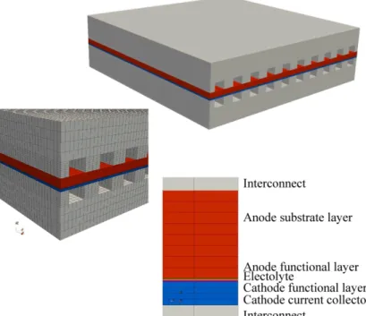
Figure 1. Schematic of fuel cell showing component layers... 5

Figure 2. Computer aided design geometry used to generate computational grid for Jülich F-design ...27

Figure 3. V-i performance curves, from ref. [19]...27

Figure 4. Air-side pressure...29

Figure 5. Plate temperature ...29

Figure 6. Air-side streamlines ...29

Figure 7. H2mass fraction...29

Figure 8. Local current density...29

Figure 9. Nernst potential...29

LIST OF TABLES Table Page Table 1. svn models...14

Table 2. Input properties and parameters ...20

Table 3. Input initial fields. ...21

Table 4. fvSchemes settings...22

Table 5. fvSolution settings...23

Table 6. Output files at times > 0. ...24

Table 7. Components commonly used in F-design stacks...28

DEVELOPMENT OF AN OPEN SOURCE SOFTWARE LIBRARY FOR SOLID OXIDE FUEL CELLS

1. INTRODUCTION 1.1 Historical Background

1.1.1 National Research Council

The National Research Council (NRC) is Canada’s premier federal science and technology laboratory. Within NRCs Institute for Chemical Process and

Environmental Technology (ICPET), now a unit of the Energy Mining and Environment (EME) portfolio, fuel cell models have been developed using computational fluid dynamics (CFD), and other codes and methods, since 1999. These include solid oxide fuel cell (SOFC) and polymer electrolyte fuel cell (PEMFC) models.

Originally, models were developed by writing subroutines and functions in-house, in programming languages such as FORTRAN and C, within large commercial codes such as PHOENICS and Fluent [1]. Subsequently with the development by Fluent and others, of their own specialized PEMFC and SOFC codes, the NRC-developed user-defined functions were abandoned. However, experience in adapting such “black-box” commercial CFD codes to the complex physico-chemical hydrodynamics associated with hydrogen fuel cells was mixed. In addition, because such codes are proprietary, ie. the property of the software house, it is not possible to share resources among collaborators and partners, without such third parties purchasing additional licenses at significant cost.

At the same time in-house codes were also developed, in C/C++. These have the advantage that the authors have complete control over the product, but suffer from the need for development of suitable interfaces to graphical post-processing software, such as VTK, and front-end graphical user interfaces (GUI) which can involve more work and maintenance than the development of the core solver itself. In addition, the issue of portability, eg between MSWindows and UNIX, is a matter for concern. Also NRC/ICPET does not have the facilities to provide software support, in the commercial sense, to partners and stakeholders. It became apparent that a third way was necessary; one where software development was restricted to features salient to fuel cell research and

development, but without “reinventing the wheel” in terms of well-established flow solvers and numerical schemes. The arrival of open source CFD codes in the workplace proved to be timely, and it was agreed to conduct an experiment in fuel cell modelling employing the open source CFD code “OpenFoam”, Weller et al. [2], which is the core activity of this program. In addition to this project,

NRC/ICPET.

1.1.2 Forschungszentrum Jülich GmbH

Forschungszentrum Jülich GmbH (FZJ) is one of Europe’s largest

interdisciplinary research centres, and generates research in the areas of health, energy, climate and information technology. The Institute for Energy Research – Fuel Cells (IEF-3), now including climate (klima) research (IEK-3, Energy

Process Engineering), has been developing fuel cell technology for a number of decades. It is generally considered to be the leading European laboratory in fuel cell development. FZJ has been a leading developer of planar SOFCs and is working on the development of high temperature polymer electrolyte fuel cells (HT-PEMFCs) and direct methanol fuel cells (DMFCs) . Similar to the NRC situation, FZJ had been employing commercial codes, but increasingly found the conventional licensing model to be, not only expensive, but also sub-optimal in the context of fuel cell R&D, especially for running in parallel on the Jülich

Supercomputing Facility, one of the largest supercomputing facilities in the world. 1.1.3 Queen’s-RMC Fuel Cell Research Centre

Although not formally part of the original project/contract between NRC and FZJ; faculty members, staff, and students at the Queen’s-RMC Fuel Cell Research Centre (FCRC) have participated in the project from its earliest stages, and will continue to do so into the future. The FCRC is Canada's leading university-based research and development organization in partnership with industry dedicated to advancing the knowledge base for addressing the key technology challenges to the commercialisation of fuel cell applications.

1.1.4 Project meetings

Dr. Beale visited IEF-3 Jülich in March 2007 where the idea for a project was originally conceived. M. Spiller and D. Froning of IEF-3 visited NRC in 6-7 September 2007. Dr. Beale visited Jülich together with Prof. Pharoah and Prof. Karan in December 2007. A MUSIC workshop was held in the Jülich

Supercomputing Centre in March 2009. In attendance were H. Jasak, H. Rusche (Wikki Ltd.), S. Beale, H. Roth (NRC), J. Pharoah, H-W Choi, D. Jeon (FCRC), D. Froning, S. Berns (FZJ). Dr. Beale and Prof. Pharoah visited Jülich and also Wikki in London 19-21 January 2011. The partners met again in Montreal in May 2011 at the ECS meeting. In addition to face-to-face meetings, video

conferences between the parties have been held on a monthly basis over the period of the project.

1.2 Problem definition

The partners agreed to develop a common framework for fuel cell modelling. The model was to be for Multi-Scale Integrated Fuel Cells (MUSIC), the ultimate goal being to develop an integrated suite of software, freely available to fuel cell researchers at every scale from nano/micro through to cell/stack and hotbox. By freely sharing the implementation, it is hoped to accelerate technical

improvements in fuel cell modelling and hence fuel cell design, eliminate silos, and establish a ‘community of users’ who can continually upgrade and enhance the MUSIC library. At the same time the details of any specific design can be kept private, thereby obviating any compromise to intellectual property to individual stakeholders, who may be potential business rivals, in the project. The authors will maintain versions using configuration management (CM) tools. The code is to run on PCs, parallel LINUX Beowulf clusters, and eventually super-computing facilities. The existing software suite, OpenFOAM, was selected as the platform for the project. Technical support was provided by Wikki Ltd. (London, UK) under sub-contract to NRC. Adoption of software best practices [3] from the outset assists in continuity in model development and application.

The details of the sub-component of the work statement specific to the NRC-Jülich funded interaction as discussed in this report are as follows: NRC staff and personnel would:

1. Implement a SOFC/HTPEMFC single-cell model in OpenFoam 2. Implement a SOFC/HTPEMFC stack model in OpenFoam 3. Perform simulation for a 3D Jülich fuel cell stack

4. Verify and validate the developed model(s)

Owing to staffing and funding issues at both NRC and FZJ, there were some variances from the original work statement as further detailed in the report below.

1.3 Description of remainder of the report

This report is mainly centred on the development, application, and

documentation of the cell-level and detailed (cell-based) stack model, in the context of SOFCs, since this consumed, by far, the majority of the actual time spent on the project. Chapter 0 gives a description of the cell/small-stack level model together with a brief description of MUSIC models at other scales. Chapters 2 and 0 discuss the specific implementation of the model in

OpenFOAM and also provide details for the user interested in downloading and running the cell-level code for the cases of co-flow, counter-flow, and cross-flow. The architecture for other MUSIC modules is similar to that provided here at the cell-level. Chapter 3 discusses some case studies considered as part of the validation and verification process. Finally, Chapter 4 contains a discussion of the overall results of the project and Chapter 5 points to some conclusions and

suggestions for future work.

Description of cell and small-stack model 1.4 SOFC cell-level model equations

The fuel cell is presumed to be composed of the following volumetric zones: two interconnects, fuel (channel), passive anode substrate layer (ASL), active anode function layer (AFL), electrolyte, cathode current collector (CCL), cathode

functional layer (CFL), and air (channel). The reactions in the active layers are presently being treated as acting on planar interfaces between the volumetric electrode(s) and the electrolyte.

A binary mixture of oxygen and nitrogen is presumed on the air (cathode) side, whereas a bindary mixture of hydrogen, and water vapour is presumed on the anode side.

1.4.1 Transport equations

The equations to be solved are as follows:

 

div  u 0 (1)









div uu  gradpdiv gradu S_P (2)









div uy_i div  grady_i (3)









Figure 1. Schematic of fuel cell showing component layers. 1.4.2 Porous media source term

In the , AFL, CFL, ASL, CCL

D k    P u S (5)

ie., the state variable is the superficial (not interstitial) velocity. 1.4.3 Species source terms

In the cell model, the electrochemical reactions are presumed to occur at the interface of the AFL and CFL with the electrolyte. This shortcoming will be

removed in future versions. The source terms are thus per unit area m (kg/m_i '' 2_s) (for H2, H2O and O2) and related to current density, i" (A/m2), according to

Faraday’s law. The mass source/sink terms are given by, " '' i Mi m F     (6)

where M = 2, 18 and 32 [kg/kmol] for H2, H2O, O2 and  = 2, 2, 4 [electrons transferred per molecule] respectively.

The species source terms per unit area, S , are prescribed as follows:'' Air-side (cathode): O2 mass sink 2 O 32 '' 4 i m F     (7) O2species sink:





H2species sink due to H2consumption





2 2

H H

'' " 1

S m_ y ₍₁₁₎

H2O species source due to H2consumption

O H H2" 2 '' m y S  (12) H2O mass source 2 H O 18 '' 2 i m F     (13)

H2O species source due to H2O production





2 2

H O H O

'' " 1

S m_ y ₍₁₄₎

H2species sink due to H2O production

2 2

H O H

" "

1.4.4 Electrochemistry

If the current density is considered variable, the cell voltage, V, may be expressed as, c a R i E V      (16)

where aand care anodic and cathodic overpotentials, and R is the area specific resistance(m2_).

The Nernst potential, E, is obtained as

a p p F RT x x x F RT E E _                 0 O H 0.5 O H 0 ln 4 ln 2 2 2 2 (17)

Where





where  is the reference Gibb’s free energy. From Hernández-Pacheco and G₀ Mann [4], the following expression is obtained.

 

1.4.5 Area specific resistance

Initially a semi-empirical correlation by Ghosh et al., see [5], was used to compute R in units of ohm cm2_.

2 3 4 0.3044 0.408 0.8687 2.7861 2.9285 R  r r  r  r (20) where 1463 . 1 1000   T r (21)

with T in degrees C. Other ASR correlations were subsequently coded based on (proprietary) formulations provided by FZJ, and others. These may, or may not, include an implicit contribution due to activation overpotentials being excluded explicitly from Eq. (16).

1.4.6 Activation overpotentials

The overpotentials are obtained implicitly during the iterative procedure by means of the well-known Butler-Volmer equations at both the anode and the cathode,

















i

i" ₀"exp   exp 1  (22)

with "i0 and  being prescribed at both the anode and the cathode. At present it is presumed i₀"0, and these terms are excluded, with the activation terms being incorporated via the ASR, above. However when comparing with the two-potential model (below) values of  are computed, for a given local current density, i", based on values of i and 0  from the literature. Theoretically, these are applied at both the anode and the cathode, though in practice the anodic activation overpotential may be considered as being negligibly small.

1.4.7 Electrolyte heat source

The total volumetric heat source (W/m3_{) in the electrolyte is presumed to be the} difference between the total heat and that consumed in the load, as follows,

2 H S i V F     _  _    ₍₂₃₎

At present this source is presumed to occur entirely within the electrolyte. The enthalpy of the reaction is computed as follows;

2 2 2 2 0 0 0 0 H O ,H O ,H ,O 1 , 2 T T T p p p T T T H H c dT c dT c dT    

_

_

_

The specific heats are presently evaluated using the polynomial expressions given in Todd and Young [6]. It is, however, desirable to break the heat-source terms down as follows and treal the electrolyte, electrodes, and interconnects individually. The entropy is computed as,

2 2 2 2 0 0 0 ,H O ,H ,O 0 H O 1 , 2 T T T p p p T T T c c c S S dT dT dT T T T    

_

_

_

In the active electrode regions, all 3 terms may be present, whereas in the electrolyte and interconnects, and passive electrode regions, only the Ohmic terms are active.

1.4.8 Computational algorithm

We can prescribe the load resistance, the operating voltage or the required current. For the case of prescribed cell voltage, V, (potentiostatic boundary condition) the procedure then is as follows:

1. Initial field values are prescribed

2. The transport equations for fluid flow, mass fraction and temperature field are solved

3. The Nernst potential is computed based on the molar fractions using Eq. (17). 4. The cell resistance is computed as a function of temperature.

5. The local current density is obtained from Eq. (16)

6. The mass sources/sinks in the species balance are computed from Faraday’s law, Eq. (6).

7. The source term for ohmic heating is computed using Eq. (23) Steps 2-6 are repeated.

For the case of prescribed mean current density, ''i , (galvanostatic boundary condition) an additional pair of steps is required, namely

7. Compute the mean current density, '*i' 8. Correct the voltage according to





ˆ _{'' ''*}

V  R i i (26)

Where, in the spirit of the C/C++ programming language, “+=”means that the value of the expression on the right is added to the value of V (which is the value of the voltage at the end of the previous iterative cycle) to obtain the new,

updated, value of V. ˆR is a relaxation constant, nominally equal to the average resistance (though the precise value is not particularly important). This

constitutes the basic model.

1.5 Multi-scale models

1.5.1 Stack model

Stack models may be divided into two essential classes: (1) detailed cell-level models which are simultaneously applied to multiple cells with manifolds and (2)

models which involve volume-averaging of the governing equations. The theoretical basis for the volume-averaged models based on a distributed resistance analogy [7] in the context of fuel cells was described in the paper by Beale and Zhubrin [1]. Both approaches are currently being compared by a FCRC MSc student, and we shall report on the results of those studies in Nishida et al. [8].

1.5.2 Micro-scale model

Cell models require effective thermal and diffusion coefficients, Eqs. (3)-(4), and other empirical parameters such as hydraulic permeability, Eq. (5). Effective electrical conductivities may also be required depending on the model. It is frequently difficult or impossible to obtain these by the performance of physical experiments; rather a numerical experiment must suffice. For this reason micro-scale models were developed and applied at FCRC. The paper by Choi et al. [9] contains first results of the application of OpenFoam in that context. The code architecture of the micro-scale model has been deliberately set out to be similar to the form of the cell model.

In addition, a FCRC MSc student, is developing a detailed electrochemical model whereby the reaction at the triple phase boundary (TPB) is computed along the locus of the space curve of intersection of the one gas and two solid phases corresponding to the reaction sites in the electrodes. This work is ongoing. 1.5.3 Two-potential model

At a scale between the TPB work, above, and the cell-level model are so-called two potential models. Popular in low temperature PEM codes, these typically involve the solution for electronic and ionic potentials according to Poisson equations, coupled via the source terms, which in turn are obtained as Butler-Volmer or equivalent type equations. A full two-potential model has been developed at NRC and is currently being compared with the basic cell model. The code structure of this model is similar in style to the cell model.

2. IMPLEMENTATION OF MODEL EQUATIONS IN C++ CLASS LIBRARY

2.1 Brief description of OpenFOAM code

The object-oriented open source software suite OpenFOAM version 1.6-ext was selected as the development platform for the multi-physics and multi-scale calculation. The set of governing equations is solved by using a finite-volume method written in the object-oriented C++ programming language. The numerical model was implemented for steady-state. A useful feature of OpenFOAM is the provision of a full set of implicit finite volume discretisation operators and

associated linear system solver classes, allowing transparent representation of partial differential equations in the code. This provides a set of operators that allows equation mimicking in the code. For example Eqn. (4) is implemented in OpenFOAM as follows: solve ( fvm::div(rhoCpPhiCell, Tcell) - fvm::laplacian(kCell, Tcell) == TsourceCell );

So the actual code bears a marked similarity to the partial differential equations, integrated over finite volumes. The selection of linear solvers and their

parameters are chosen at run time. For the calculations reported here, symmetric linear systems were solved using conjugate gradient with incomplete Cholesky pre-conditioning (ICCG) [10] and asymmetric systems using bi-conjugate gradient schemes, BiCG, Bi-CGSTAB [11, 12].

2.2 Domain decomposition issues - ‘Conjugate’ and ‘cell’ models

A feature of the OpenFOAM code is that it does not permit internal boundary conditions; since, by definition, boundaries are at the surface of the geometrical domain. This creates problems in fuel cell modelling where sources/sinks of mass, momentum, species, and energy are present internally, eg at the

electrodes, the implication being that it is not possible to work with a single mesh encompassing the entire region, both fluid and solid, as is the case with some other CFD codes, such as PHOENICS.

decomposition problem were explored: In the original “cell” model proposed and developed initially at Wikki, and modified substantially at NRC, the temperature field (only) was solved on a ‘parent’ mesh. For each of the fluid zones (both open channels and porous media), individual ‘child’ meshes were also constructed. The child meshes had no knowledge of each other, i.e., the solutions in each domain were essentially independent. No child meshes were constructed for the solid regions (interconnects, electrolyte) since only T is solved in these regions. As part of the solution procedure, individual fields for u etc. were mapped from the child meshes up to the parent mesh on a volumetric basis, and similarly T was mapped back from the parent mesh to the child mesh.

In the “conjugate” model there is no parent mesh, rather a complete set of child meshes need be constructed for all of the sub-domains, both fluid and solid. These must all connect together in a conservative fashion to encompass the entire domain of the cell/stack. In this approach the temperature field at the internal field is coupled internally.

Both approaches have their advantages and drawbacks. In reality the main differences in the two methods of domain decomposition lie in the internal structure of the code and do not significantly impact on the end user. Some time was spent in obtaining near-identical results for the two different approaches. In Chapter 0, operational details are provided for the cell (not the conjugate) model, though in practice differences are rather minor.

2.3 Code evolution and development

A ‘bottom-up’ approach to the software design/development process was adopted. The first version of the code was developed on behalf of NRC, who provided detailed specifications of the geometry and equations-to-be solved by engineers at Wikki (U.K.) Ltd. A highly simplified, planar geometry for all regions (fuel/air/electrolyte/interconnect) [13] with no ribs, lands, or porous zones was adopted with constant properties assumed throughout. This was done to achieve “proof-of-concept” of the Nernst formulation which requires obtaining values from different spatial zones, and allowed for model validation to be expedited using known results from previous CFD codes (Fluent, PHOENICS) under similar geometric and operating conditions. All heat sources, regardless of origin or location, were presumed to happen in the electrolyte region. Electrodes were treated as being thin plates.

Subsequently NRC and FCRC personnel added substantial physical realism; both in terms of the geometry corresponding to more realistic fuel cell designs, and also incorporating variable density and specific heat as a function of composition and temperature, and different porous regions with ‘effective’

diffusivities based on both theoretical formulations and sub-scale numerical calculations using both CFD and Monte Carlo methods.

Operational details 2.4 Introduction

This chapter describes how to obtain and use the “cell” model. Computationally, the model is a multiple-region model that solves for region-specific fields on their specific region. In a preprocessing step, meshes are generated for the fuel cell as a whole and also for each of the interconnect, air, fuel, and electrolyte volumetric zones described in Section 2. The active and passive anode and cathode zones are treated as porous zones within the fuel and air regions, respectively.

Each mesh, or computational domain, supports its own fields. Pressure, momentum and species mass fractions, for example, are solved on the air and fuel domains. Temperature is solved on the global domain. Global and regional information is transferred back and forth via grid cell mappings that are

established during mesh generation/splitting.

2.5 Prerequisites

2.5.1 OpenFoam

A working installation of OpenFoam (OF) is required. A number of versions are possible, including OF 1.7.x through OF 2.1.1, available from

http://www.openfoam.org/download/, and OF 1.6-ext, available from the OpenFoam Extend project at http://www.extend-project.de/. Download instructions are available on the sites.

Some experience running OpenFoam applications, as might be obtained from OpenFoam tutorials, will be helpful.

2.5.2 svn

The sofcFoam cell model code is maintained in a Subversion (http://subversion.apache.org/) version control system repository at

http://cfd.icpet.nrc.ca/svn/sofcFoam/trunk/. The Subversion command line client tool is svn. Graphical tools are also available, e.g. RapidSVN, SmartSVN.

2.6 Obtaining an sofcFoam cell-level model

project’s OpenFoam-1.6-ext vis-à-vis the cell model, such that code which compiles under the one version will fail compilation under the other. Separate codes are available in the repository. Historically, the cell model code was developed first in OF-1.6-ext and later ported to OF-2.1.1, at revision number 263. The “conjugate” model code’s energy solver is available only in OF-1.6-ext. Table 1 shows the various models at approximately equivalent stages.

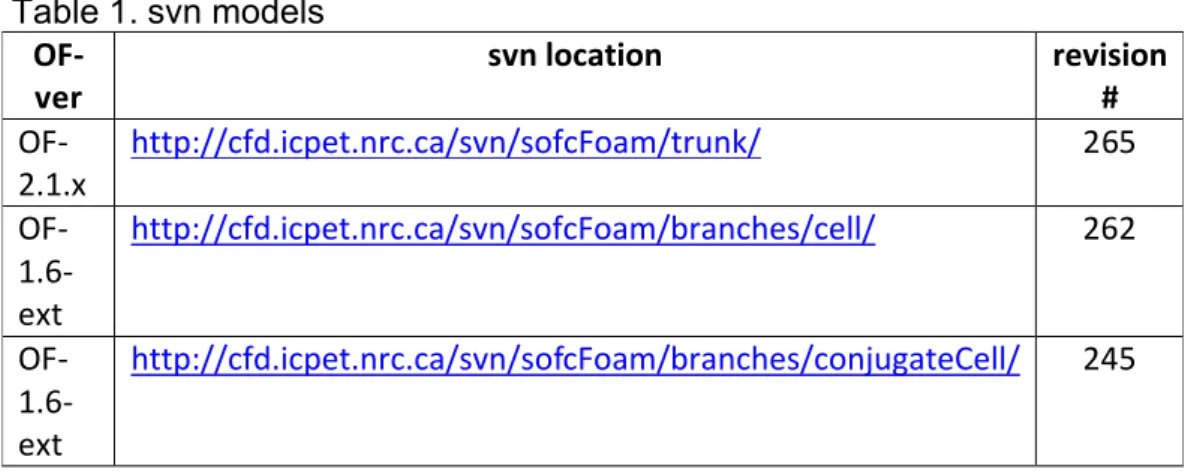
Table 1. svn models

OF-ver svn location revision #

OF-2.1.x http://cfd.icpet.nrc.ca/svn/sofcFoam/trunk/ 265 OF- 1.6-ext http://cfd.icpet.nrc.ca/svn/sofcFoam/branches/cell/ 262 OF- 1.6-ext http://cfd.icpet.nrc.ca/svn/sofcFoam/branches/conjugateCell/ 245

Revisions later than those shown in the table introduced run-time selection of species, first insofcFoam/branches/conjugateCell and then in sofcFoam/trunk. There is no further development planned forsofcFoam/branches/cell.

The latest version of the sofcFoam cell model can be downloaded from http://cfd.icpet.nrc.ca/svn/sofcFoam/trunk. Using the svn command line tool, one simply types

svn co http://cfd.icpet.nrc.ca/svn/sofcFoam/trunk at the prompt.

For a specific revision number, one modifies the above command as svn co –r <n> http://cfd.icpet.nrc.ca/svn/sofcFoam/trunk/

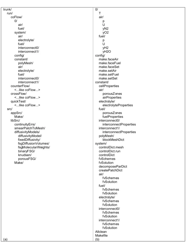
where <n> is the desired revision number, eg 265. The check-out delivers the directory structure shown in Figure 2(a) to the current working directory. Note that some of the file details change after the introduction of run-time selection of species. For those details, see the document gettingStarted_Cell268_OF21x.pdf at http://cfd.icpet.nrc.ca/svn/sofcFoam/trunk/docs/.

2.7 Directories

From Figure 2(a), the left panel of Figure 2, we see that the trunk/ directory has two main subdirectories, run/ and src/. The run/directory contains examples of cases that can be simulated with the cell model, while the src/directory contains the model source code. We examine both of these more closely, beginning with the src/ directory.

2.7.1 trunk/src/

The src/ directory contains the major subdirectories libSrc/ and appSrc/. In libSrc/, we find C++ classes that have been specifically developed or modified for

sofcFoam and are used in the cell model. The appSrc/ directory contains the cell model source files, which instantiate objects from both libSrc/ and OpenFoam/src as needed, to implement the cell model algorithm. As is typical for OpenFoam applications, the cell model application is built by including blocks of code (*.H files) into a main program (*.C file).

2.7.2 trunk/run/

The run directory contains case directories, or cases. The cases coFlow, counterFlow, and crossFlowexercise the model on co-flow, counter-flow, and cross-flow configurations, respectively. The case quickTest is similar to the coFlow case, but reduced from twelve to three channels. In each configuration, the fuel velocity is in the +x direction, while the air velocity is in the direction of +x, -x, and +y for co-flow, counter-flow and cross-flow, respectively.

Like any other OpenFoam case directory, the three cases here contain major subdirectories 0/, constant/, and system/. With only a single mesh, these 0/, constant/ and system/ directories would be populated by files only, but with multiple meshes they have a subdirectory for each region, and the files for each domain are placed in the appropriate directory or subdirectory. Thus initial global temperature T is found in 0/T, initial air velocity U in 0/air/U, initial fuel pressure p in 0/fuel/p, etc. Similarly, global cell properties are found in constant/cellProperties, whereas air properties are found in constant/air/airProperties. See Figure 2(b) for more complete listings.

trunk/ run/ coFlow/ 0/ air/ fuel/ system/ air/ electrolyte/ fuel/ interconnect0/ interconnect1/ config/ constant/ polyMesh/ air/ electrolyte/ fuel/ interconnect0/ interconnect1/ counterFlow/ <...like coFlow...> crossFlow/ <...like coFlow...> quickTest/ <...like coFlow...> src/ appSrc/ Make/ libSrc/ continuityErrs/ smearPatchToMesh/ diffusivityModels/ diffusivityModel/ fixedDiffusivity/ fsgDiffusionVolumes/ fsgMolecularWeights/ binaryFSG/ knudsen/ porousFSG/ Make/ (a) 0/ T air/ p U yN2 yO2 fuel/ p U yH2 yH2O config/ make.faceAir make.faceFuel make.faceSet make.setAir make.setFuel make.setSet constant/ cellProperties air/ porousZones airProperties electrolyte/ electrolyteProperties fuel/ porousZones fuelProperties interconnect0/ interconnectProperties interconnect1/ interconnectProperties polyMesh/ blockMeshDict system/ controlDict.mesh controlDict.run controlDict fvSchemes fvSolution decomposeParDict createPatchDict air/ fvSchemes fvSolution fuel/ fvSchemes fvSolution electrolyte/ fvSchemes fvSolution interconnect0/ fvSchemes fvSolution interconnect1/ fvSchemes fvSolution Allclean Makefile (b)

Figure 2. (a), left panel, directory structure from svn check out. (b), right panel,

2.8 Installation

In your chosen parent directory for the sofcFoam cell model, e.g. your

OpenFoam work space $WM_PROJECT_USER_DIR/applications/, check out the trunk/ directory from the Subversion repository. This creates directory trunkin the current working directory.

2.8.1 src

To compile the library and application source code, go to trunk/src/directory and run the Allwmake script. This should generate shared object library

libsofcFoam.so in the $FOAM_USER_LIBBINdirectory and application executable sofcFoam in the $FOAM_USER_APPBINdirectory. A lnInclude/ directory,

containing links to all of the libsSrc class files, will appear in the libSrc/ directory. 2.8.2 cases

As can be seen in Figure 2(b), a case directory contains only one polyMesh/ directory immediately after checkout, and it contains only the dictionary file blockMeshDict. This dictionary, together with the setSet batch command files in the <case>/config/ directory, describes the global and regional meshes. After the global mesh is made by the OpenFOAM utility blockMesh, the utility

splitMeshRegions generates the required regional meshes and map files. For more information on the blockMesh, setSet, and setsToZones utilities, see Chapter 5 “Mesh generation and conversion” and Section 3.6 “Standard utilities” in the OpenFOAM User Guide (http://www.openfoam.com/docs/user/).

Making the global and regional meshes is handled in sofcFoam/cell by the Makefile in the case directory. See, for example, run/coFlow/Makefile. The command

make mesh

will generate the global mesh and the region meshes. During model execution, various material property and other field values will be mapped from the region meshes to the global mesh. Cells that began life labeled as a fluid in the global mesh may have become a solid, and some of these may have boundary faces on the original fluid inlet or outlet patches. Accordingly, the fluid inlet and outlet patches may need to be redefined for the new reality. The redefinitions are specified by the make.face[Air|Fuel|Set]files in the configdirectory. See Appendix A for a description of the steps required to specify a new geometry.

2.9 Running the model

With the application already compiled, the command

will run the executable from the command line, using the available case data. The model can also be run by typing the executable name, and the output directed to Standard Out can be redirected to a file:

sofcFoam | tee log.run

Instead of running the model from the command line, a runscript is available to submit a job to a queue. The script usage line may need editing for your queuing system.

After the model has run to completion, VTK files for visualization, e.g. with paraview, can be prepared easily using the Makefile. Typing

make view

will generate VTK files for the last output step, whereas make viewAll

will generate VTK files for all output directories.

2.10 Mesh files

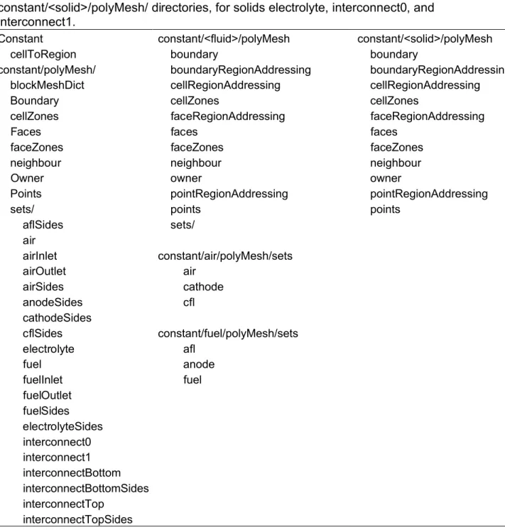
Before making the meshes the only mesh file is constant/polyMesh/blockMeshDict. Making the meshes introduces new directories and files as shown in Table 2 In addition to the standard boundary, faces, neighbour, ownerand pointsfiles, each domain has a cellZonesand a faceZonesfile. The original polyMesh directory, constant/polyMesh/, has a pointZones file and a sets/subdirectory containing cellSet information for each subregion and faceSet information for each patch. The regional polyMesh/ directories contain faceZonesand cellZones, as well as addressing files relating their domains to the global domain. The fluid regions, i.e., air and fuel, also have a sets/subdirectory, which contains cellSet

Table 2. Mesh files. Left: new files in constant, constant/polyMesh/ and

constant/polyMesh/sets after generating the meshes. Centre: files from meshing in the new constant/<fluid>/polyMesh/ directories, for fluids air and fuel, with additional file details for constant/air/polyMesh/sets/ and

constant/fuel/polyMesh/sets/ subdirectories. Right: files from meshing in the new constant/<solid>/polyMesh/ directories, for solids electrolyte, interconnect0, and interconnect1.

Constant constant/<fluid>/polyMesh constant/<solid>/polyMesh

cellToRegion boundary boundary

constant/polyMesh/ boundaryRegionAddressing boundaryRegionAddressing blockMeshDict cellRegionAddressing cellRegionAddressing

Boundary cellZones cellZones

cellZones faceRegionAddressing faceRegionAddressing

Faces faces faces

faceZones faceZones faceZones

neighbour neighbour neighbour

Owner owner owner

Points pointRegionAddressing pointRegionAddressing

sets/ points points

aflSides sets/ air airInlet constant/air/polyMesh/sets airOutlet air airSides cathode anodeSides cfl cathodeSides cflSides constant/fuel/polyMesh/sets electrolyte afl fuel anode fuelInlet fuel fuelOutlet fuelSides electrolyteSides interconnect0 interconnect1 interconnectBottom interconnectBottomSides interconnectTop interconnectTopSides

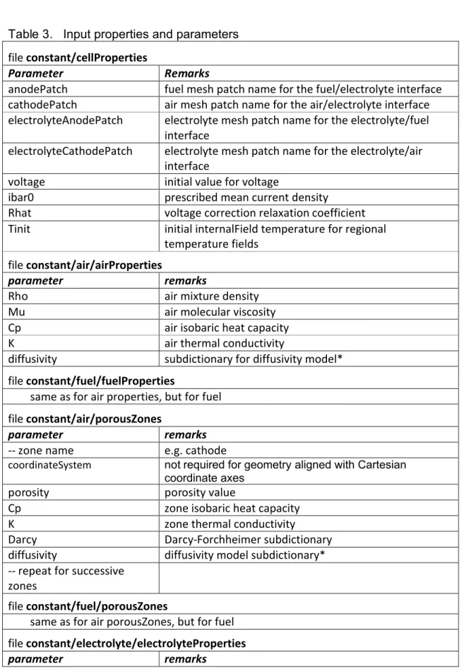
Table 3. Input properties and parameters file constant/cellProperties

Parameter Remarks

anodePatch fuel mesh patch name for the fuel/electrolyte interface cathodePatch air mesh patch name for the air/electrolyte interface electrolyteAnodePatch electrolyte mesh patch name for the electrolyte/fuel

interface

electrolyteCathodePatch electrolyte mesh patch name for the electrolyte/air interface

voltage initial value for voltage

ibar0 prescribed mean current density

Rhat voltage correction relaxation coefficient

Tinit initial internalField temperature for regional

temperature fields file constant/air/airProperties

parameter remarks

Rho air mixture density

Mu air molecular viscosity

Cp air isobaric heat capacity

K air thermal conductivity

diffusivity subdictionary for diffusivity model*

file constant/fuel/fuelProperties

same as for air properties, but for fuel file constant/air/porousZones

parameter remarks

-- zone name e.g. cathode

coordinateSystem not required for geometry aligned with Cartesian coordinate axes

porosity porosity value

Cp zone isobaric heat capacity

K zone thermal conductivity

Darcy Darcy-Forchheimer subdictionary

diffusivity diffusivity model subdictionary*

-- repeat for successive zones

file constant/fuel/porousZones

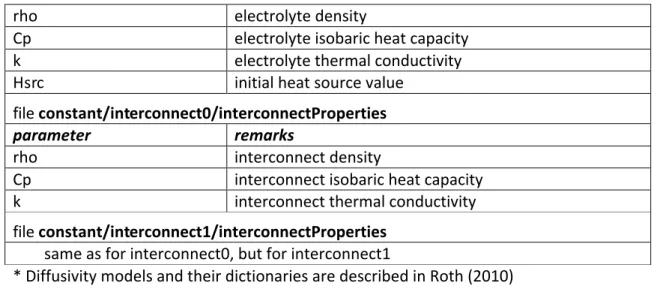
same as for air porousZones, but for fuel file constant/electrolyte/electrolyteProperties

rho electrolyte density

Cp electrolyte isobaric heat capacity

k electrolyte thermal conductivity

Hsrc initial heat source value

file constant/interconnect0/interconnectProperties

parameter remarks

rho interconnect density

Cp interconnect isobaric heat capacity

k interconnect thermal conductivity

file constant/interconnect1/interconnectProperties same as for interconnect0, but for interconnect1

* Diffusivity models and their dictionaries are described in Roth (2010)

Table 4. Input initial fields.

file physical field remarks

0/T cell temperature May be changed to suit operating conditions 0/k cell conductivity Inlet values = 0 prevents outward diffusion at inlets 0/air/p air pressure internalField and outlet boundaries at atmospheric

pressure

other patches zeroGradient or equivalent

0/air/U air velocity internalField 0 (or initialized to inlet value); inlet specified; outlet zeroGradient; cathodePatch type must allow code to set value (e.g. fixedValue) 0/air/yN2 mass fraction N2 internalField initialized to inlet value

cathodePatch must be type fixedGradient 0/air/yO2 mass fraction O2 as for yN2

0/air/diff gas diffusivity Inlet value = 0 prevents outward diffusion at inlet 0/fuel/p fuel pressure internalField and outlet boundaries at atmospheric

pressure

other patches zeroGradient or equivalent

0/fuel/U fuel velocity internalField 0 (or initialized to inlet value); inlet specified; outlet zeroGradient; anodePatch type must allow code to set value (e.g. fixedValue) 0/fuel/yH2 mass fraction H2 internalField initialized to inlet value

anodePatch must be type fixedGradient 0/fuel/yH2O mass fraction H2O as for yH2

2.11 Inputs

Runtime inputs to the model are supplied in dictionaries in the case directory. Among these are the mesh files and mesh mapping files generated during mesh generation, as discussed above. Tables 3 and 4 show the remaining fields and parameters that must be specified. The specifications supplied for the example coFlow/, counterFlow/, and crossFlow/cases can be viewed in their respective case files, as indicated by Table 3. Physical dimensions of all inputs are specified in the appropriate files as required by the OpenFOAM software. They are omitted in Tables 3 and 4.

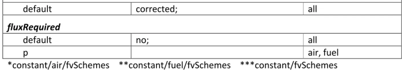
Numerical Schemes are specified at runtime by fvSchemesfiles in the system directories (system, system/air, etc). The fvSchemes dictionary contains a number of subdictionaries which must be defined for the code to run. In Table 5 we list the fvSchemes used by the model and the regions in which the listed schemes are applicable.

Table 5. fvSchemes settings

operator scheme applicable region(s)

ddtSchemes

default steadyState; all

gradSchemes

default Gauss linear; all

grad(p) Gauss linear; air*, fuel**

divSchemes

default none; all

div(rhoCpPhi,T) Gauss upwind; cell***

div(phi,U) Gauss GammaV 0.2; air, fuel div(phi,y) Gauss upwind; air, fuel

laplacianSchemes

default none; all laplacian(k,T) Gauss harmonic corrected; cell laplacian(mu,U) Gauss harmonic corrected; air, fuel laplacian((rho|A(U)),p) Gauss linear corrected; air, fuel laplacian(diff,y) Gauss harmonic corrected; air, fuel

interpolationSchemes

default harmonic; cell

default linear; fluid, solid regions

snGradSchemes

default corrected; all

fluxRequired

default no; all

p air, fuel

*constant/air/fvSchemes **constant/fuel/fvSchemes ***constant/fvSchemes Solver and other algorithmic controls and tolerances are supplied by the fvSolution dictionary files in the system directories, as shown in Table 6. Table 6. fvSolution settings

solvers dictionary

Field solver parameters region(s)

T PBiCG preconditioner DILU; tolerance 1e-10; relTol 0.0; maxIter 5000; cell p PCG preconditioner DIC; tolerance 1e-09; relTol 0; maxIter 700; air, fuel

U PBiCG preconditioner DILU;

tolerance 1e-09; relTol 0; maxIter 700; air, fuel yO2 yN2 yH2 yH2O

PBiCG preconditioner DILU; tolerance 1e-09; relTol 0.0; maxIter 700;

PISO dictionary air, fuel

parameter value nIteration nCorrectors nNonOrthogonalCorrectors pRefCell pRefValue 0 2 0 0 0 relaxationFactors dictionary field value p U yO2air 0.3 0.7 0.5 air, fuel air, fuel air

yN2air yH2fuel yH2Ofuel 0.5 0.1 0.5 air fuel fuel

Table 6 shows three subdictionaries in the fvSolution files: solvers, PISO, and relaxationFactors. In the solvers subdictionary, we find the settings for the linear solvers chosen to solve the discretized finite volume equations for the various fields. The relaxationFactors subdictionary contains under-relaxation factors to improve stability. The PISO subdictionary controls the PISO algorithm for the simultaneous solution of pressure and momentum. Table 6 also shows which regions (domains) use the tabulated settings. Note that the fvSolution file must exist in the system directory, even though it may not need any subdictionaries.

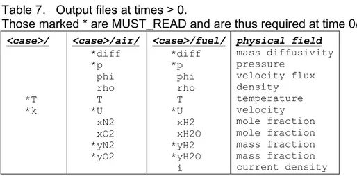
2.12 Outputs

The model writes selected fields to time directories in the case directory, and also writes to Standard Out as it proceeds.

2.12.1.1 Time directories

The model produces “time” directories in the case directory, in accordance with the settings in the control dictionary (system/controlDict). For a steady model like the cell model, these directory time names (e.g. 50/, 100/, etc.) represent

iteration count rather than time. Field IOobjects created with the AUTO_WRITE attribute will be written to these time directories. These include the MUST_READ fields present in the 0/ directories, and others, as shown in Table 7.

Table 7. Output files at times > 0.

Those marked * are MUST_READ and are thus required at time 0/

<case>/ <case>/air/ <case>/fuel/ physical field *T *k *diff *p phi rho T *U xN2 xO2 *yN2 *yO2 *diff *p phi rho T *U xH2 xH2O *yH2 *yH2O i mass diffusivity pressure velocity flux density temperature velocity mole fraction mole fraction mass fraction mass fraction current density

2.12.2 Run log

The model writes considerable information to Standard Out during each “time step”, of the iteration loop. Among these are residuals from linear system solvers, continuity errors, min, mean, and max of various fields, electrochemical information, etc.

2.13 Summary

Assuming you have OpenFOAM version 2.1.x with environment variables set, here is all you need to download, compile, and run the sofcFoam cell model. # obtain the code

cd <myChosenParentDirectory>

svn co http://cfd.icpet.nrc.ca/svn/sofcFoam/trunk/ cd trunk

# compile the model cd src

./ Allwmake

cd .. #return to trunk directory # generate meshes

cd run/<caseDirectory> #coFlow, counterFlow, crossFlow, ... make mesh

# run model from the command line with delivered settings make run

# generate VTK files for final output time make view

3. CASE STUDIES

Validation and verification (V&V) of the code is an ongoing activity that leads to confidence that the right calculations are being preformed, and that the

calculations are being performed right. In view of the limited experimental data both on fuel cell property values, and on detailed performance results, V&V was conducted by comparison of the OpenFOAM output with results from calculations with another CFD code, PHOENICS, under similar conditions, and also with simple spreadsheets for consistency of output and physical realism.

Subsequently several different geometries and operating conditions were considered in detail.

3.1 IEA geometry

The IEA geometry, Achenbach [14], was developed in the 1990s as a simple benchmark problem for code validation at the time. A journal paper on the subject has been submitted at the time of writing. In this paper, the present authors’ results are compared with those of the original IEA participants together with more recent work on the subject [15-17]. It was observed that the Reynolds and Péclet numbers for heat and mass transfer were less than unity for the fuel phase, and this has important implications on the problem formulation and computed results which fuel cell researchers (particularly those employing “black box” commercial codes) and non-CFD codes based on rate equation

formulations need to be aware of. Moreover some of the assumptions and

simplifications made in [14], such as the absence of porous diffusion layers, and limited chemical kinetics formulation suggest the IEA geometry is of limited use as a benchmark in the present day and age, although it is still useful as a first “reality check”.

3.2 Taiwan geometry

This geometry is based upon a somewhat idealized version of the Jülich F-design geometry. It is, however, more complex and physically realistic than the IEA case, above; the cell being composed of 9 layers: lower interconnect, air channel, cathode current collector layer, cathode functional layer, electrolyte, anode functional layer, anode substrate layer, fuel channel and top interconnect. It is idealized in that the manifolds are absent and the geometry of the design is somewhat simplified. This geometry formed the basis for the conference paper by Jeon et al. [18] which has now been submitted in a revised form as a journal paper [19] with the calculations being redone following a bug fix to the code. This journal article represents the first public disclosure of the MUSIC project at the cell level in archival form, including reference to the source code. Calculations

were performed for the cases of counter-flow, co-flow and cross-flow, and the results compared.

3.3 Jülich F-design

Figure 2. Computer aided design geometry used to generate computational grid for Jülich F-design

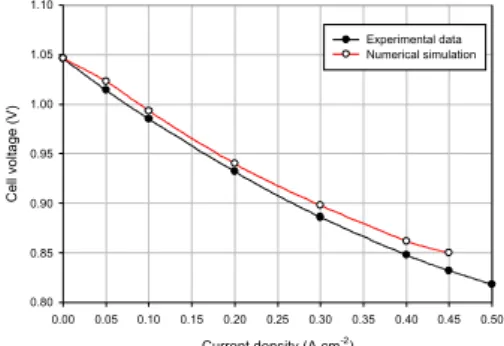
Figure 3. V-i performance curves, from ref. [20].

A conference paper with the first results for the Jülich F-design geometry [20] was presented. This is currently being expanded and improved to journal format. The F-design for stacks with anode supported cells (ASC) has been in use at Jülich since 2003, and significant experimental data is available. Cells are either 1010 cm2 _{or 2020 cm}2_{in size. The number of cells in the stacks tested to-date,} range from 2 up to 60. Figure 2 shows the CAD geometry used in construction of the computational mesh at NRC.

Anode supported cells with either double layer LSM cathodes or high

performance LSCF cathodes are generally used. Anode substrate and anode functional layers are both fabricated with conventional Nickel and Yttria-stabilised Zirconia (Ni/YSZ) cermet. The yttria stabilized zirconia (8YSZ) electrolyte layer is around 8 µm in thickness. A Gd-doped Ce-oxide layer is applied on the

electrolyte prior to depositing the LSCF cathode to prevent the inter-diffusion of cathode constituents into the zirconia electrolyte layer.

The interconnect plates, with integrated manifold structures for a counter-flow configuration of the reactants, are machined from e.g., Crofer22APU steel. A Ni-mesh is spot-welded to one side of the interconnect plate, providing a low resistance interface with the anode substrate. The Ni-mesh simultaneously acts as both a fuel gas distributor over the anode area and also provides electrical continuity. On the other side of the interconnect plates, channels are machined in the plates to distribute the air over the cathode surface. On the ribs between the channels a Mn-oxide layer and a perovskite type (LCC10) oxide layer are

deposited providing the low resistant interface with the cathode. For sealing, a glass-ceramic sealant from the BCAS-system is used. Table 8 lists the stack components and details for cells with LSCF cathodes, as used in kW-class,

Current density (A.cm-2₎

0.00 0.05 0.10 0.15 0.20 0.25 0.30 0.35 0.40 0.45 0.50 Cell voltage (V) 0.80 0.85 0.90 0.95 1.00 1.05 1.10 Experimental data Numerical simulation

F-design stacks. Material properties are given in Table 9.

Table 8.Components commonly used in F-design stacks

Stack / cell component Material Thickness

Interconnect / cell frame Crofer22APU 2.5 mm

Anode contact layer Ni-mesh 1.2 mm

Cathode contact layer perovskite type oxide

(LCC10) ~ 150 µm

Anode substrate Ni/8YSZ ~ 1500 µm

Anode functional layer Ni/8YSZ ~ 8 µm

Electrolyte 8YSZ ~ 8 µm

Diffusion barrier layer CGO ~ 5 µm

Cathode functional layer LSCF ~ 35 µm

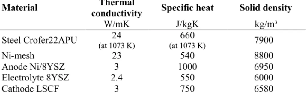
Table 9.Material properties of cell and stack components

Material _conductivityThermal Specific heat Solid density

W/mK J/kgK kg/m³

Steel Crofer22APU _{(at 1073 K)}24 _{(at 1073 K)}660 7900

Ni-mesh 23 540 8800

Anode Ni/8YSZ 3 1000 6950

Electrolyte 8YSZ 2.4 550 6000

Cathode LSCF 3 750 6580

The model is solved on six computational domains which together make up the fuel cell. These are air, fuel, electrolyte, middle plate, and two interconnects. All fields are specific to a domain; for example, air pressure and velocity are solved on the air domain, whereas hydrogen mass fraction is solved on the fuel domain. Each domain has its own temperature and thermal conductivity fields. The

temperature of the whole cell is computed by implicitly coupling temperature and thermal conductivities through adjacent boundaries, where it is required that both temperature and heat flux are continuous.

The computational domain of the F-design SOFC stack contains 65 parallel air channels with a Ni-mesh employed as the fuel distributor on the fuel side. A computational grid of over 3.4 million cells was used to tessellate the one-cell SOFC stack. The flow configuration is counter-flow. The motion of fuel and air in the porous anode and cathode regions are governed by Darcy’s law, which is implemented by introducing a distributed resistance as a volumetric source term in the momentum equation. Electrochemical reactions are treated as surface reactions occurring at the electrode-electrolyte boundaries. The resulting electrochemical mass fluxes provide boundary conditions for velocity and mass fraction on the air and fuel boundaries adjacent to the electrolyte. Gas inlet

velocities and temperatures are prescribed, with all other walls (apart from outlets) presumed adiabatic. Numerical convergence was identified when residual errors dropped below a reference tolerance.

Numerical calculations were performed under similar conditions to physical experiments, namely,_{i 0.3 A.cm}2_{with fuel/air utilizations of 15%/20%, inlet}

temperatures of 1023 K/973 K at 1.01325 bar. Figure 3 shows the V-i curve from the numerical model compared to that obtained from experiment. It can be seen that there is fair agreement between calculated and experimental data, with the former a little larger than the latter, especially at higher current density.

Figure 4. Air-side pressure Figure 5. Plate temperature

Figure 6. Air-side streamlines Figure 7. H2mass fraction

4. DISCUSSION OF RESULTS 4.1 Technical achievements

Working as a multi-disciplinary team with FZJ, FCRC, and Wikki, NRC led the development of multi-scale models for SOFCs using the open source software OpenFOAM. The technical work for the cell/small stack level model was mainly completed at NRC, whereas the micro-scale model was primarily built by FCRC. The cell/stack-level model is based on a Nernst potential minus losses

(overpotentials) algorithm with a complete CFD solution for flow and heat and mass transfer.

Two codes were developed:

(1) A “cell model” which consists of a parent mesh (for heat transfer) and several child meshes (fuel passages) for solving different variables (mass

fractions,velocities, pressures) and different equations (Navier Stokes, Darcy’s law etc.)

(2) A “conjugate model” where there is no parent mesh, only child meshes, obviating mesh decomposition. Avoiding mesh decomposition/splitting is a good idea/goal, but in practice we have to-date been obtaining the region meshes by splitting the parent mesh.

The model may readily be adapted for high temperature PEMs (FCRC are already doing this for another research programme)

The SOFC model was readily applied to (a) simple test cases developed at NRC (b) IEA benchmark case of Achenbach (c) Jülich simplified geometry, aka,

Taiwan geometry (d) Jülich Mark F geometry

The model accounts for variable density and specific heat as a function of composition and temperature, and different porous regions with effective diffusivities. Viscosity and thermal conductivity are however constants. In addition to the cell-scale model, a micro-model was successfully used to compute effective properties for porous media, based on numerically-generated packed spheres as well as tomography recontruction (FIB-SEM or X-ray). A prototype full two-potential model (for the electric fields) was also developed; and is currently being compared with existing Nernst-equation based model. A large-stack model is currently being worked-on by Nishida, Beale and Pharoah [8]. Three annual contracts (around $15K each) were given to Wikki to provide support and assist in program development. Monthly videoconferences, with minutes, were held to connect the researchers in Canada and Germany. The

working code and documentation is deposited in Subversion (SVN) repository at NRC, and is available for download by would-be users. A major advantage of developing MUSIC within OpenFOAM is that our code can be distributed freely to partners, clients and stakeholders. That is not true for commercial licensed

products

4.2 Problems encountered

The grid generation application(s) associated with OpenFOAM are of rather limited application compared to commercial GUI-based products. However we have successfully built grids for both the full F-design, and complex 3-phase micro-scale domains with the OpenFOAM snappyHexMesh code.

The fuel cell code itself does not have a proper GUI-based user interface and this would need to be carefully designed. A few bugs caused significant delays in the project. Code development was slower than expected. Specifically:

The mesh decomposition script in the conjugate code failed to reassign boundary faces on the parent mesh in accordance with the assignment of cells to the child meshes. A very long time was taken to identify and fix this problem.

Parallelization has proved to be an ongoing issue which has still not been entirely resolved.

Problems arose when different individuals made various changes to the same code and then checked them in, destroying other peoples’ work. Fortunately because the SVN repository was employed, there was a path back and these changes could be reconciled. While irritating, this did not cause a particularly long delay. However some protocol for code management, when multiple researchers are involved, needs to be established.

Documentation for OpenFOAM is far from extensive, and courses for programmers and students are quite expensive.

Although the user/programmer has the source code, this is of little use if he/she does not understand the program architecture, and this is difficult due to the hierarchical nature of object-oriented code, and inheritance of C++ class objects. Future investment in the use of more sophisticated/professional programming environments, such as the integrated development environment (IDE) Eclipse (http://www.eclipse.org/) is possibly warranted. However, it is often difficult to pursuade researchers and graduate students to work in a professional software engineering environment/mode.

http://www.wikki.co.uk/

(founded by one of the original OpenFOAM code developers) created version 1.6ext which differs significantly from v1.6 which was developed by OpenCFD. These companies are in a constant state-of-evolution and are dependent on being able to obtain contracts to survive. Thus software “forks” are inevitable. Open software is not free software, rather it is prudent to obtain some sort of funding arrangement with one or more of these companies in order to obtain timely solutions to problems if and when they arise.

4.3 Suggestions for future work

At present only hydrogen fuel has been considered with binary fuel and oxidant mixtures. In order to add, say, methane, or more general arbitrary fuel and oxidant combinations, with multiple chemical and multi-step electrochemical reactions etc., careful planning is required (NB: Work for generalized species is in fact in progress, but so far only for a single chemical reaction). The heat source terms also need to be split up (at present these only occur in the electrolyte).

The next logical step is the development of a community of users for the SOFC suite of codes. This could be undertaken by FZJ and/or NRC and/or FCRC in a stand-alone mode or under the auspices of an intergovernmental program such as the International Energy Agency. An example of an existing special interest group is the OpenFOAM working group on turbomachinery.

The development of a high-fidelity experimental data base of both property values and performance measures such as polarisation curves and temperature, species and local current density distributions is highly desirable.

Expansion of the repository to include multiple fuel cell types (SOFC, HT-PEMFC, DMFC) at multiple scales (micro, cell, small/large stack) in a manner consistent with existing OpenFOAM library cases is important. Mounting of the suite on an open source repository such as SourceForge.net would increase exposure to the worldwide community.

The code could further be adapted for application to other electrochemical processes and products, such as electrolysers and batteries, in due course.

5. CONCLUSIONS AND RECOMMENDATIONS

It was shown that the open source CFD code, OpenFOAM, could be successfully used to develop mathematical models of hydrogen fuel cells. Initial development was at the cell and small stack level, with subsequent focus on micro-scale and large stack-type models. The use of open source software obviates expensive annual license fees associated with commercial codes, and allows researchers complete access-to and control of the underlying models. Commercial CFD software products are generally geared towards industrial clients with well-defined products and processes, readily amenable to standard analysis. Fuel cells are an emerging product involving a significant research component for which the open source environment allows more control.

The advancement of OpenFOAM as a useful tool for practical applications relies on a measure of sponsorship by government agencies and/or academic

communities, worldwide. It would be advisable for the MUSIC community to procure a measure of support from one or more of the OpenFOAM

development/application houses in order that a well-balanced suite of software be maintained. As additional users start to use the MUSIC suite, this will become increasingly important. One particular area for concern is mesh generation where, at present, there is a deficit of open source codes able to meet the demanding requirements required for practical engineering fuel cells. This may be mitigated in the future as more users embrace the open source paradigm. The basic algorithm developed in the small stack/cell model described in this report and also the two potential models, section 1.5.3, may readily be adapted for HT-PEMFCs. Similarly, micro-scale models [9] would appear to be readily applicable with some modification. Large-scale SOFC stack models may prove less amenable for application to PEMFC stacks, if the membrane resistances associated with hydration in PEMs show substantial local variation in the through plane direction. This is a subject for further research.

APPENDIX I: SPECIFYING MESHES FOR A NEW GEOMETRY

Figure A1 shows the proposed geometry we intend to model. The associated dimensions of the components are given in Table A1. The vertical structure can be captured by seven blocks, as shown in Figure A2, (the block containing the electrolyte is too thin to be discernible). The blocks containing the air and fuel channels can then be split horizontally to separate the channels from the ribs, the latter being part of the interconnects.

Figure A1. A fuel cell with one air channel and one fuel channel. Left panel shows air (blue) and fuel (purple) inlets, interconnects (grey) and electrode sides. Centre panel shows air (blue) and fuel (purple) volume regions, each comprised of both a channel and a porous electrode zone. Right panel shows lower (blue) and upper (red) interconnect regions.

Table A1. Dimensions and extents of the cell components.

interconnect0 channelair cathode electrolyte anode channelfuel interconnect1

xlow 0 0 0 0 0 0 0

length [mm] 50 50 50 50 50 50 50 ylow 0 1 0 0 0 1 0 yhigh 4 3 4 4 4 3 4 width [mm] 4 2 4 4 4 2 4 zlow 0 3.5 5.00 5.29 5.3 6.3 6.3 zhigh 5 5.0 5.29 5.30 6.3 7.8 11.3 height [mm] 5 1.5 0.29 0.01 1 1.5 5

Figure A2. Vertical block structure. Bottom to top: interconnect0, air, cathode, electrolyte (too thin to discern), anode, fuel, and interconnect1.

We begin with a blockMeshDict dictionary that will create a parent mesh

consisting of the seven vertical blocks (Figure A2), which for convenience, going from bottom to top, we refer to as interconnect0, air, cathode, electrolyte, anode, fuel, and interconnect1. Although the geometry shows symmetry about the y = 2 plane, we construct the entire domain for illustrative purposes. Here is the list of points for the blockMeshDict file:

blockMeshDict

convertToMeters 0.001; vertices

(

// ... From Bottom To Top // Interconnect0 ( 0 0 0) // 0 (50 0 0) // 1 (50 4 0) // 2 ( 0 4 0) // 3 // Interconnect0_to_Air ( 0 0 3.5) // 4 (50 0 3.5) // 5 (50 4 3.5) // 6 ( 0 4 3.5) // 7 // Air_to_cathode ( 0 0 5.0) // 8 (50 0 5.0) // 9 (50 4 5.0) //10 ( 0 4 5.0) //11