Boosting sparse representations for image retrieval

Boosting Sparse Representations for Image Retrieval

by

Kinh H. Tieu

Submitted to the Department of Electrical Engineering and Computer Science

in partial fulfillment of the requirements for the degree of

Master of Science in Computer Science and Engineering

at the

MASSACHUSETTS INSTITUTE OF TECHNOLOGY

February 2000

@

Massachusetts Institute of Technology 2000. All rights reserved.

A uthor... ..

. . . .. . . . .. . . . .

Department of Electrical Engineering and Computer Science

January 31, 2000

j /'?

Certified by...

. . . . .. . . .. .. . .. .. . .. .. . . .. . .. . .. . .. .. . .. . .. .. . .. ..

Paul Viola

Associate Professor, Department of Electrical Engineering and Computer Science

Thesis Supervisor

Accepted by ...

...

Arthur C. Smith

MASSACHUSETTS INSTITUTE OF TECHNOLOGY

MAR 0 4 2000

LIBRARIES

Chairman, Department Committee on Graduate Students

,,I Z1,

MiTLibraries

Document Services

Room 14-0551 77 Massachusetts Avenue Cambridge, MA 02139 Ph: 617.253.2800 Email: docs@mit.edu http://libraries.mit.edu/docs

DISCLAIMER OF QUALITY

Due to the condition of the original material, there are unavoidable

flaws in this reproduction. We have made every effort possible to

provide you with the best copy available. If you are dissatisfied with

this product and find it unusable, please contact Document Services as

soon as possible.

Thank you.

Boosting Sparse Representations for Image Retrieval

by

Kinh H. Tieu

Submitted to the Department of Electrical Engineering and Computer Science on January 31, 2000, in partial fulfillment of the

requirements for the degree of

Master of Science in Computer Science and Engineering

Abstract

In this thesis, we developed and implemented a method for creating sparse representations of real images for image retrieval. Feature selection occurs both offline by choosing highly selective features and online via "boosting". A tree of repeated filtering with simple kernels is used to compute the initial set of features. A lower dimensional representation is then found by selecting the most selective of these features. At query time, boosting selects a few of the features useful for the particular query and ranks the images in the database by taking the weighted vote of an ensemble of classifiers each using a single feature. This method allows for a large number of potential queries and facilitates fast retrieval on very large image databases. The method is tested on various image sets using standard measures of retrieval performance. An online demo of the system is available via the World Wide Web1.

Thesis Supervisor: Paul Viola

Title: Associate Professor, Department of Electrical Engineering and Computer Science

Acknowledgments

This research was supported in part by Nippon Telegraph and Telephone.

First I thank this great nation for giving me and my family hope. My life would be drastically different without the incredible opportunities I have received here.

Thanks to the Massachusetts Institute of Technology and the Artificial Intelligence Laboratory for supporting my studies and providing superb resources for my research.

I thank all the members of the Al Lab that have helped me along the way, especially the Learning

and Vision Group. Special thanks to John Winn, Dan Snow, Mike Ross, Nick Matsakis, Jeremy De Bonet, Christian Shelton, John Fisher, Chris Stauffer. Extra special thanks to Erik Miller for reading the thesis and offering helpful comments.

Thanks to Professor Eric Grimson for advice, support and helping me to fulfill my academic requirements in a timely and worthwhile manner.

Finally, I thank my advisor Professor Paul Viola for his care, encouragement, support, and insight. He has greatly enriched my understanding of this work and of how to do research. It is a rewarding and pleasurable experience working with Paul, and I appreciate the time, energy, and thought that he provides.

For my family, I would not be here without your unconditional encouragement, support, and love.

Contents

1 Introduction

1.1 Thesis Summary . . . . 1.2 Image Retrieval . . . .

1.2.1 The Problem Model . . . .

1.2.2 Specifications . . . . 1.3 Scene Analysis . . . . 1.4 Image Indexing . . . . 1.4.1 Measurement Space . . . . 1.4.2 Similarity Function . . . . 1.5 Selective Measurements . . . . 1.5.1 Image Generation . . . . 1.5.2 Measurement Design . . . . 1.6 Learning a Query . . . . 1.7 Performance Evaluation . . . . 1.8 Im pact . . . .

1.9 Why Try to Solve Image Retrieval Today? . . .

1.10 Thesis Organization . . . .

2 Previous Approaches

2.1 Color Indexing . . . . 2.1.1 Histograms . . . . 2.1.2 Correlograms . . . . 2.2 Color, Shape, Texture . . . .

2.2.1 Q B IC . . . . 2.2.2 CANDID . . . . 2.2.3 BlobWorld . . . . 2.2.4 Photobook . . . . 2.2.5 JACOB . . . . 2.2.6 CONIVAS . . . . 2.3 W avelets . . . . 2.4 Templates . . . . 2.4.1 VisualSEEk . . . . 2.4.2 Flexible Templates . . . . 2.4.3 Multiple Instance Learning and Diverse

2.5 Database Management Systems . . . . 2.5.1 Chabot . . . .

2.5.2 SCORE . . . .

2.6 Summary of Previous Approaches . . . .

2.7 Related Work . . . .

2.7.1 Information Retrieval . . . .

2.7.2 Object Recognition . . . .

2.7.3 Segmentation . . . .

2.7.4 Line Drawing Interpretation . .3 3 Selective Measurements 36 3.1 Motivation . . . . 36 3.1.1 Preprocessing vs. Postprocessing . . . . 36 3.1.2 Image Representations . . . . 37 3.1.3 Sparse Representations . . . . 38 3.2 D esign . . . . 38 3.2.1 F ilters . . . . 39 3.2.2 Filtering Tree . . . . 40 3.2.3 Color Space . . . . 41 3.2.4 Normalization . . . . 42 3.3 Measurement Selection . . . . 42 3.3.1 Selectivity . . . . 42

4 Learning Queries Online 44 4.1 Image Retrieval as a Classification Task . . . . 44

4.2 Aggregating W eak Learners . . . . 45

4.3 Boosting Weak Learners . . . . 45

4.4 Learning a Query . . . . 46

4.5 Observations . . . . 46

4.6 Relevance Feedback . . . . 48

4.6.1 Eliminating Initial False Negatives . . . . 49

4.6.2 Margin Boosting by Querying the User . . . . 49

5 Experimental Results 50 5.1 Performance Measures . . . . 50

5.2 Natural Scene Classification . . . . 50

5.3 Principal Components Analysis . . . . 52

5.4 Retrieval. . . . . 52 5.5 Face Detection . . . . 52 5.6 Digit Classification . . . . 53 6 Discussion 64 6.1 Summary . . . . 64 6.2 Applications . . . . 64 6.3 Research Areas . . . . 65 6.4 Connections to Biology. . . . . 65 6.5 Future Research . . . . 65

A Implementation of the Image Retrieval System 67 A.1 Architecture . . . . 67

A.2 User Interface . . . . 67

A.3 Online Demo . . . . 67

5 . . . 35

List of Figures

1-1 An airplane and a race car may be classified as belonging to the class of vehicles using

functional property "transportation" . . . . . 11

1-2 Example images from an airplanes and a race cars class defined by visual properties. 11 1-3 Schematic of an image retrieval system. . . . . 13

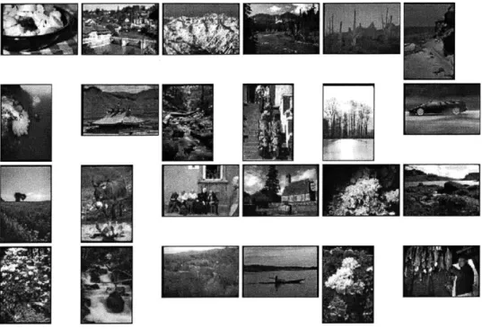
1-4 A set of random images (that can be found on the World Wide Web) that illustrates the diversity of visual content in images. . . . . 14

1-5 An example of a scene with many objects and complex relationships between the

objects. For example, is the Golden Gate Bridge the only important object in the image? Are the mountains in the background important? Should it be classified as a scene of a coastline? Are the people in the foreground important? There are many ways to describe this image, the difficulty lies in being able to represent all these relationships in a tractable manner . . . . 15 1-6 A query on the AltaVista system (which uses color histogram measurements) for

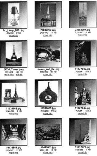
images similar to the sunset image in the upper left corner. Here color is effective because orange colors dominate in images of sunsets but not in other images. . . . . 17 1-7 A query on the AltaVista system for images similar to the image of the Eiffel Tower

in the upper left corner. Color is ineffective for a queries such as this one where background colors (i.e., the blue sky here) dominate. . . . . 18 1-8 Possible renderings of two images generated by picking a few specific itmes from a

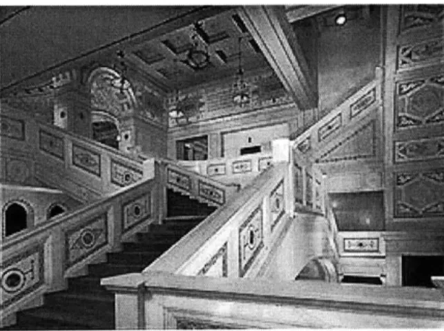
large dictionary of visual events. . . . . 19 1-9 The diagonal pattern of vertical edges (marked in red) arising from the stairs in this

image represent a "staircase" pattern. . . . . 20

1-10 The boosting process iteratively constructs a set of classifiers and combines them into

a single boosted classifier. . . . . 21

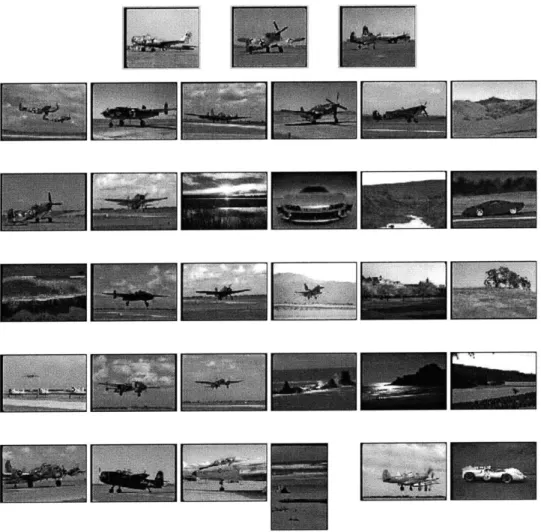
1-11 A query on the system described in this thesis for images similar to the three example

images of airplanes at the top. . . . . 22 2-1 The color histograms for both images are very similar because they both contain

similar amounts of "yellow"," green",and "brown". However most people would agree that these images represent very different visual concepts. . . . . 25

2-2 A hand-crafted template for images of waterfall scenes. Here the waterfall concept is defined to be a white region in between two green regions with a blue region on top. 30 2-3 An E-R diagram for an image of a sailboat. . . . . 31

2-4 A query on the AltaVista system with the keyword "Eiffel" that illustrates the rich semantic content of particular words. Since an image would probably be labeled "Eiffel" only if it contained an image of the Eiffel Tower, text is effective for this query. 33

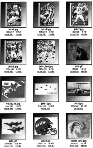
2-5 A query on the AltaVista system with the keyword "jets". Although we wanted

images of jet propulsion vehicles, the system retrieved images of the Jets football team. 34

3-1 The image on the right is a permutation of the pixels of the image on the car (left). Using too general an image representation allows for these kinds of unrealistic images. 37

3-2 On the left are the principal components of image patches. On the right are the

principal components of the responses to the fourth principal component on the left

(a bar-like filter). . . . . 39

3-3 The 9 primitive filters used in computing the measurement maps. In practice, these can be efficiently computed with separable horizontal and vertical convolutions. . . . 40

3-4 A schematic of the filtering tree where a set of filters is repeatedly applied to an image to capture more global structure. . . . . 41

3-5 Response of an image of a tiger to a particular filtering sequence. Note that this feature has detected a strong peak corresponding to the arrangement of the stripes on the body of the tiger... ... 42

3-6 Histograms for a highly selective (left) and unselective measurement (right). The highly selective distribution had a selectivity of 0.9521 and a kurtosis of 132.0166. The unselective measurement had a selectivity of 0.4504 and a kurtosis of 2.3703. . . 43

4-1 Some typical images exhibiting the "waterfalls" concept. Note the diversity in the images as some contain sky, some contain flora while others are mostly rock, etc. . . 44

4-2 The left plot shows how boosting finds measurements which better separate images of mountains from other images better than choosing random measurements (right). 48 4-3 The boosting measurements which separate well images of mountains do not discrim-inant im ages of lakes as well. . . . . 48

4-4 At left is the initial performance. On the right is the improved performance after the most four most egregious false positives were added as negative examples. This example is on a data set containing five classes with 100 images in each class (see C hapter 5). . . . . 49

5-1 An example image from each class of sunsets, mountains, lakes, waterfalls, and fields. 51 5-2 Measurements with four layers of filtering (right) performed better than using only one layer of filtering (left). . . . . 51

5-3 A comparison between using color histograms with the chi-square similarity function (left) and using selective measurements and boosting (right). . . . . 52

5-4 Here we show that boosting can be used with color histograms to give comparable performance. Boosting achieves this using only half of the histogram measurements. This results in a substantial computational savings on a large database. . . . . 53

5-5 A query for waterfalls using color histograms and the chi-square function. Note global color histograms cannot capture the flowing vertical shape of waterfalls. . . . . 54

5-6 A query for sports cars using color histograms and the chi-square function. Note unsurprisingly that the few cars found are all red-cars of other colors in the database are not ranked highly. . . . . 55

5-7 A query for waterfalls using color histograms and boosting. Note that boosting finds images with similar color distributions, but most of those images are not of waterfalls. 56 5-8 A query for sports cars using color histograms and boosting. Note that boosting finds images with similar color distributions, but most of those images are not of cars. . . 57

5-9 The principal components correlations (left) are much smaller than the original mea-surem ent correlations (right). . . . . 57

5-10 Performance is reduce using the principal components of the measurements. . . . . . 58

5-11 A query for sunsets. The positive examples are shown on the left. . . . . 58

5-12 A query for waterfalls. The positive examples are shown on the left. . . . . 59

5-13 A query for sports cars. The positive examples are shown on the left . . . . 60

5-14 A query for cacti. The positive examples are shown on the left. . . . . 61

5-15 The average receiver operating curve (left) and precision-recall curve (right) for de-tecting faces. . . . . 61

5-16 A query for faces. The positive examples are shown on the left. . . . . 62

5-17 Results for images of the ten digits. . . . . 62

5-18 Results for images of the ten digits. . . . . 63

6-1 An image with various possible classifications based on visual content, context, prior

know ledge, etc. . . . . 66 A-1 Image retrieval system architecture. . . . . 67 A-2 Image retrieval interface. . . . . 68

List of Tables

2.1 A comparison of different image retrieval systems. . . . . 32

4.1 The boosting algorithm for learning a query online. T hypotheses are constructed each using a single feature. The final hypothesis is a linear combination of the T

hypotheses where the weights are inversely proportional to the training errors. . . . 47

Chapter 1

Introduction

1.1

Thesis Summary

Today, with digital cameras and inexpensive mass storage devices, digitizing and storing images is easier than ever. It is not uncommon to find databases with over 500,000 images [33]. Moreover, multimedia content on the Internet continues to grow dramatically-in 1995, there were an estimated

30 million images on the World Wide Web [47], today that number is certainly much higher. This explosion of images creates a need to be able to index these databases so that users can easily and quickly find particular images. The goal of an image retrieval system is to provide querying capabilities comparable to those which exist for text document databases such as [2]. The problem involves designing an image representation suitable for retrieval and an algorithm for learning a query. The representation must somehow capture the visual content in images. Since the images desired are not known ahead of time, it is difficult to provide the learning algorithm with many training examples. So training often occurs with only the few training examples provided by the user. A further requirement of the entire system is that it must operate in real time so that it can be used interactively.

This thesis presents an approach to the image retrieval problem that is motivated by the statistics of real images (i.e., images of real scenes, not computer generated ones). The task is: "Given some description of visual content, find images which fit the description." In other words, given a concept or class of images, find other images exhibiting the same concept or belonging to the same class. This has important implications for computer vision because being able to find images which match an arbitrary description implies being able to concretely describe an image. In other words, there must be an explicit description of every image so that the description can be compared (by a computer) to the target concept.

Humans can retrieve images easily and almost unconsciously especially because we can compare the functional properties of objects in an image. For example both the airplane and race car in Figure 1-1 could be assigned to a "vehicle" class since both provide transportation. This type of categorization may be regarded as "higher" level cognition and resembles [39]'s superordinate categories. Functional categorization requires more than just visual features of an image; some characterization of the function "transportation" is needed. This type of characterization may also involve some assessment of the utility of objects. Strategies for using functional properties are not well developed, even in more constrained domains such as text document retrieval. It is exactly the ease and mystery with which our brains perform this task that makes it extremely difficult to program a computer (which currently requires explicit instructions) to do it'. We will sidestep this problem by only considering information which can be extracted from the "visual content" of images. For example, although our system should be able to identify the Eiffel Tower as a tower, it is not expected to infer meta properties such as "(location Paris)". Thus, it is reasonable to expect our system to be able to categorize airplanes as one class, and race cars as another, since each of those

Figure 1-1: An airplane and a race car may functional property "transportation".

be classified as belonging to the class of vehicles using

Figure 1-2: Example images from an airplanes and a race cars class defined by visual properties. classes share many visual characteristics as shown in Figure 1-2. This formulation of the problem is commonly known as "query by image content". This more closely corresponds to the "basic level" categorization of [39]. We can thus formulate image retrieval as the following task:

Given very few example images, rapidly learn to retrieve other examples.

For over 20 years, computer vision has tried to develop systems which take an arbitrary input image and generate a scene description. This general problem has been decomposed into more specific subproblems such as image segmentation, object detection and object recognition. The idea is that if we could solve the subproblems and combine the results, we could compute a complete description of an image and hence compare images by comparing descriptions. Although progress has been made in each of the subproblems, each remains unsolved. Part of the reason for this is that the subproblems are intimately related in subtle ways since having a perfect segmentation would help isolate areas in an image for detection or recognition, and having a perfection detection or recognition system would help us find the segmented regions corresponding to different objects. Research in fusing the results of these subsystems is less developed.

We will attack the image retrieval problem without trying to explicitly solve the computer vision subproblems. This reasoning is motivated by the observation that one should not try to solve a more difficult intermediate problem if one can more easily solve the problem directly [49]. We will exploit

the statistics of real images by presuming that although many possible events (i.e., visual events such as an image of the Eiffel Tower) may occur in an image, in any particular image, only a small set of events will actually happen. This observation suggests a sparse distributed representation for images. We will design a set of features such that for any particular image, only a few key ones will be active. However over all possible images, each feature should have about equal probability of being active. These features will necessarily be selective, meaning the average response over all images is much lower than the strong responses for a few particular images. To measure the similarity between images, a system can learn which are the important features and compare just those features.

To select the most relevant subset of features with only a few example images, "boosting" [20] is used create a series of learners. Each successive learner tries to do better on examples that the previous one did poorly on. This approach is well suited to image retrieval since the selective features can be computed offline once and for all. The learning can be performed quickly with just a few training examples because the representation is sparse. Since only a few relevant features will be selected, the entire database of images can be searched with fewer computations per image.

Besides being a possible solution for image retrieval, this thesis suggests a theory for useful generic intermediate level image representations suitable for simple, fast learning with a small number of training examples.

1.2

Image Retrieval

1.2.1 The Problem Model

Image retrieval can be decomposed into two parts as shown in Figure 1-3: image indexing storing images in a representation that facilitates retrieval.

querying learning the deserved query concept, and searching the database for images matching the concept.

Image indices are typically precomputed offline so that they do not have to be recomputed for each query. Depending on the type of index used, this may limit the kinds of queries which are possible, but improves retrieval speed. For example if only color information is stored in an index, then queries based on shape will not be possible. However for queries involving color, only the index is required, and the image never needs to be rescanned. Querying is typically performed online as this is part of the interactive user interface of the retrieval system.

In machine learning, a concept is induced or "learned" given a set of training examples. The concept could be a rule to discriminate between images of airplanes and race cars. Machine learning is often applied to classification problems where the problem is to assign a label given an input. The training examples are usually given as a large set of labeled data (x", tn) where X" is the

nth

input image and t' is the corresponding target label. The goal is to learn the concept so that unseen test examples can be labeled correctly. Traditional machine learning methods for classification are difficult to apply to retrieval because they often require a small number of known classes and many labeled training examples. Retrieval differs from classification because the target class is unknown in advance, and only defined at query time. In addition, it is possible for a single image to be relevant for two different queries (e.g., an image picturing a sailboat off the coast of France may be relevant both for a query of boats and coasts). Making matters worse, image databases are often huge (thousands or millions of images) and usually contain a diverse set of images as shown in Figure 1-4.

Formally, the task is to rank all the images in a database according to how similar they are to a query concept using a ranking function:

r(x, Q) : x -* [0,1] (1.1)

where x is an image to be ranked,

Q

= q1,. .. qN are example images of the query concept, 0 stands

user-selected examples

learn query concept

retrieved results

Figure 1-3: Schematic of an image retrieval system.

inde imae

=

image database

representation

I

4com-m,

Figure 1-4: A set of random images (that can be found on the World Wide Web) that illustrates the diversity of visual content in images.

Q.

Typically N ranges from 1-5. This situation calls for a way to index the images in the database to allow for fast (because online users will not tolerate a long response delay) and flexible (because different users will want to retrieve different types of images) machine learning of r(x,

Q)

using very few training examples.

1.2.2

Specifications

Image retrieval is a difficult problem because it is not clear how to best represent images. For text, because words have such rich semantic content, significant results have been achieved by merely considering documents as lists of word counts without any regard for word order. An image retrieval system must also be efficient in order for it to be practical on large databases. Below are the two primary requirements of an image retrieval system:

fast search through a large database (thousands or millions of images) quickly (milliseconds or

seconds).

flexible handle a large number (hundreds or thousands) of different image queries (concepts) such

as sunsets, cars, crowds of people, etc.

As noted in [46], an image retrieval system must operate in real time. This allows the system to make use of relevance feedback from the online user. Feedback generally consists of the user choosing more examples and eliminating unwanted ones.

The method of specifying queries determines the type of user interface an image retrieval system should have. We have chosen an interface where a query is specified by choosing a set of example images representative of the class of images implied by the query. This is commonly known as "query

by example". It frees the user from having to manually draw an image or from trying to describe

the visual content with words 2. In particular a system should not demand too much of the user except for a few simple tasks such as:

Figure 1-5: An example of a scene with many objects and complex relationships between the objects. For example, is the Golden Gate Bridge the only important object in the image? Are the mountains in the background important? Should it be classified as a scene of a coastline? Are the people in the foreground important? There are many ways to describe this image, the difficulty lies in being able to represent all these relationships in a tractable manner.

browsing cycling through random images.

positives choosing some positive examples of the desired concept.

negatives possibly choosing some negative examples.

feedback possibly doing a few rounds of relevance feedback. corresponding to picking more positives

and negatives.

1.3

Scene Analysis

Based on the formulation of the image indexing problem, it seems appropriate to represent each image as a description of the scene that was imaged. This description would include the various objects in the image and how they are related spatially and by other relations. To determine the similarity of two images, we simply determine the similarity of the scene descriptions. There are several reasons that this type of system does not exist today. First, there does not exist a robust method for extracting scene descriptions given an image. To do that we must first be able recognize arbitrary objects in an image. Object recognition is an ongoing goal of computer vision and continues to defy a general solution. Second, it is not clear what should be considered an object (i.e., should the mountains in Figure 1-5 be recognized as one object or multiple mountains?). Finally given two scene descriptions, it is not clear how similarity should be measured. Do we find how many objects images x and y have in common, or are the spatial and other relationships between the objects more important?

1.4

Image Indexing

The first step to creating an image retrieval system is to develop a representation for images that facilitates retrieval. Image indexing takes an input image (initially represented as an array of pixel intensities) and produces a new representation that makes it easy to find a particular set of images in a database. One way to think of this problem is to consider the analogous task of making indices for books in a library. For example, a book might be indexed by author, title, publication date, as well as by an abstract. The goal of the index or representation is to permit quick access of a particular book or class of books.

1.4.1

Measurement Space

To index images, we need to take some measurements from the input image. Let us define a measurement as some function of the original pixel values of the image. Assume that we have some way of extracting a set of measurements M from an input image. For example, one measurement could be the count of the number of pixels of a certain color. Assuming the elements xi of M are scalars (i.e., xi C R), we can arrange them into a measurement vector x = [x1, .. . , Xd]T where d is the

total number of measurements. We can thus consider an image as an element of the abstract space

Rd.

This is the multidimensional input (usually called a "feature" vector, although that connotes binary measurements) commonly assumed by many classical pattern recognition techniques [18].

1.4.2

Similarity Function

We can define the similarity s(x, y) between two images (vectors) x and y simply as a function of the L2 distance between the vectors:

s(x, y) = e-d(xY)2 (1.2)

where

d

d(x, Iy) = (Xi - yi)2 (1.3)

i1

is the L2 distance. Points x and y are maximally similar if they are represented as the same point

in

Rd

since the L2 distance between them will be 0 and their similarity with be the maximum value

of 1 (note that d(x, y) > 0). As the distance between two images in measurement space linearly increases, the similarity will decrease exponentially. This formulation is equivalent to saying that similarity is proportional to the density of x under a spherical gaussian centered on y (or vice versa) since s(-, -) is in the form of a gaussian density:

A~X) = 1/ e-(XI)T E'(X-L). (1.4)

V/2 |r I |,1/2

Note that the similarity function is probably not the correct or "natural" metric for images in measurement space. For example, the triangle inequality property of the distance functions may not be valid (e.g., red is similar to orange and orange is similar to yellow, but the sum of these two distances can be smaller than the distance between red and yellow since these colors may appear very dissimilar). In addition, it is unclear whether or not similarity should decrease exponentially with distance.

Based on sample query results, many commercial image retrieval systems today appear to use color histograms (pixel color counts as measurements) and a static ranking function such as:

r(x, Q) s(x, Y) (1.5) where N n = E q (1.6) n= 1

is the sample mean of the measurements of the example images. Once again, this is equivalent to similarity being proportional to the density of the gaussian centered at p. In these systems, first a color histogram representation would be generated for every image in the database. A user specifies a query by choosing an example image. The system then retrieves the most similar images by finding the images which are closest to the example image in the L2 sense. Color histograms work well when

M 33 6 KU

more into skririb more into sia!nil

more into SM&

moe in I&J

7MUM3 25 KB

mom inlo Jbik

mote Wo LO

moreinto j~jlj m2 Ludo lft

Figure 1-6: A query on the AltaVista system (which uses color histogram measurements) for images similar to the sunset image in the upper left corner. Here color is effective because orange colors dominate in images of sunsets but not in other images.

such as sunsets as shown in Figure 1-6. However as shown in Figure 1-7, color is inadequate for a query of images of the Eiffel Tower. In fact the system has done a better job of finding blue sky than tall, steel framed structures. Even with useful measurements, using a single static similarity function may not be appropriate for every type of query. For example, although blue sky was not an important feature for the Eiffel Tower query, it may be useful in queries for airplanes.

1.5

Selective Measurements

1.5.1

Image Generation

Consider the following observation of real images:

Many possible visual events can occur in images, but in any particular image, only a few

will actually happen.

Suppose we want to generate some image. We can pick from a very large "dictionary" of visual events (e.g., clear or cloudy sky, grassy, sandy, or rocky ground, a dalmatian, a sports car, the Taj Majal, etc.). For example we can generate an image of a sports car on the beach. In the background would be the ocean and perhaps some waves and a few mossy rocks. We could have generated an entirely different picture such as one of grazing buffalos. Possible renderings of these images are shown in Figure 1-8. Note however that we cannot have too many things in any single image-it

more nmo sip

ODMN= 44 KB

rnore iAO Itik

72m72 I KB

Z95x4S3 59 KB 45x3Z5 W KB more inbo snrrb more rdo sinflr more -nio smiira

Dnx358 lS KB 31x23 18KB 177xZ57 2n KB more inbo stniar more inbo simiik more inbo smirB

2sox370 127 KB 2x23 46 KB 12sx92 2 KB more ino s'mibr moreinbo snhibr more irno sinr

4m6xo312 13 Kb

more inio s milaf

Figure 1-7: A query on the AltaVista system for images similar to the image of the Eiffel Tower in the upper left corner. Color is ineffective for a queries such as this one where background colors

Figure 1-8: Possible renderings of two images generated by picking a few specific itmes from a large dictionary of visual events.

is very unlikely to have both the buffalos and sports car in the same scene. The statistics of real images allows for many types of images but not too many types of visual events in one particular image (e.g., we are very unlikely to find an image of an aircraft carrier and a herd of camels on the slopes of Mt. Everest).

Now suppose we want to know how similar image x and y are. Since we hypothesize that images are generated by selecting visual events, one reasonable approach is to determine the similarity between the events in x and y. So if both x and y contain a sports car on the beach, we might say x is very similar to y. Of course, remember that we are given images in the form of arrays of pixel intensities. Since there is no explicit representation of visual events, we will try to make measurements which respond when these events are present. It is as if we must somehow explain how an image is produced from the abstract generative model of images previously described. The key question is how to design our measurements.

1.5.2

Measurement Design

Our approach is based on extracting "selective measurements" of images which correspond to the visual events that we are interested in. Intuitively these are relatively global, high level structural organizations of more primitive measurements. A primitive measurement such as an edge can occur in many places in a particular image3. We are more concerned with higher order events such as a specific pattern of edges as in tiger or zebra stripes or a "staircase" pattern. Figure 1-9 shows how a diagonal arrangement of vertical edges correspond to a staircase pattern. We believe that a key characteristic of these events is that they are sparse. Measurement for these events will be selective since they will only respond when a group of pixels are arranged in a specific pattern. A measurement which detects whether a pixel is green or not will not be selective since many pixels of an image may be green and furthermore many images will contain green pixels.

We have designed a filtering sequence that attempts to extract selective measurements. The first stage of filtering uses masks which signal primitive events such as oriented edges and bars. Each successive stage of filtering uses the same set of filters but of increasing support (the ratio of the filter and image sizes) and is applied to the response images of the previous stage. The idea is to capture the structural organization of lower level responses.

Note that by itself, the ability to uniquely identify every image is not useful. In fact the array of pixels representation is already adequate for that purpose. However it does not suggest an obvious way to generalize (i.e., grouping a set of images as members of a class). We can view this most primitive representation as "overfitting" particular images. In machine learning, a classifer is a system which when given an input outputs the corresponding class label. Just as we can trivially build a classifier with zero training error by simply memorizing the training samples with a lookup

3

Figure 1-9: The diagonal pattern of vertical edges (marked in red) arising from the stairs in this image represent a "staircase" pattern.

table, we can just as easily assign a unique label (e.g., 1, 2, ... , N) to each sample. However it is

unlikely that two images will ever have the exact same array of pixel values, so this method will not allow us to label new images. For example, a slight translation of all the pixels to the right will cause a change in almost every one of the array values. However, we would still regard the slighted shifted image as very similar to the original image. We need measurements which occur at an intermediate level of representation. This will enable our system to compare these measurements and use them to identify a variety of image classes. We have designed our selective measurements to fill this need. An added benefit of selective measurements is that they can speed up learning. Selective measurements will induce a sparse representation for images. In other words, only a few measurements will be active for a particular class of images. Thus a learning algorithm need only focus on those particular measurements useful for identifying images in the class.

1.6

Learning a Query

To take advantage of the selective measurements representation of images, we will use a "boosting" framework to learn the concept implied in a class of images. In our case we would like a classifer which will tell us whether an image belongs to say the class of waterfall images (i.e., is similar to a set of example images of waterfalls). Often it is quite easy to construct a classifer which performs better than chance simply by using some sort of information in the image such as whether or not there exists a striped pattern. Using other measurements we can build more weak classifiers which perform better than random, but not much better. Boosting [20] is a general method for improving a weak classifier by iteratively constructing a set of them and linearly combining their outputs into a single boosted classification. Since only a few key measurements will be meaningful for a particular image class, the goal of the learning algorithm is to find these key measurements. Boosting starts

by constructing a classifier which uses only one measurement. It then modifies the distribution of

training example images so that incorrectly classified ones are more heavily weighted. The process is then repeated by selecting another measurement and building a second classifier. After a few iterations, we have a set of classifiers, each of which is like a rule of thumb for classifying an image. Boosting ensures that when all the classifiers are linearly combined, the weighted classification is more accurate. Figure 1-10 shows a schematic of the boosting process.

Boosting takes advantage of the learning algorithm's ability to adapt to different training data and explicitly reweights specific training examples to alter the distribution of the training data. Boosting enables the learning algorithm to select the key measurements most relevant for the given query and ignores the rest. After this initial training phase, querying the entire database only requires

select a new measurement

-* classifier I

-build classifier classifer 2 boosted_classifier

14

classifer M P

--test classifier

adjust weights weights

Figure 1-10: The boosting process iteratively constructs a set of classifiers and combines them into a single boosted classifier.

computations with T measurements, where T is the number of boosting iterations. Empirically we have found that 10 to 50 measurements gives reasonable results. As a practical advantage, this makes storing the image representations in an inverted file more efficient. An inverted file indexes the database by measurement instead of by image. For example file 1 contains measurement 1 for all images, file 2 contains measurement 2 for all images, etc. This type of organization is more useful for the boosting procedure which looks at one measurement in multiple images at a time.

1.7

Performance Evaluation

It is difficult to evaluate image retrieval performance because ground truth does not exist. Intuitively we all know how a good system should perform, but there does not exist an image database such that for any given query, the optimal results are well defined. The enormity of databases and the multitude of possible queries make constructing a standard test database difficult. Ultimately, the best measure is correlation with human judgments of similarity. Figure 1-11 shows an example query of the image retrieval system using selective measurements and boosting. Many people would agree that most of the retrieved images are similar to the example images. We will carefully construct some test databases and evaluate performance using standard measures borrowed from information retrieval [26].

1.8

Impact

In addition to being a practical tool for image indexing, search, and categorization, an image retrieval system must necessarily address important theoretical questions in vision and learning. The task of looking for images similar to an example image implies a definition of similarity for images. This definition in turn relies on an understanding of how to represent and explain images. Humans can retrieve images with ease. By formalizing this problem and developing a system to solve it, we can gain insight into the brain's solution. Note that the different types of possible queries (or concepts) is very large. The image retrieval system must be general enough to measure similarity for very different types of images, ranging from images of sunsets to crowds of people. Although developing measurement detectors for eyes, noses, and mouths will enable queries for faces or people, they will not work for queries of cars, waterfalls, etc. It is difficult to know how many image concepts need to be supported. In addition, the desired image class remains unknown until a query is specified. What

I measurements

Figure 1-11: A query on the system described in images of airplanes at the top.

this calls for is a set of measurements that is general enough for a large class of images. The problem with using many different measurements is that learning structure in large measurement spaces is more difficult. This problem is exacerbated by the fact that we can only expect users to provide a few example images of the class. Many traditional machine learning techniques require hundreds or thousands of examples to learn a concept. Thus the image retrieval problem is a practical need, and presents important challenges to computer vision and machine learning.

1.9

Why Try to Solve Image Retrieval Today?

Our approach to image retrieval describes images with visual content measurements. Finding the measurements themselves is a difficult problem and currently most representations use undiscrim-inating measurements such as color histograms. In addition, learning the query with only a few example images is a difficult task. Despite these shortcomings the advantage of this approach is that it deals with visual content directly making the system more intuitive and natural. It also allows for an investigation into the statistics of real images and learning with only a few examples. Thus instead of waiting for a complete general theory of vision to be found or remaining content with text annotation for images, our exploration with image retrieval may yield some interesting results and point out other problems that need to be solved.

1.10

Thesis Organization

In this introduction we provided the reader with an overview of the image retrieval problem and proposed an approach motivated by the statistics of real images. We also briefly introduced ideas in computer vision, machine learning, and information retrieval which are relevant to this research. The rest of the thesis details the ideas presented here.

Chapter 2 surveys the current approaches to image retrieval. Both historical approaches and current state of the art methods will be examined. We will compare our approach to previous methods and point out where our primary contribution lies. We will also briefly mention related work.

Chapter 3 begins the discussion of the approach to the problem. We describe a method of ex-tracting selective measurements from images and selecting particular measurements for the retrieval task.

In Chapter 4, we describe how the image representation developed in Chapter 3 is used for image retrieval. We will present the approach for learning image concepts with very little training data.

In Chapter 5, we will show the results of experiments using our approach for image retrieval. We also discuss our method of selecting and using image data sets and various performance measures.

Chapter 6 summarizes our work and discusses future research directions.

Chapter 2

Previous Approaches

Approaches to image retrieval have been primarily exploratory. There is no satisfactory theory for why certain measurements and classifiers should be used. Although there has been an explo-sive growth of digital image acquisition and storage technology, researchers have only begun to improve image retrieval technology. These systems can be divided into feature/measurement based approaches such as [46, 23, 6, 29, 38, 19, 43, 25, 10, 1, 34, 24] and database management system approaches such as [33, 3]. Some common characteristics of many previous approaches are:

* Only a single positive example is used. " Negative examples are often not considered.

" The user is required to adjust the weights (importance) of various features. " The user often needs to be experienced with an intricate query language.

* Various features are used without a principled way of combining them. * There is no query learning, only a fixed similarity function.

These characteristics put a heavy burden on the user to be familiar with the intricacies of the retrieval system. Often a particular example image and set of weights will work well, but a slightly different setting of the weights or a different example will drastically alter the retrieval. Many of the early systems were tested on very small databases (on the order of a hundred images). This is a small number compared to the typical size of current image collections, and a miniscule fraction of the number of images on the World Wide Web.

2.1

Color Indexing

2.1.1 Histograms

One of the earliest approaches to image indexing used color histograms [46]. A color space such as RGB (red, green, blue) is discretized into a fixed set of colors c₁, ... , cd to be used as the bins of the histogram. The color histogram for an image is simply a table of the counts of the number of pixels in each color bin. [46] used the following "histogram intersection" similarity function:

s(x, t) = Z min(xi, ti) (2.1)

zi=1

ti

where x is the test image, t is the model image, and i indexes the bins in the histogram. This gives the sum of the fractional matches between the test image and the model. If objects in x and t are segmented from the background, then this is equivalent to the L, distance (sum of absolute values) of the histograms treated as Euclidean vectors. Color histograms work well for a database with a

Figure 2-1: The color histograms for both images are very similar because they both contain similar amounts of "yellow"," green",and "brown". However most people would agree that these images represent very different visual concepts.

known set of segmented objects which are distinguishable by color (i.e., the magnitude of the color variation of the object under different photometric conditions is within the color quantization size).

The advantages of color histograms that motivate their use are:

" Histograms are easy to compute (in

O(N)

time using

O(d)

space where N is the number of

pixels).

* They are invariant to translation and rotation in the image plane, and to pixel resolution. * Color is a much simpler and more consistent descriptor of deformable objects (e.g., a cloud, a

sweater) than rigid shape-based representations.

The disadvantage of histograms is that we lose information about the distribution of color or shape of colored regions. This is because the histogram is global and no attempt is made to cap-ture any spatial information. By definition, the histogram can be computed by treating all pixels independently, since color is a pixel level property. These extremely local measurements are then combined into global counts. The implicit assumption is that the spatial distribution of color is unimportant. However the simple example in Figure 2-1 shows that this is not the case. Two other assumptions are: (1) all colors are equally important, (2) colors in the same discrete color bin (uni-formly discretized) are similar. [46] performed experiments in which the model image was assumed to be segmented so that the histograms were not corrupted by noisy backgrounds. They used a small database of 66 images of objects well differentiated by color (e.g., different cereal boxes and shirts). For a practical system, users would be required to segment objects in the model image. This would require that the histograms be computed online, slowing down the overall retrieval process. Note that no attempt was made to use multiple examples and negative examples. Also there was no machine learning of queries. Although there are an exponential number of possible histograms (in the number of colors m), for real images, this space is effectively much smaller because some combinations of colors are highly unlikely. Also many dissimilar objects such as red cars and red apples will be tightly clustered, while similar objects such as red cars and black cars will be distantly separated in the color histogram space. So color histograms naturally only work well when the query is adequately described by global counts of colors, and these counts are unique to images relevant to the query.

2.1.2

Correlograms

Color correlograms augment global color histograms to describe the spatial distributions of colors

[23]. The correlogram of an image is the set of pairwise distance relationships between colors:

9ci,cjk(x) = Pr [p2 E cc,|p1 - p21 = k]. (2.2)

pi Eci,P2

It gives the probability that any pixel pi colored ci is within an L,, distance (i.e., maximum vertical or horizontal distance) k from any pixel P2 colored cj. Note that the correlogram is still global

in a way because it describes how a particular color ci is distributed across the image. It is a generalization of the simple color histogram because we can always get the pixel color counts by marginalizing the "auto correlogram" gc,c ,k over all distances k. To keep the correlograms small and tractable, in practice k ranges discretely from a set D such as {1, 3, 5, 7} (i.e., the assumption is that large spatial correlations are not useful for similarity). In this way, color correlograms can be computed in O(M 2NIDI) time (without any optimizations) where IDI is the cardinality of D. [23] also augmented the simple L1 distance by considering a "relative" L1 distance where the degree

of difference in a bin is inversely proportional to the average size of the bin counts (to account for

Weber's Law 1):

d(x, t) =

Z

j','k(X) -- i,,k ( . (2.3)

ij.k gci,cj,k (t) + 9ci,cj,k (X) + 1

[23] demonstrated reasonable retrieval results on experiments where a scene was imaged

un-der different photometric conditions and unun-derwent small transformations such as translation and rotation. Since color is fairly stable under different lightning conditions and translation and rota-tion, correlograms work well for retrieving images of the same scene. However for general queries of different scenes which are similar (e.g., images of cars of different colors), color alone is not a discriminative enough measurement as previously discussed.

2.2

Color, Shape, Texture

2.2.1

QBIC

QBIC (Query By Image Content) [19] is a highly integrated image retrieval system that incorporates many types of features/measurements. Queries may be specified with an example image or by a sketch. Text annotations can be used as well. QBIC can also process video sequences by breaking them into representative frames and using the still image tools to process each frame. Users define a query using average color, color histograms, shape, and texture (although these can only be selected from a predefined set of sample textures). Users are also required to weight the relative importance of these features. Shape is described by first doing a foreground/background analysis to extract objects. Then edge boundaries of the object are found. Comparing shapes is fairly expensive even though QBIC uses dynamic programming [12]. In addition, histogram similarity is measured using a quadratic distance function

d(x, y)= (X y)TA(x - y) (2.4)

where the matrix A specifies some notion of similarity between pairs of colors. A few prefiltering schemes are used to attempt to speed up retrieval since computing a quadratic distance can be slow. Although QBIC offers a slew of features, they are not much more discriminative than those used by color indexing approaches. Users must also be intimately acquainted with the system to properly weight the relative importance of features.

2.2.2

CANDID

CANDID (Comparison Algorithm for Navigating Digital Image Databases) [25] attempts to prob-abilistically model the distribution of color, shape, and texture in an image. At each pixel in an image, localized color, shape, texture features are computed. A mixture of gaussians probability density is used to describe the spatial distribution of these features in the image. A mixture density

'Results from psychophysics experiments on sensory discrimination show that for a wide range of values, the ratio of the "just noticeable difference" to the stimulus intensity is constant [27].

is

M

p(x) = Zp(xj)P(j) (2.5)

j=1

where P(j) is the prior probability of x being generated from gaussian j. In particular P(j) must satisfy

E,

P(j) = 1. The parameters for the mixture model are estimated using the K-means

clustering algorithm [8]. The similarity of two images I, and 12 is measured using a normalized inner product similarity function

f1

P11 (x)PI2 (x)dx

nsi(R = P2) (2.6)1

[fP (x) dx fR PI2(xd]/

which is the cosine of the angle between the two distribution functions. The mixture of gaussians model avoids the need to arbitrarily designate discrete bins when using histograms. It does require choosing in advance the number of components or clusters M. An added advantage of modeling the distribution is that it is possible to visualize the relative contribution of individual pixels to the overall similarity score. [25] achieved good results on restricted databases of satellite and pulmonary

CT scan images with 100 and 200 total images respectively. The primary disadvantage of CANDID

is that both the density estimation and querying phases are relatively slow and will not scale well to larger databases.

2.2.3

BlobWorld

In the BlobWorld [6] system, images are represented as a set of "blobs" or 2D ellipses of arbitrary eccentricity, orientation, and size. Blobs are constrained to be approximately homogeneous in color and texture. This representation is designed to reduce the dimensionality of the input image while retaining discriminatory information (i.e., the assumption that homogeneous blobs are adequate for discrimination). By using blobs of coherent color instead of global color histograms, some local spa-tial information is preserved. In this respect, blobs are similar to correlograms with small distances. Texture is measured by the moment matrix of the horizontal and vertical image gradients, and a ''polarity" term which measures the extent to which the gradients agree.

To cluster points under the color and texture dimensions the expectation-maximization (EM) algorithm [8] is used to fit a mixture of gaussians model. The algorithm iteratively tries to find the parameters for each gaussian such that the log likelihood of the data under the parameters is maximized. The number of clusters chosen ranges from two to five, and is selected based on the minimum number of clusters which fit the data adequately (this means using one fewer cluster if the log likelihood does not drop too much). In effect, this clustering determines a discrete set of prototype colors and textures. After clusters are found, a majority voting and connected components algorithm is used to group pixels into blobs. EM is then used again to find the two dominant colors and mean texture within a blob. The spatial centroid and scatter of the blob is also computed.

To formulate a query, the user first submits an image. The system returns the blob representation of the image. The user then chooses some blobs to match and weights their relative importance. Each blob is ranked using a diagonal Mahalanobis distance, and the total score is combined using fuzzy logic operations on the blob matches.

[6] shows experiments in which BlobWorld outperforms the simple color histogram approach of

[46].

2.2.4

Photobook

The philosophy of Photobook [34] is to index images in a way that preserves enough information to reconstruct the original image. To achieve this, the system is divided into three separate subsystems. The first subsystem attempts to capture the overall "appearance" of the image. This is done using principal components analysis [48]. This method describes an image by the deviation from an average