Human body shape prediction and analysis using predictive clustering tree

Publisher’s version / Version de l'éditeur:

2011 International Conference on 3D Imaging, Modeling, Processing,

Visualization and Transmission (3DIMPVT), pp. 196-203, 2011-07-18

READ THESE TERMS AND CONDITIONS CAREFULLY BEFORE USING THIS WEBSITE.

https://nrc-publications.canada.ca/eng/copyright

Vous avez des questions? Nous pouvons vous aider. Pour communiquer directement avec un auteur, consultez la première page de la revue dans laquelle son article a été publié afin de trouver ses coordonnées. Si vous n’arrivez pas à les repérer, communiquez avec nous à PublicationsArchive-ArchivesPublications@nrc-cnrc.gc.ca.

Questions? Contact the NRC Publications Archive team at

PublicationsArchive-ArchivesPublications@nrc-cnrc.gc.ca. If you wish to email the authors directly, please see the first page of the publication for their contact information.

NRC Publications Archive

Archives des publications du CNRC

This publication could be one of several versions: author’s original, accepted manuscript or the publisher’s version. / La version de cette publication peut être l’une des suivantes : la version prépublication de l’auteur, la version acceptée du manuscrit ou la version de l’éditeur.

For the publisher’s version, please access the DOI link below./ Pour consulter la version de l’éditeur, utilisez le lien DOI ci-dessous.

https://doi.org/10.1109/3DIMPVT.2011.32

Access and use of this website and the material on it are subject to the Terms and Conditions set forth at

Human body shape prediction and analysis using predictive clustering

tree

Xi, Pengcheng; Guo, Hongyu; Shu, Chang

https://publications-cnrc.canada.ca/fra/droits

L’accès à ce site Web et l’utilisation de son contenu sont assujettis aux conditions présentées dans le site LISEZ CES CONDITIONS ATTENTIVEMENT AVANT D’UTILISER CE SITE WEB.

NRC Publications Record / Notice d'Archives des publications de CNRC:

Human Body Shape Prediction and Analysis Using Predictive Clustering Tree

Pengcheng Xi, Hongyu Guo, Chang Shu

Institute for Information Technology National Research Council Canada

Ottawa, Ontario, Canada

{Pengcheng.Xi, Hongyu.Guo, Chang.Shu}@nrc-cnrc.gc.ca

Abstract—Predictive modeling aims at constructing models that predict a target property of an object based on its descriptions. In digital human modeling, it can be applied to predicting human body shape from images, measurements, or descriptive features. While images and measurements can be converted to numerical values, it is difficult to assign numerical values to descriptive features and therefore regression based methods cannot be applied. In this work, we propose to use Predictive Clustering Trees (PCT) to predict human body shapes from demographic information. We build PCTs using a dataset of demographic attributes and body shape descriptors. We demonstrate empirically that the PCT-based method has similar predicting power as the numerical approaches using body measurements. The PCTs also reveal interesting struc-tures of the training dataset and provide interpretations of the body shape variations from the perspective of the demographic attributes.

Keywords-Predictive modeling; digital human modeling; pre-dictive clustering tree; demographic attributes;

I. INTRODUCTION

Many applications require realistic 3D models of human shape. One way of doing this is through digitizing real humans using 3D imaging techniques like range scanning. Indeed, large databases of range scans have been collected to form samples of entire populations. The scans can be further processed to build statistical models in which the variability of human shape can be analyzed. The statistical models allow parameterizing the space of human shape and thus generate an arbitrary number of virtual, but statistically real human shapes.

A statistical model of the human shape can also be used as priors to infer 3D shapes from partial shape information. For example, Blanz and Vetter [7] use a statistical model, called

morphable model, built from 3D scans of faces to reconstruct 3D face models from 2D images. 3D body shapes can also be generated from traditional anthropometric measurements such as height, waist circumferences, and the lengths of the limbs [2].

In practice, demographic data are also collected in 3D anthropometry surveys. For example, in the CAESAR survey (CAESAR - Civilian American and European Surface An-thropometry Resource), information such as age, ethnicity, marital status, occupation, etc. are collected [14]. Many of these attributes are non-numerical. For example, marital

status may have values like “single”, “married”, “divorced” or “widowed”. Intuitively, some of these attributes must relate to body shape. Natural questions arise: can we pre-dict human body shape from some of these demographic attributes? If so, to what extent can we predict? The answers to these questions have potential applications in many areas. For example, in a forensic investigation where a suspect’s picture is not available, face or body shape may be predicted from other features, e.g., age, ethnicity, marital status and occupation. One may also use this kind of prediction for designing and marketing products for targeted populations. In this paper, we predict human body shapes from descrip-tive features. We propose to exploit the relationship between human body shape and demographic information using Predictive Clustering Trees (PCTs) [8]. PCTs capture the structure of the data by building hierarchical clusters. Once the PCTs are constructed from the training data, prediction is done by traversing the trees using the descriptive attributes. Besides shape prediction, the PCTs also provide induction rules that help us analyze the shape data from the perspective of the descriptive attributes.

We test the proposed approach on the CAESAR database which consists of 5,000 full-body scans sampled from the North American and European populations. Each scan is accompanied with 44 traditional anthropometric measure-ments and 19 demographic attributes. We compare our approach using the demographic data with the prediction using numerical anthropometric measurements as it is done by Allen et al. [2]. Our experiments show that the PCT-based approach has similar predictive power.

The contributions of this work consist of two parts:

• 3D body shape prediction from demographic attributes. This is particularly useful when body measurements are not available.

• an interpretation of body shape difference with respect to demographic attributes.

II. RELATEDWORK

Much work has been done on the statistical shape analysis of human heads [7], [11], [20] and bodies [1], [4], [5], [18]. Parameterization of raw scans creates new representations which are consistent on head or body features. This enables a morphable shape model being built for training-based

applications, which include reconstruction from measure-ments [1], [2], [15], 2D images [6], [7], [9], [16], [19], landmarks [1], [4], and partial scans [3], [4].

Allen et al. [1] introduce a consistent parameterization approach by fitting a generic body model to each body scan, and thus build a morphable shape model. This model can be used for feature analysis by learning a linear mapping from body measurements to Principal Component Analysis (PCA) coordinates [2].

Blanz and Vetter [7] apply a morphable face model to reconstructing face models from sample images by fitting a 3D morphable model to 2D images. Facial attributes, such as gender, attractiveness and expressions are controllable through modifying parameters. Similar to this approach, Seo et al. [16] suggest a data-driven approach to reconstructing human body shape from the silhouettes.

Anguelov et al. [4] introduces a pose deformation model and a shape model for shape completion to partial view completion and motion capture animation. Amberg et al. [3] introduces an expression-invariant method for face recogni-tion by fitting an identity/expression separated 3D morphable model to shape data.

A common character in the above approaches is that the input can be converted to numerical values. For example, contours extracted from an input image are represented by coordinates of sampled 2D points. These approaches may fail if descriptive features become part or all of the input. In this work, we introduce data mining techniques that are suitable for handling nonnumeric inputs.

Blockeel et al. [8] introduce an approach which adapts the basic top-down induction of decision trees towards clus-tering. It employs the principles of instance based learning. According to Langley [13], each node of the tree corre-sponds to a concept or a cluster, and the tree as a whole thus represents a kind of taxonomy or a hierarchy.

A Predictive Clustering Tree (PCT) introduced by Dze-roski et al. [12] allows for predicting multiple target vari-ables. Human body shape in a statistical shape space can be represented by multiple variables like PCA coordinates. Therefore, it is naturally applicable to predicting body shapes from descriptive features.

III. STATISTICAL MODEL

In CAESAR database, every raw scan of human body contains about150, 000 vertices and 300, 000 triangles. For shape correspondence (also called consistent shape param-eterization), we implemented a template-based approach as that of [18]. For data compression, we performed PCA on the parameterized shape data. A shape space is thus built with the following steps.

1) Represent each parameterized shape as a vector xi,

i = 1, ..., m1(m1 is the number of subjects used for

building a shape space), and arrange all the vectors into a matrix X = (x1, x2, ..., xm₁). A covariance

matrix cov(X) =P (xi− x)(xi− x) T

is calculated, where x is the mean vector of all the xi.

2) We next perform eigen-decomposition of the covari-ance matrix. It creates a series of eigen vectors Φj

and their corresponding eigen values λj, where j =

1, ..., (m1− 1). The eigen values are in a descending

order.

3) Since all the Φj are orthogonal to each other, they

form the bases of the shape space. Organizing Φj in

columns forms a new matrixΦ. Each shape vector xi

can be mapped into this space through

Bi= ΦT(xi− x) (1)

which is comprised of mapped coordinates along the principal components. It is thus a new representation of the original 3D shape vector.

4) If a vector of coordinates bj is given, a new shape

xnew can be reconstructed through:

xnew= x + m₂

X

j=1

Φjbj (2)

where m2(< m1) is the number of principal

compo-nents to be used for reconstruction. IV. PREDICTIVE CLUSTERING TREE

Predictive clustering is a general framework that combines clustering and prediction [8]. It partitions a dataset into clusters so that variations in each cluster are minimal and those between clusters are maximal. It is similar to clustering but differs in that predictive clustering builds a predictive model (an induction rule) to each cluster.

Predictive clustering tree constructs a model for predicting a multi-objective target based on its description. The model is learned from a set of examples for building a decision tree. They have the form (D, T ), where D means descriptions and T denotes the target object. At each node, the PCT tries to find the best partition rule using D through minimizing the variations of clustered T . As a result, each leaf node represents a cluster, and the conjunction of the conditions on the path from the root to the leaf forms the induction rule [12].

A. Example for building a PCT

As an example, we look at a hypothetical weather predic-tion problem. We build a PCT using a small set of training data [17] listed in Table I, where weather outlook and wind conditions are input D and temperature and humidity are output T .

Building a PCT amounts to trying different partition tests and computing the in-cluster and between-cluster variations. In this example, the first test is trying “Outlook = sunny” and putting testing cases into one cluster if the condition is met and those into another cluster otherwise. Following this partition is to calculate the in-cluster and between-cluster

Outlook Windy Temperature Humidity sunny no 34 50 sunny no 30 55 overcast no 20 70 overcast yes 11 75 rainy no 20 88 rainy no 18 95 rainy yes 10 95 rainy yes 8 90 Table I

THE TRAINING DATA FOR A WEATHER EXAMPLE.

Figure 1. A PCT tree built on weather outlook, condition, temperature and humidity.

variations using “Temperature” and “Humidity” values of the training cases in each cluster. Changing the partition con-dition and selecting the one if it yields maximum between-cluster and minimum in-between-cluster variations. In this example, “Outlook = sunny” happens to be the partition condition at the root node.

The clusters can be further partitioned into smaller ones, until meeting a termination condition set by the user. In this example, we set the number of training cases in each cluster to be at least two. Every leaf node then contains a number of training cases and the centroid of them is used for prediction. Figure 1 shows the complete PCT. Traversing from root to the very right leaf node leads to an induction rule “If Outlook = rainy and Windy = No Then [Temperature, Humidity] = [15.5, 72.5]”. In the leaf node, 2 is the number of training cases in the cluster.

B. Algorithms for building a PCT

The following summarizes the algorithms for building the PCT.

Algorithm 1 depicts an iterative partitioning process. It calls on Algorithm 2 to find the best partition for the current unclustered training set [12]. Using the returned partitioning condition P test, we create a new node and a local partition P arts. It then calls on itself for further partitioning the sub-clusters from the local partition. By setting a termination

Algorithm 1 Generic PCT induction algorithm P CT

Input: I={D, T }

Output: a predictive clustering tree 1:(P test, P arts) = BestP artition(I) 2:if P test= none then

3: return N ode(centroid(I)) 4:else

5: for each P artj∈ P arts do

6: treej= P CT (Ij)

7: end for

8: return N ode(P test,∪j{treej})

9:end if

Algorithm 2 Best partition algorithm BestP artition

Input: I={D, T } Output: (P test, P arts)

1:(P test, P arts) = (none,∅) 2:V ar = Min Double

3:for each possible partition test P test∗_do

4: P arts∗_{= partitions induced by P test}∗_{on I}

5: V ar∗₌P i6=j V arBetweenClusters(i, j) -P k V arInCluster(k) 6: if (V ar∗_{> V ar) then}

7: (V ar, P arts, P test) = (V ar∗_{, P arts}∗_{, P test}∗₎

8: end if 9:end for

10: return (P test, P arts)

condition, this iterative partitioning process will stop if it reaches a node where no more partitions are allowed.

Algorithm 2 searches the current training set for the best partitioning condition, which results in clusters having the minimal in-class and maximal between-class variations. The algorithm initializes the value of global variations V ar with the minimum value of double type variables. It returns the found partition condition and the derived partitions.

A variation to the general PCT is a weighted predictive clustering tree. This means assigning weights to the targets when computing in-class and between-class variations. In the weather prediction example, we can assign weight 0.6 to “Temperature” and0.4 to “Humidity”, if predicting “Tem-perature” is more useful than “Humidity”.

C. PCT for prediction and analysis

After a PCT is built using a training set, it can be used for prediction using a testing set. Traversing from the root to a leaf node using the descriptions of a new testing case, the centroid of training cases in the leaf node becomes the prediction.

Since the conjunction of conditions from root to leaf node naturally forms an induction rule, we can make shorter rules by pruning the full tree. This can be accomplished by setting a higher threshold for the minimum number of cases clustered in each node. The induced rules from the pruned clustering tree thus allow easier interpretation of the relationship between the descriptions D and target object T .

site reported height occupation civilian reported weight education birth-state shoe size number of children subgroup number age gender

car make fitness marital status car year ethnicity family income car model

Table II

THE DEMOGRAPHIC ATTRIBUTES.

V. BODY SHAPE PREDICTION

A. Selection of training and testing datasets

We select 3D models of 1035 males and 1133 females from North America in the CAESAR database. Two thirds (1453) of the dataset have been randomly selected for building a full PCT to do shape prediction. The same set is also used for pruning the PCT to do shape analysis. Remaining data (715) are used for testing the prediction performance of the full PCT.

B. Selection of PCA coordinates

According to PCA result, the first ten and fifty principal components represent89.99% and 98.50% variations in the dataset respectively. Therefore in the body shape prediction, we use the first fifty normalized PCA coordinates because it yields a high accuracy. In the body shape analysis, we limit PCA coordinates to the first ten because they represent most of the interesting body shape variations in the dataset.

In PCA, the degree of the variations in the training dataset is linearized by the eigen values along the principal compo-nents (PCs). Scaling the mapped coordinates along the PCs using eigen values yields a normalized representation of the original 3D shape in the new shape space. The normalized PCA coordinates are used for computing the variations in and between clusters.

C. Selection of demographic attributes

The demographic attributes in Table II are used for making partitions in PCT. The attributes “reported height” and “reported weight” are from what people reported at scanning, and thus may not be accurate.

D. Weight selection for building a weighted PCT

The selection on weights for building a weighted PCT is numerous. Here, we assign on each PCA coordinate i a weight √λi (λi as in section III) for the computations of

variations in and between clusters. This selection is based on the fact that√λi represents the shape variation depicted

by the i− th principal component. A weighted PCT is thus built by setting the minimal number of training cases in each leaf node to 20. Due to page limitations, we put the PCT in supplementary materials.

Acromial Height, Sitting Ankle Circumference Spine-to-Shoulder Spine-to-Elbow Arm Length (Spine to Wrist) Arm Length (Shoulder to Wrist) Arm Length (Shoulder to Elbow) Armscye Circumference

Bizygomatic Breadth Chest Circumference Buttock-Knee Length Chest Girth at Scye Crotch Height Elbow Height, Sitting Eye Height, Sitting Face Length

Foot Length Hand Circumference Hand Length Head Breadth Head Circumference Head Length Hip Breadth, Sitting Hip Circumference, Maximum Hip Circ Max Height Knee Height Neck Base Circumference Shoulder Breadth

Sitting Height Stature Subscapular Skinfold Thigh Circumference Thigh Circumference Max Sitting Thumb Tip Reach

TTR 1 TTR 2

TTR 3 Triceps Skinfold Total Crotch Length (Crotch Length) Vertical Trunk Circumference

Waist Circumference, Pref Waist Front Length Waist Height, Preferred Weight (kg)

Table III

THE BODY MEASUREMENTS.

Figure 2. Prediction accuracy comparison along the first fifty components by linear regression and predictive clustering tree.

E. Evaluation of shape prediction performance

We use the demographic attributes from the testing dataset and traverse the weighted PCT for shape predictions. Denote the predicted PCA coordinate vector for testing case i as P Ci∗ = [P Ci,1∗ , ..., P Ci,50∗ ] and the actual PCA coordinate

vector as P Ci= [P Ci,1, ..., P Ci,50], where i = 1, 2, ..., 715.

A distance vector can be computed as Di = [(P Ci,1∗ −

P Ci,1)2, ...,(P Ci,50∗ − P Ci,50)2]. For all the testing cases, a

global prediction error vector can be calculated as EP CT =

[ s 715 P i=1 Di,0  715, ..., s 715 P i=1 Di,50  715].

For comparison, we also implemented the linear regres-sion approach [2]. Using the same training cases as weighted PCT, we pulled the forty-four body measurements (see Ta-ble III) from the CAESAR dataset and used the normalized PCA coordinates for building a linear mapping. Testing with the same cases as weighted PCT, a global prediction error

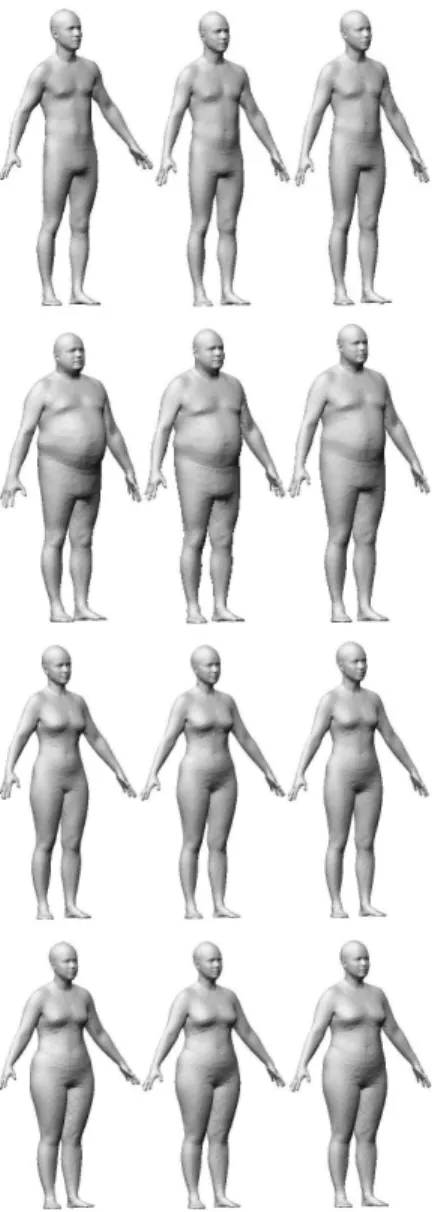
Figure 3. Shape prediction results. On each row from left to right: the original shape, predicted shape using linear regression and predicted shape using PCT.

vector Eregression is calculated for comparison to EP CT.

The comparison made in Figure 2 shows a close prediction accuracy between the linear regression approach using 44 measurements and the weighted PCT using 19 demographic attributes.

Besides the comparison on prediction errors, we also compare visually the body shapes reconstructed through Equation 2. Figure 3 shows examples of male and female prediction using the linear regression and weighted PCT approaches. It is no wonder that linear regression creates shapes being close to the original because it uses 44 body measurements for constraints. The reconstructions using the weighted PCT also show a close shape as the original.

VI. PRUNEDPCTFOR BODY SHAPE ANALYSIS For shape analysis, we concentrate on the first ten com-ponents, among which we also limit our analysis to prin-cipal components 1, 2, 4, 5 and 8. The reason is that the other components within the first ten all relate to posture variations. Figure 4 shows the shape variations along the selected principal components, by blending the global mean shape and shapes at±3pλj(j = 1, 2, 4, 5, 8) [10]. P C1 is

showing shape variations between a short female body and a tall male body. P C2 shows weight gains mainly around the waist line with both arms opening up. P C4 displays longer arms and legs, and weight gains around the waist line. P C5 shows weight gains on the upper body, including torso and arms.

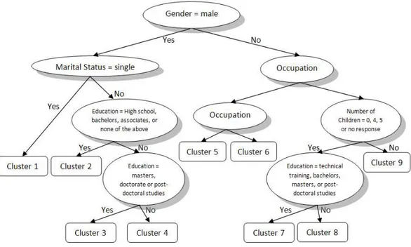
From the 19 demographic attributes listed in Table II, we select 6 of them for shape analysis (the third column). These attributes offers interesting analysis because they are related to shape but the relationship is not obvious. In contrast, the attributes in the first column are not related to shape and the attributes in the second column are directly related to shape. With the six selected demographic attributes, we rebuild the PCT and set the minimal number of cases in a leaf node to150. The pruned new PCT is displayed in Figure 5. From this tree we find that family income is not as related as the other five attributes because it is not used in any of the partition nodes.

The first interesting thing we find from the pruned PCT is that for males, body shape is mostly related to marital status and education being the second. For females, the most important factor is occupation, then number of children, leaving education the least related factor. It is also found that body shape in males is less affected by occupation than that in females.

We only put in Figure 5 those partition conditions having a short list of possible values, but list in full the following nine rules created by the pruned predictive clustering tree. The number at the end of each rule is the number of training cases in that cluster.

Rule 1 IF Gender = Male AND Marital-Status = ’ Single’ THEN [CLUSTER 1]: 355

Rule 2 IF Gender = Male AND Marital-Status in {’ Married’,’ Di-vorced’,’ Widowed’,’ Engaged’,’ No Response’} AND Educa-tion in{’ High School’,’ Bachelors’,’ Associates’,’ None of the above’} THEN [CLUSTER 2]: 292

Rule 3 IF Gender = Male AND Marital-Status in {’ Married’,’ Di-vorced’,’ Widowed’,’ Engaged’,’ No Response’} AND Educa-tion in{’ Masters’,’ Doctorate’,’ Post-Doctoral Studies’} THEN [CLUSTER 3]: 230

Rule 4 IF Gender = Male AND Marital-Status in {’ Married’,’ Di-vorced’,’ Widowed’,’ Engaged’,’ No Response’} AND Educa-tion in{’ Technical Training’,’ No Response’,’ Some College’} THEN [CLUSTER 4]: 158

Rule 5 IF Gender = Female AND Occupation in {’ Technician’,’ Administative Support’,’ Machine Operator’,’ Retired’,’ Unem-ployed’} THEN [CLUSTER 5]: 293

Rule 6 IF Gender = Female AND Occupation in{’ No Response’,’ Ser-vice Occupation’,’ Computer Programmer/Software Engineer’,’ Homemaker’} THEN [CLUSTER 6]: 150

PC1 PC2 PC4 PC5 PC8 Figure 4. Shape variations along selected principal components

Rule 7 IF Gender = Female AND Occupation in {’ Manage-ment’,’ Degreed Engineer’,’ Administrator’,’ Other Specialty Occupation’,’ Supervisor’,’ Attorney or Judge’,’ Transporta-tion OccupaTransporta-tion’,’ Student’,’ Scientist’,’ Sales/Marketing’,’ Classroom Teacher’,’ Mechanic’,’ Health Diagnosing Occupa-tion’,’ Armed Services’,’ ConstrucOccupa-tion’,’ Material Handler’,’ Other Legal/Judicial Occupation’,’ Training/Continuing Edu-cation’,’ Health Non-Diagnosing Occupation’,’ Farm Occu-pation’,’ Forestry or Fishing Occupation’} AND Number-of-Children in{0.0,4.0,’ No Response’,5.0} AND Education in {’ Technical Training’,’ Bachelors’,’ Masters’,’ Post-Doctoral Studies’} THEN [CLUSTER 7]: 306

Rule 8 IF Gender = Female AND Occupation in {’ Manage-ment’,’ Degreed Engineer’,’ Administrator’,’ Other Specialty Occupation’,’ Supervisor’,’ Attorney or Judge’,’ Transporta-tion OccupaTransporta-tion’,’ Student’,’ Scientist’,’ Sales/Marketing’,’ Classroom Teacher’,’ Mechanic’,’ Health Diagnosing Occupa-tion’,’ Armed Services’,’ ConstrucOccupa-tion’,’ Material Handler’,’ Other Legal/Judicial Occupation’,’ Training/Continuing Edu-cation’,’ Health Non-Diagnosing Occupation’,’ Farm Occu-pation’,’ Forestry or Fishing Occupation’} AND Number-of-Children in{0.0,4.0,’ No Response’,5.0} AND Education in {’ High School’,’ Doctorate’,’ Associates’,’ No Response’,’ None of the above’,’ Some College’} THEN [CLUSTER 8]: 151 Rule 9 IF Gender = Female AND Occupation in {’

Manage-ment’,’ Degreed Engineer’,’ Administrator’,’ Other Specialty Occupation’,’ Supervisor’,’ Attorney or Judge’,’ Transporta-tion OccupaTransporta-tion’,’ Student’,’ Scientist’,’ Sales/Marketing’,’ Classroom Teacher’,’ Mechanic’,’ Health Diagnosing Occupa-tion’,’ Armed Services’,’ ConstrucOccupa-tion’,’ Material Handler’,’ Other Legal/Judicial Occupation’,’ Training/Continuing Edu-cation’,’ Health Non-Diagnosing Occupation’,’ Farm Occu-pation’,’ Forestry or Fishing Occupation’} AND Number-of-Children in{3.0,1.0,2.0,6.0,’ 7 or more’} THEN [CLUSTER 9]: 233

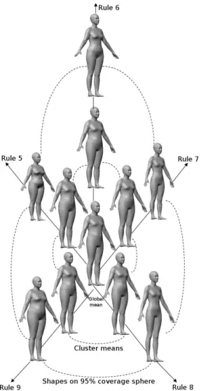
To have a better understanding of the actual body shape in each cluster, we reconstruct the (i) global mean shape, (ii) the shapes at the centroids of clusters, and (iii) the shapes being farthest from the global mean and inside the 95% covering sphere of each cluster. Figure 6 and 7

Figure 6. Male body shapes on cluster centers and 95% coverage spheres.

shows for males (Rules 1 to 4) and females (Rules 5 to 9) the reconstructed shapes described here. In each figure, the center body shape is the global mean and it is the same for males and females. The global mean shape is first

Figure 5. Pruned predictive clustering tree for shape analysis.

surrounded by shapes at the centroids of clusters, then by shapes meeting the criterion (iii) above.

Figure 6 shows that centroids and extreme shapes of Rule 2, 3 and 4 gained more body weight than those in Rule 1, which belongs to a cluster of single males. For those other than being single, subjects having education in “Masters, Doctorate, Post-doctorate” (Rule 3) have a lower body weight and height than those who do not have the education (Rules 2 and 4).

Figure 7 shows that a difference in occupation as de-scribed in Rules 5 and 6 creates two clusters of females in a different height. According to the pruned tree, clusters 7 and 8 as a whole have less number of children than cluster 9. The reconstructed shapes show that females in clusters 7 and 8 have a lower body weight than cluster 9. Between cluster 7 and 8, the attribute difference is on education (according to the tree) and the shape difference is mainly on body height (according to Figure 7). The female subjects having received a higher education (Rule 7) are lower in height than those who did not (Rule 8).

VII. DISCUSSION

In the weighted PCT, the first partition node is always gender. This is important in that the predicted body shape will have the right gender. If not using the weight, gender may not be the first partition node.

The predictive clustering tree also works in cases when both measurements and demographic attributes are avail-able. Adding body measurements to the training set grows the predictive clustering tree. When a set of attributes or

measurements are missing, the clustering tree can make a prediction by combining its leaf clusters.

In shape analysis according to the demographic attributes, the induction rules for males are easier for reading than those for females. Occupation as the main factor for clustering females has more possible attribute values than the rest of the demographic attributes. This prevents us from comparing between a combined cluster (clusters 5 and 6) and another combined cluster (clusters 7, 8 and 9).

VIII. CONCLUSION

In this work, we propose a predictive clustering tree, which has proved to be a robust and flexible tool for body shape prediction. It is also a fine analyzer for relations from demographics to body shape.

Building a weighted predictive clustering tree yields sim-ilar prediction accuracy as the linear regression approach. Also note that the clustering tree uses only 19 demographic attributes and the linear regression uses 44 body measure-ments. What is common in this comparison is that both approaches use 50 principal components.

Analysis on relation between body shape and demo-graphic attributes creates some interesting findings. In anal-ysis to body shape, the most related demographic attributes through a pruned PCT are marital status and occupation for males and females respectively.

For males other than being single, higher education leads to human bodies with a lower weight. For females, occupa-tion does make the biggest difference; however, those with more children are likely to have a heavier weight.

Figure 7. Female body shapes on cluster centers and 95% coverage spheres.

Our future work may include conducting leave-one-out experiment on the demographic attributes and testing the shape prediction performance.

REFERENCES

[1] B. Allen, B. Curless, and Z. Popovi´c. The space of human body shapes: reconstruction and parameterization from range scans. ACM Transactions on Graphics, 22(3):587–594, 2003. [2] B. Allen, B. Curless, and Z. Popovi´c. Exploring the space of human body shapes: data-driven synthesis under anthropo-metric control. In Proc. Digital Human Modeling for Design and Engineering Conference, 2004.

[3] B. Amberg, R. Knothe, and T. Vetter. Expression invariant face recognition with a morphable model. In Proc. FG’08, pages 1–6, 2008.

[4] D. Anguelov, P. Srinivasan, D. Koller, S. Thrun, J. Rodgers, and J. Davis. Scape: Shape completion and animation of

people. ACM Transactions on Graphics, 24(3):408–416, 2005.

[5] Z. Azouz, M. Rioux, C. Shu, and R. Lepage. Characterizing human shape variation using 3d anthropometric data. The Visual Computer, 22(5):302–314, 2006.

[6] A. Balan and M. Black. The naked truth: estimating body shape under clothing. In Proc. ECCV’08, pages 15–29, 2008. [7] V. Blanz and T. Vetter. A morphable model for the synthesis of 3d faces. In Proc. SIGGRAPH ’99, pages 187–194, 1999. [8] H. Blockeel, L. De Raedt, and J. Ramon. Top-down induction of clustering trees. 15th Int’l Conf. on Machine Learning, pages 55–63, 1998.

[9] Y. Chen and R. Cipolla. Learning shape priors for single view reconstruction. In Proc. 3DIM’09, pages 1425–1432, 2009. [10] T.F. Cootes, G.J. Edwards, and C.J. Taylor. Active appearance

models. IEEE PAMI, 23(6):681–685, 2001.

[11] D. DeCarlo, D. Metaxas, and M. Stone. An anthropo-metric face model using variational techniques. In Proc. SIGGRAPH’98, pages 67–74, 1998.

[12] S. Dzeroski, V. Gjorgjioski, I. Slavkov, and J. Struyf. Analysis of time series data with predictive clustering trees. Knowledge Discovery in Inductive Databases, pages 63–80, 2007. [13] P. Langley. Elements of Machine Learning. Morgan

Kauf-mann, 1996.

[14] K. Robinette, H. Daanen, and E. Paquet. The caesar project: A 3-d surface anthropometry survey. In Proc. 3DIM’99, pages 380–386, 1999.

[15] H. Seo and N. Magnenat-Thalmann. An automatic modeling of human bodies from sizing parameters. In Proc. SI3D’03, pages 19–26, 2003.

[16] H. Seo, Y. Yeo, and K. Wohn. 3d body reconstruction from photos based on range scan. In Proc. Edutainment’06, pages 849–860, 2006.

[17] J. Struyf, B. Zenko, H. Blockeel, C. Vens, and S. Dzeroski. Clus: User’s Manual. http://dtai.cs.kuleuven.be/clus/, 2010. [18] P. Xi, W.-S. Lee, and C. Shu. Analysis of segmented human

body scans. In Proc. GI’07, pages 19–26, 2007.

[19] P. Xi, W.-S. Lee, and C. Shu. A data-driven approach to human-body cloning using a segmented body database. In Proc. PG’07, pages 139–147, 2007.

[20] P. Xi and C. Shu. Consistent parameterization and statis-tical analysis of human head scans. The Visual Computer, 25(9):863–871, 2009.