Automated reasoning about classical mechanics

Automated Reasoning About

by

Leon Chih Wen Wong

Submitted to the Department of Electrical Engineering and

Computer Science

in partial fulfillment of the requirements for the degree of

Master of Science in Computer Science

at the

MASSACHUSETTS INSTITUTE OF TECHNOLOGY

May 1994

oc

Massachusetts Institute of Technology 1994. All rights reserved.

/e I

Deparmen.

.

.ri.g

_and'.

Department of Electrical Enginetg

and

iy1 /7

Computer Science

May 5, 1994

Certified by.. ..

Howard E. Shrobe

Principal Research Scientist

Thesis Supervisor

/".

Accepted by ... i

;

v...

...

Frederic R. Morgenthaler

Chairman, Departmental Committee on Graduate Students

Lng.

MASSACHiJ yi IN l,'rjJTN"T

I

Author

Automated Reasoning About Classical Mechanics

by

Leon Chih Wen Wong

Submitted to the Department of Electrical Engineering and Computer Science on May 5, 1994, in partial fulfillment of the

requirements for the degree of Master of Science in Computer Science

Abstract

In recent years', researchers in artificial intelligence have become interested in replicat-ing human physical reasonreplicat-ing talents in computers. One of the most important skills in this area is the ability to predict how physical systems behave. This thesis discusses an implemented program that can generate algebraic descriptions of how systems of rigid bodies evolve over time. Discussion about the design of this program identifies a powerful physical reasoning paradigm and knowledge representation approach based on mathematical model construction and algebraic reasoning. This paradigm offers a number of advantages over methods that have become popular in the field, and seems a promising approach for reasoning about a wide variety of classical mechanics problems.

Thesis Supervisor: Howard E. Shrobe Title: Principal Research Scientist

Acknowledgments

1 would like to thank Thomas Stahovich and Randall Davis for their valuable help with many aspects of my research. Special thanks go to Howard Shrobe, my supervisor, for his insight and guidance over the course of this project.

This research was conducted at the Massachusetts Institute of Technology Arti-ficial Intelligence Laboratory. It was supported by the Advanced Research Projects Agency of the Department of Defence under Office of Naval Research contract number N00014-91-J-4038.

Contents

1 Introduction

1.1 Background.

1.2 Project Goals ... 1.3 Thesis Organization... 2 AMES System Description

2.1 Introduction. 2.2 Task Description.

2.3 Design Overview ...

2.4 Introductory Example ...

2.5 Detailed System Description ... 2.5.1 Overview ...

2.5.2 Contact Analysis ... 2.5.3 Kinematics Analysis ... 2.5.4 Dynamics Analysis ... 2.5.5 Newtonian Mechanics ... 2.5.6 Reference Frame Semantics 2.5.7 Coordinate Systems Semantics 2.5.8 Subsequent State Generation 2.5.9 Summary ...

2.6 Examples ...

2.6.1 Particle on a Wedge ... 2.6.2 Two Blocks in a Corner . . .

15 15 17 18 19 ... . 19...

...

19

... . .21

... ....

3329

... . 37

... ..38

... ....

4239

... . .46

...

...

...

2.6.3 Particle on a Curved Surface ... 3 Extensions to AMES

3.1 Overview .

3.2 Representation and Reasoning .

3.2.1 Introduction...

3.2.2 Knowledge Representation 3.2.3 Inference Methods . 3.2.4 Reasoning Extensions . 3.3 Mechanics Domain Knowledge . .

3.3.1 Principles in Organization 3.3.2 Extending AMES' Domain 4 Directions for Future Research

4.1 Overview ...

4.2 Reasoning Efficiency ... 4.2.1 Problem Overview . .

4.2.2 Research Agenda ... 4.3 More General Reasoning ... 4.3.1 Problem Overview .... 4.3.2 Research Agenda ... 4.4 Modeling and Re-Representation

4.4.1 Problem Overview . .

4.4.2 Research Agenda ... 4.5 Other Areas for Research ...

K. . . . . . Knowledge 5 Related Research 5.1 Overview . ... 5.2 de Kleer: NEWTON .... 5.3 Kuipers: QSIM ... 5.4 Forbus: CLOCK and FROB

55 55 55 55 56 64 67 72 72 75 85

.... . 85

.... . 85

...

85

... .. 86

... ..

87

...

87

... .. 88

... .. 88

... .. 88

... .. 89

... .. 89

5.5 Novak: Physics Problem Solving Project ... 96

5.6 Addanki, Falkenhainer, Nayak: Modeling ... 97 5.7 Sacks and Joskowicz: Computational Kinematics ... 98

List of Figures

Components of State Analysis ... Particle on an Inclined Plane ... Summary of Contact Generation ... Coordinate System Conversion ... Example of State Change Ambiguity Contact Interaction Model Component Terrestrial Gravitation Model Component Newton's Second Law Model Component Newton's Third Law Model Component. Particle on a Wedge ...

Wedge Free Body Diagram ... Particle Free Body Diagram ... Corner Problem ...

Particle on a Sphere ... 3-1 Spring Example ...

3-2 Rope Contact Dynamics ....

2-1 2-2 2-3 2-4 2-5 2-6 2-7 2-8 2-9 2-10 2-11 2-12 2-13 2-14

... . .23

... ...44

... ..45

... ..45

... ..46

... .. ... ..48

List of Tables

Chapter 1

Introduction

1.1 Background

Much of human behavior involves interactions with the physical world. From space flight to microelectronics, some of humanity's finest intellectual achievements have been directed toward understanding our physical environment and manipulating it for an amazingly diverse number of different purposes.

It is hardly surprising, therefore, that researchers in artificial intelligence should seek to replicate human physical reasoning skills in computers. With such abilities, computers might provide intelligent assistance to engineers, interact more effectively

with their physical environment, and better understand the physical metaphors that

underlie much of human cognition.

Physical reasoning can be separated into two broad categories: design and analy-sis. Analysis represents the ability to understand how physical systems behave, while design represents the ability to create physical systems that act in some desired fash-ion. Both exist as areas of active interest in the artificial intelligence community; however, much of the work to date, including this thesis, has focused on the analysis portion of the task. The reason is quite simply that in human experience, understand-ing physical systems has been essential to effectively manipulatunderstand-ing them to meet our

goals.

role of performing numerical simulation from mathematical models. While this has been immensely useful, computers have been much less successful at higher level tasks such as creating the mathematical models to simulate, and interpreting the results. Furthermore, there are many cases where numerical reasoning is inappropriate or impossible: for example, situations where information is incomplete. Such cases are

common in the early stages of design, and when parameters of real world systems are difficult to measure. A related drawback to numerical reasoning is that the results are too specific to generalize in any way.

In the quest to extend computers' physical reasoning skills, researchers have used the abilities of human engineers as a source of inspiration. Engineers are physical reasoning specialists: they combine common sense intuitions, formal training, and expertise from practical experience to attack the complexity of physical systems. Examples of human skills that artificial intelligence researchers have sought to emulate include:

* Reasoning at multiple levels of abstraction * Accommodating incomplete information

* Constructing models of physical systems that simplify reasoning by describing properties relevant to the task at hand, but at the same time hiding irrelevant complexity.

* Solving problems efficiently by adapting solutions from past experience.

In addition to examining the reasoning paradigms used by engineers, researchers have also sought to duplicate the physical domain knowledge that people bring to bear on physical reasoning tasks. In particular, many have studied physical intuitions: those skills that allow even people with no formal training to interact effectively with their physical environment. In addition to their power in supporting everyday activities, this kind of common sense reasoning often guides engineers, the physical reasoning elite, in their application of more formal methods of analysis.

1.2 Project Goals

'The goal of this thesis was to investigate methods for solving analysis problems in classical mechanics. There were several reasons behind this choice of problem domain. One of the main motivations was that classical mechanics explains a large portion of the physical phenomena that people encounter in their regular activities. For this reason, methods for analyzing problems in this domain might offer a wide range of potential applications.

For the same reason, people have highly developed intuitions about mechanics that .help them understand other physical sciences. This suggests that studying classical mechanics might offer insights into reasoning effectively about other domains. Yet another reason for examining this domain is that as a result of centuries of study, peo-ple understand classical mechanics exceptionally well. This allows research to focus on issues solely related to transferring an understanding of the domain to computers. Lastly, despite the fact that mechanics scenarios are relatively simple to describe, they are capable of producing an interestingly complex array of behavior that challenges

the state of the art.

Given the focus of this thesis on classical mechanics, my research has specifically addressed three elements:

* Formalizing the knowledge required to understand classical mechanics. * Representing this knowledge in an effective manner

* Developing inference techniques that can effectively apply represented domain knowledge to solving analysis problems

One of the primary difficulties in investigating these aspects remains the fact that, despite the wealth of formal methods for analyzing the domain, much of hu-man perforhu-mance depends on poorly understood intuitions. Some of the challenges in automating classical mechanics reasoning therefore include substituting appropri-ate computer knowledge and inference methods for human physical intuitions, and interfacing these with the field's traditional formal methods.

Complicating this effort is the fact that computers display a very different set of strengths and weaknesses from people. This opens the door to certain powerful ap-proaches, such as computationally intensive algebraic techniques, but also complicates efforts to duplicate many human problem solving faculties.

1.3 Thesis Organization

This document describes research efforts toward the goals presented in the previous section. The next chapter describes AMES (Algebraic MEchanics Simulator), an implemented program that can reason about a limited range of classical mechanics problems. The chapter that follows distills the key features from AMES' design and illustrates how these principles might be generalized to expand the system's reasoning capabilities. This discussion also highlights many of the strengths and weaknesses of AMES' approach to physical analysis.

Chapter 4 builds on this evaluation of AMES' abilities by outlining some areas for future research. Following this, the last two chapters of the thesis look at how my research relates to other work in the field, and provide some concluding remarks.

Chapter 2

AMES System Description

2.1 Introduction

This chapter presents a description of AMES (Algebraic MEchanics Simulator). AMES is an implemented software system that can predict the behavior of a small range of scenarios from classical mechanics. It was designed to explore issues in effectively capturing and applying knowledge about this domain.

The next section describes the specific tasks and issues that AMES was designed to address. Section 2.3 provides an overview of the major features of AMES' design. Section 2.4 demonstrates how these elements interact in analyzing an introductory example. Following this is a detailed description of the system's architecture. Finally, the chapter ends with some examples that illustrate the range of AMES' capabilities.

2.2 Task Description

The previous chapter explained that the goal of this research project was to study

knowledge, representations, and inference methods for reasoning about classical me-chanics. The AMES program addresses these objectives by focusing on a single task: generating descriptions of how classical mechanics systems evolve from specifications of their initial conditions. This simulation problem was ideal for two reasons. First, understanding how systems evolve over time is a fundamental component of most

reasoning tasks in classical mechanics. Second, although simulation requires thor-ough knowledge of the domain, the problem model itself is relatively simple and constrained.

Note that two features differentiate AMES from numerical simulators, despite the fact that they share behavior prediction as their objective. First, AMES' input

con-sists of high level information appropriate for discussing classical mechanics systems: the objects in the scenario, and the values of their various static and dynamic at-tributes like shape, velocity, and field strength. AMES must therefore understand the relationship between system characteristics and the behaviors they generate. Numer-ical simulators, on the other hand require mathematNumer-ical models and initial variable values as input. The user must do all the reasoning about behavior in the domain to create these models; therefore, the simulators themselves have no physical knowledge. The second major difference from numerical simulators is that AMES was de-signed to accommodate information at a level of detail comparable to that found in introductory mechanics textbook problems. In particular, AMES handles scenarios described using algebraic, as opposed to numerical quantities. This is interesting from a research perspective for the same reason that educators teach the material in this fashion. Algebraic quantification accommodates a degree of incomplete information, allows one to generalize over ranges of parameter values, and produces not only so-lutions, but also the factors on which they depend. The ability to use algebraic, as opposed to numerical reasoning, therefore, appears important to emulating some of the human skills that have inspired researchers in physical reasoning.

Due to the limited resources for this project, however, AMES reasons about only a narrow subset of the classical mechanics domain: frictionless two-dimensional rigid bodies with no rotational degrees of freedom. Furthermore, although the system detects collisions, it does not predict their consequences. Lastly, AMES cannot ac-commodate ambiguity in the possible behaviors a physical system might exhibit. This kind of situation can occur whenever there is insufficiently detailed information about the values of the parameters of physical systems.

sufficiently complex to raise issues of very general interest. Subsequent chapters will outline how the principles learned from this simple system's design can be extended to overcome many of the prototype's defects and limitations.

The following two sections outline the key elements of AMES' architecture, and present a brief illustration of how they work together to solve a simple mechanics problem. Section 2.5 elaborates on this with a much more detailed description of the system's reasoning, and more complex examples.

2.3 Design Overview

This section describes the high level organization of the Algebraic MEchanics Simu-Ilator (AMES). As mentioned in the previous section, AMES was designed to predict the behavior o:f mechanics systems from physical descriptions of their initial configu-rations.

AMES shares the same general reasoning paradigm as numerical simulators. It predicts the behavior of physical systems incrementally: information about each suc-cessive time interval in a scenario's evolution comes from the analysis of its prede-cessor. A unique feature about AMES, however, is that the granularity of simulation time intervals is much more coarse that those in numerical simulation. While numer-ical simulators reason about the changes that occur over very small fixed length time intervals, AMES reasons about changes that occur over longer variable durations of time called qualitative states.

In AMES, a qualitative state is a period of time over which one can describe the evolution of a physical system using a single mathematical model. This notion is

therefore sensitive to the power of the mathematical infrastructure supporting the

simulator, as well as the fundamental complexity of each physical system's behavior. The reason such states are termed "qualitative" in nature is that changes in what people recognize as the high level behaviors of a physical system typically translate into changes in the mathematics required to model them. For example, one might in-formally judge static and sliding friction to be qualitatively distinct behaviors. AMES'

knowledge-base would represent a similar distinction, though the criterion would be more objective: a transition between the two conditions implies a change in the math-ematical description of frictional force. For the static case, friction balances all other forces in the direction parallel to the contact generating the force, in the contact frame of reference. Sliding friction, however is proportional to contact normal force, and is directed opposite the direction of relative motion.

The definition of qualitative states in terms of mathematical models is more than an attempt at formalizing informal notions of qualitative distinctiveness, however. The main reason for this manner of partitioning simulation histories is that AMES constructs mathematical models to reason about the behavior of physical systems. It is not always the case, however, that a single model can describe the entire evolution of a system. Therefore, AMES must partition its envisioning into intervals over which individual models hold.

Given this kind of reasoning scheme, the central element in AMES' simulation procedure is naturally the individual qualitative state analysis: the process by which AMES models a system's behavior during a state, reasons about how that state ends, and generates information to support similar analysis of its successor. Each successive application of this procedure pushes the simulation another qualitative state further into the future. Note that although AMES operates at a higher level of abstraction, this organization of reasoning is very similar to that found in Qualitative Simulation

[211: a technique for qualitatively solving systems of differential equations.

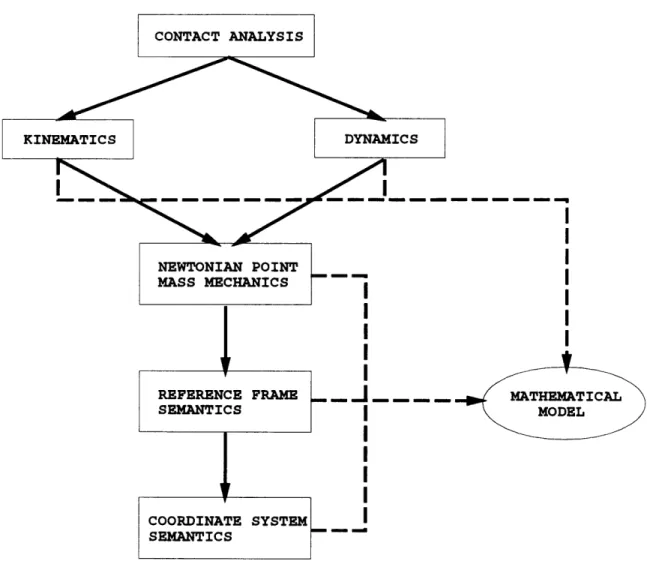
As was just mentioned, the state analysis process begins with constructing a mathematical model that describes how attributes of a physical system will evolve over the course of that state. Model construction proceeds in several stages. Figure 2.3 illustrates the organization of the process. The schematic reflects both the structure of domain knowledge within AMES, and the flow of information during model assembly. Each module in the state analysis examines a different aspect of a physical system, and each can generate information of three different types. Modules may conclude qualitative information about the current state: for example, that contact between two objects exist. Modules can also generate quantitative information: sets of

con-_I

__ X _

_ -

--

I

I

Module Description

Contact Analysis Determines the contacts in the scenario Kinematics Determines restrictions on bodies motions Dynamics Describes the forces in the scenario

Point Mass Mechanics Applies Newton's laws, and relates motion attributes to each other

Reference Frame Semantics Relates quantities measured in different reference frames

Coordinate System Semantics Relates quantities measured in different co-ordinate systems

Table 2.1: Module Descriptions

straints to incorporate into the mathematical model of the state. Finally, modules may generate state termination conditions: specifications of the events that would force changes to the model. Table 2.3 summarizes the role of each analysis module in AMES.

Once AMES generates a mathematical model of a qualitative state, the next step is to determine when and how the state ends. As previously mentioned, during the model construction phase, analysis modules generate state termination conditions that indicate when each part of the model contributed by those modules becomes invalid.

AMES therefore detects the end of the state by simply solving for when, if ever, the first state termination condition occurs. Then, AMES uses the current model to solve for the initial configuration of the subsequent state. The analysis of the next qualitative state uses these initial conditions along with information about the

transition that created the state change as input.

The next section outlines the how AMES follows the above pattern of reasoning to analyze a simple physical scenario. The section after that explores the details of AMES' operation.

Ž

0,~"

t

the top of the plane, it can use the same model for reasoning about the scenario as long as the particle contacts that particular side of the incline. The range of validity of the model also determines the scope of the qualitative state, by definition.

From the contact configuration, AMES can deduce information about the state's kinematics and dynamics. Since the state lasts as long as the contact is present, it is possible to add equations to the model that establish that the particle's velocity will be tangential to the top of the incline. The usefulness of this information resides in the way it constrains the value of the normal forces between the bodies.

In analyzing the situation's dynamics, the existence of the contact establishes the existence of contact forces. From AMES' knowledge about these forces, it asserts that their direction is perpendicular to the contacting surfaces. The magnitude of the contact forces comes indirectly from the kinematic constraint: they take on whatever value is necessary to keep the particle moving tangentially to the surface of the incline. This is AMES' method for defining the behavior of compensating forces.

Note, however, that this model is not always accurate: contact normal forces only repel. Therefore, if there were a force that pulled the two bodies apart, the normal force could not resist. The particle would acquire velocity away from the incline, and therefore not move tangentially to its surface, producing a contradiction. This is where reasoning about model limitations enters. AMES handles the potential problem by having a termination condition that states that the model must change if it predicts attractive contact normal forces.

The other element to the system's dynamics, aside from the contact forces, are the gravitational forces. AMES has knowledge that gravity acts on each rigid body in the scenario with a value equal to the product of the field's strength and each body's mass.

At this time, AMES has all behaviors in the scenario reduced to information about forces, and constraints on bodies' motions. It can therefore proceed to apply Newton's laws by relating action-reaction force pairs, and performing free body analysis of each body. This stage of analysis also adds to the model information about the derivative relationships between positions, velocities and accelerations.

The last step in the model construction process is to add reference frame and coordinate system conversions. These are necessary because AMES' model typically has multiple variables representing different ways of measuring the same attributes. This apparent redundancy is useful because it is very convenient to discuss contacts, for example, in terms of relative motions between contacting bodies in parametric coordinates, while it may be more natural to discuss other behaviors, such as Newton's second law, in terms of inertial reference frames and cartesian coordinates.

When the modeling process is complete, AMES turns to reasoning about state change. The mathematical model it generated is only valid as long as the same contact configuration persists. AMES therefore has two types of conditions on the duration of the initial qualitative state: conditions that establish that no new contacts occur, and conditions that establish how long the existing contact persists. In this case, it is clear that no new contacts occur, since the only other possible contacts are between the particle and the other sides of the incline: these cannot happen since the sides occupy mutually exclusive portions of space. The old contact, on the other hand has 3 potential ways to end: the particle can move off the end at either the top or the bottom, or it might fly off in the middle.

The first two conditions are constraints on position, while the normal force magni-tude constraint that was mentioned earlier implements the last condition. In the case of this scenario, AMES has enough information to solve for the fact that the particle in fact slides off the bottom of the incline. The state change therefore involves an end to the contact, and the next state has an empty contact configuration.

The analysis of the next state therefore concludes that the particle is in free fall. Furthermore, the direction of the particle's motion is such that new contacts are impossible. Therefore, the free fall state never terminates and the simulation is complete.

2.5 Detailed System Description

2.5.1 Overview

This section describes AMES' simulation procedure in detail. Note, however, that the implemented system queries the user for all mathematical reasoning tasks. The reason for this was that automated algebraic reasoning is fairly well understood, and therefore efforts in this area were unlikely to further this project's research goals. To ensure that the system's performance is still convincing, however, AMES has its own representation of mathematical objects, and all quantitative reasoning occurs through a narrow interface: either solving for the value of a variable or determining the truth of an expression.

The description of AMES in this section consists of several subsections. Each subsection illustrates the operation of a different component of the analysis procedure. The first several describe the different model construction modules. They each discuss the following aspects of the modules' operation:

* The aspect of physical scenarios that the module examines.

* The inference techniques used to perform the analysis.

* The contributions to the mathematical model of the state.

* The conditions on the validity of the analysis.

After the descriptions of the individual model construction modules, this section discusses how AMES uses its mathematical models of qualitative states to provide information for the analysis of their successors. The section closes with a summary of AMES knowledge about mechanics.

2.5.2

Contact Analysis

Scope

As the name implies, the contact analysis module produces a description of the various contacts between rigid bodies in the current state. This information is critical since it allows the system to deduce the presence of normal forces and various motion constraints. In AMES' limited domain, changes in contact configuration completely determine changes of qualitative state, since the program assumes that all the other highest level behaviors, namely gravitation and externally constrained factors, remain constant over the course of simulations.

When a contact exists between two objects, the contact module computes the locus of relative positions that allow the bodies to remain in contact. The shape of the contact locus, in turn, allows other parts of the state analysis to find the direction of surface normal forces, and the range of motions that the impenetrability of rigid bodies allows.

A very natural way to represent contacting positions is to compute the shapes of objects in other objects' configuration spaces [23]. This method reduces the problem of finding contacts in AMES' domain to the geometric problem of determining whether a point lies on the edge of a two-dimensional shape. Another advantage of this scheme is that features such as normal force directions remain unchanged by the configuration space transformation.

Note, however, that the outlines of shapes typically found in mechanics problems are often discontinuous: for example the discontinuities at the corners of a rectangular block. This prevents straightforward mathematical characterization of the entire ]ocus of contact positions, and therefore complicates the mathematical modeling task. AMES' solution, therefore, partitions sets of contacting positions into piecewise simple segments, where "simple" is defined by the ability of the geometric analysis module to produce purely mathematical descriptions of each resulting shape. The rest of this thesis will refer to these subsets of contacting positions as simple contacts.

bodies in each qualitative state. Note that unlike many of the other analysis modules, the contact analysis makes no direct contribution to the mathematical model. Instead, it provides information to the kinematics and dynamics modules. They, in turn, interpret the consequences of the contacts in terms of restrictions on bodies' degrees of freedom, and normal forces between contacting objects.

Inference Methods

AMES employs a straightforward technique for finding simple contacts and computing their shape. Before the simulation begins, AMES generates descriptions of all possible simple contacts that can occur between the rigid bodies in the problem scenario. During the simulation, the contact analysis module describes contact configurations by maintaining sets of pointers to the simple contacts that are actually present during each state. AMES actually needs information on all possible contacts since accurate modeling depends on knowing not only the current contact configuration, but also what new contacts might appear.

To generate all the possible contacts, AMES considers every possible pairing of rigid bodies. For each pair, it selects one object to be the "observer". The other object becomes the "obstacle". Then, AMES computes the shape of the obstacle in the observer object's configuration space. This gives the shape of the locus of contacting relative positions for that pair of objects.

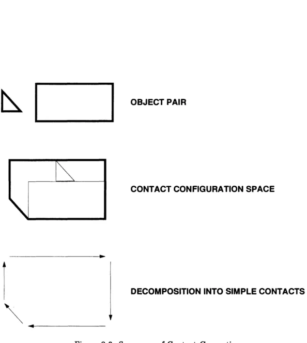
Once the obstacle configuration space shape has been computed, the outline of the shape is decomposed into simple segments: shapes for which the quantitative rea-soning engine can find mathematical descriptions. The current mathematics module supports two types of one-dimensional shape primitives: circular arcs and line seg-ments. Therefore, all configuration space obstacle shapes are decomposed into these. Note that the decomposition is always possible since all of the rigid object shapes are also composed entirely from these primitives. Figure 2.5.2 gives a graphical summary of the contact generation process.

A small subtlety of this process is that the simple contact shapes are stored as directed paths. The direction information allows AMES to record which side of the

OBJECT PAIR

CONTACT CONFIGURATION SPACE

DECOMPOSITION INTO SIMPLE CONTACTS

Figure 2-3: Summary of Contact Generation

path corresponds to the exterior of the obstacle object. This information is critical in determining the direction of normal forces between the contacting bodies.

An additional issue in the contact generation is choosing observer and obstacle roles for each pair of objects. This choice is actually unimportant in terms of pro-ducing a correct analysis, since the configuration space computation is commutative [23]. AMES does, however, use a heuristic to assign the role of "obstacle" to the ob-ject whose shape most resembles its configuration space shape: it makes the smaller object the "observer". This makes the analysis somewhat easier for human users to

follow.

During the simulation, AMES checks for the existence of various contacts by considering the configuration space position of each observer object in the reference frame of their corresponding obstacles. If the position happens to be on a simple contact, then the system deduces that that contact appears in the state. Between states, if there is no evidence that a contact has been broken, then AMES simply carries the contact into the next state: there is no need to repeat the analysis. Similar reasoning also applies to predicting the contacts that are not present.

Dependencies

For a particular set of contacts to remain an accurate description of a state, two facts must hold. First, no existing contact can break, and second, no new contact can appear. The validity of the contact analysis therefore depends on formal descriptions of these two conditions. New contacts are easy to detect during the simulation, due to the extensive processing during the initialization phase: the configuration space shapes that are generated before the simulation begins indicate the relative positions of objects that result in contacts. During the simulation, therefore, satisfying the existence criterion of a simple contact that does not appear in the current state invalidates the state's contact description and leads to a new state.

Detecting when existing contacts disappear, however, is slightly more difficult. Every simple contact is a finite length one-dimensional path consisting of positions that the observer can occupy and still preserve contact. There are therefore two

different ways to break an existing simple contact: the observer object can move beyond an endpoint of the contact path, or the observer can move off the path from

some internal point.

The first condition is simple to express mathematically, especially since AMES uses distances along simple contact paths to describe displacement. Expressing the

second condition turns out to be slightly more involved, however, because of the dif-ficulty of expressing rigid bodies' tendency to slide against each other. To describe that behavior, the kinematics module, as will be described below, has a model where contacting bodies must always stay connected. This means that the state's mathe-matical model does not permit velocities to have components normal to the simple contact shape.

The actual state termination condition is therefore expressed in terms of contact normal force direction. If a contact force must be attractive in order to preserve contact, then contact breaks. The section on dynamics analysis will explore the rationale behind this design in greater detail.

2.5.3 Kinematics Analysis

Scope

The concept of impenetrability is a key element of informal descriptions of rigid bodies. This characterization is incomplete in many ways, however. In particular, it says little about what mechanism prevents bodies from occupying the same space. AMES provides this missing information in the kinematics and the dynamics that it

associates with contacts.

The goal of the kinematics analysis is to refine higher level knowledge about

qualitative states into constraints on objects' motions. Within the scope of problems

that AMES addresses, this task translates into converting contact information and user specified motion restrictions into constraints on rigid body positions. AMES represents such degree of freedom restrictions with shapes that indicate the loci of positions that bodies can possibly occupy. These positions might be measured relative

to any reference frame. This gives the description format the flexibility required to clearly describe the relative position constraints that arise from contacts.

Inference Methods

The kinematics module collects degree of freedom restrictions from two sources: user-supplied information about external influences on the scenario (like the "glue" that attaches things like floors and walls to the fixed frame), and the state's contact configuration. In the first case, no special inference is required, since the information comes directly from the user.

Deducing degree of freedom restrictions from contact information is not much more complex. For each simple contact in the current state, it must be the case that as long as that contact persists, the bodies must have relative positions inside the configuration space shape that describes the contact. Therefore, the degree of freedom restriction has the same shape as the contact locus.

Model Contribution

The kinematics module adds a set of equations to the mathematical model of the state for every degree of freedom restriction present. In AMES's world of rotation-free two-dimensional geometry, there are only two types of degree of freedom restrictions:

zero-dimensional and one-dimensional.

In both cases, the motion constraints can be expressed as restrictions on objects' velocity. Zero-dimensional degree of freedom restrictions imply zero velocity, while one-dimensional degree of freedom restrictions imply that velocity must always be tangential to the path restriction: otherwise the object would move off the path. Note that the reason that AMES uses velocity constraints is that the equations tend to be simpler to express than the more fundamental position constraints. With the proper initial conditions, however, the two formulations are equivalent.

Dependencies

AMES assumes user-specified phenomena persist over the entire course of a simula-tion, therefore there are no state transition conditions to associate with these. For kinematic constraints from contacts, the conditions that guarantee contact are suffi-cient to ensure the correctness of the kinematic analysis.

2.5.4 Dynamics Analysis

Scope

The dynamics analysis determines the forces that act in the current state, and infers constraints on their values. AMES scenarios can contain three types of forces:

* Gravitational forces: the effects of gravitational fields on rigid bodies.

* Contact normal forces: the repulsive forces that prevent penetration and defor-mation of rigid bodies.

* External forces: forces from sources other than the participants in the scenario.

These are specified by the user directly, or come from user-specified kinematic

constraints.

Inference Methods

AMES builds dynamics descriptions in two phases. The first phase enumerates the forces that the current state contains. The second phase produces information on their values. This subsection discusses the first phase. The following subsection describes the second.

In AMES's limited universe, it is very simple to deduce the existence of forces. External forces come from two sources. The easiest to identify are those that the user specifies directly. For example, a scenario might have a block pushed by some force 'that arises from interactions outside the system: the user must therefore explicitly tell AMES about the force's existence. The second class of external forces that AMES

detects come from motion restrictions imposed by outside sources. These motion restrictions must have reaction forces that provide the necessary constraints.

The existence of gravitational forces are just as easy to infer: the dynamics module deduces a gravitational force for every unique pairing of a rigid body with a gravita-tional field. Lastly, AMES postulates an action-reaction pair of contact normal forces for every contact in the current state.

Model Contribution

AMES adds equations to the mathematical model that describe each force present in the current state. For user-specified forces, the system simply asserts that the force has its user-provided value. For forces that enforce user-specified motion constraints, no equations are necessary: Newton's second law constrains them to have whatever values necessary to enforce the motion constraints they support. For gravitational forces, AMES asserts that the force value is the value of the gravitational field, scaled by the mass of the object on which each force acts.

Only contact normal forces make a somewhat complex contribution to the math-ematical model. AMES asserts that each contact force has no component tangential to the contact locus that generates it. In other words, each contact force must have a direction that is normal to its corresponding contact: hence their description as

"normal" forces.

This definition intentionally leaves undefined the magnitudes of the contact forces. The reason is that normal forces are compensating forces: they adopt the minimum magnitude necessary to prevent rigid bodies from penetrating each other. Ensuring that the bodies move tangentially along the contact locus represents this "minimal" effort. Therefore, the kinematic constraints determine the normal force magnitudes.

Dependencies

AMES assumes that gravitational fields and external forces are permanent. Therefore, initial deductions need never be changed. Since their semantics are so simple, those deductions do not depend on any special conditions for validity.

Normal forces change with states' contact configurations; however, as long as a particular set of contacts persists, the above deductions surrounding normal forces remain valid. Note the formulation of normal forces appears to leave open the possi-bility of attractive normal forces, when textbook-style knowledge states that normal forces can only be repulsive. To understand why this is not a problem, recall that when normal forces become attractive, the contact module understands that this is a sign that the contact is breaking. The justification is that normal forces would only be attractive if the bodies had some tendency to move apart. Therefore, qualitative states always end before normal forces become attractive.

2.5.5 Newtonian Mechanics

Scope

The Newtonian mechanics module is responsible for relating quantities in the state by applying Newton's laws of motion wherever possible. Note that although there are three laws of motion, the first law is merely a special case of the second law. The first law states that objects have uniform velocity unless acted upon by external unbal-anced forces. The second law states the mass of a body multiplied by its acceleration, measured from an inertial reference frame, is equal to the sum of the incident forces on that body. When the sum of the incident forces is zero, the second law is identical to the first law. The Newtonian analysis module therefore only records instances of the second and third laws.

In addition to applying these constraints, this module also generates the differen-tial equations that represent the derivative relationships between acceleration, veloc-ity, and position.

Inference Methods

The Newtonian mechanics module generates all possible instances of Newton's sec-ond law by essentially performing a free body analysis of every rigid body. This involves retrieving all the incident forces on each body from the dynamics module.

Similarly, it constructs every possible instance of Newton's 3rd law by retrieving from the dynamics module every action-reaction force pair. Action-reaction pairs can be identified by their mirrored source-target relationship, and similarities in force type and point of interaction.

Model Contribution

The Newtonian analysis module generates very straightforward textbook-style equa-tions for each law instance. For Newton's second law, it asserts that the sum of the incident forces equals the mass of a body multiplied by its acceleration. For Newton's third law, it asserts that the values of action and reaction forces are vector negations of each other.

There is a subtlety worth noting about the process, however. AMES states each law in a canonical style: it describes all quantities with respect to the fixed inertial reference frame, using cartesian coordinates. This simplifies the instantiation process,

and relies on the conversion modules to relate the results of the law's constraints to

variables representing differently measured versions of the same physical attributes. As previously mentioned, this analysis module also contributes equations that describe the derivative relationships between position, velocity, and acceleration. Note that neither Newton's laws nor the relationships among motion attributes introduce new restrictions on the validity of the model of the qualitative state.

2.5.6

Reference Frame Semantics

Scope

This analysis module defines the semantics of reference frames by providing knowledge about how to convert quantities between reference frames. AMES allows reference frames to be attached to any rigid body in a scenario. The ability to measure quan-tities in different reference frames allows compact representations of many aspects of the behavior of mechanics systems. For example, contact properties are very easy to describe in terms of relative positions. Relative positions, in turn, can be expressed

cleanly in terms of one object's position in another's object's reference frame.

Inference Methods

During the simulation, the task of the reference frame conversion module is to add equations to states' mathematical models that relate variables that represent mea-surements of the same quantities in different reference frames. Although there are many ways to accomplish this task, AMES operates by relating all attributes in the mathematical model to their values measured in a common reference frame: the fixed frame.

Model Contribution

AMES measures only attributes that describe motion against reference frames. For each of position, velocity, and acceleration, the conversion equations have the same format. The attribute's value in the standard frame of reference is the sum of its value in the non-standard reference frame, plus the non-standard reference frame's value in that kind of attribute, measured against the fixed frame. If the reference frame's value in the attribute is not measured with respect to the fixed frame, it can be obtained by applying the same conversion process. Naturally the conversions depend on there being some sequence of intermediate reference frame relationships that eventually terminates with the fixed frame.

2.5.7

Coordinate Systems Semantics

Scope

The coordinate system analysis module contains knowledge about coordinate system semantics in its ability to mathematically relate measurements of quantities from different coordinate systems, but identical reference frames.

AMES supports two types of coordinate systems. For two-dimensional spaces, AMES uses traditional cartesian coordinates. It describes all cartesian coordinate systems by an offset and a rotation relative to a distinguished coordinate system

associated with each reference frame.

AMES also supports specialized parametric coordinate systems that I term path

coordinates. Path coordinates simplify problems that involve determining the

behav-ior of bodies that are constrained to move along one-dimensional trajectories. Under path coordinates, attributes of a system are measured with respect to unit vectors that are tangential and normal to the trajectory at the location of the constrained body. The position of the body, however, is measured in terms of distance along the

path.

This system of measurement simplifies calculations since it separates the influ-ences on a body into components that cause it to translate along its trajectory, and components that cause the curvature of the trajectory. This arrangement also simpli-fies the task of reasoning about the effects of compensating forces: those forces that

constrain the body under observation to its designated path.

Inference Methods

The coordinate system analysis module provides the mathematical relationships be-tween quantities measured in different coordinate systems in much the same way as the reference frame conversion module. It works by generating equations that relate all measurements to their analogs measured against their reference frames' standard cartesian coordinate systems. Combined with the reference frame conversions, the process allows all different measurements of identical quantities to be mathematically

related.

Again, similarly to reference frame conversions, AMES applies coordinate system conversions to every quantity in the mathematical model that has been expressed in

a non-standard format. The next subsection discusses the structure of the conversion

equations.

Model Contribution

Conversions of both cartesian and path coordinates occur in much the same way. The major difference between the two lies in the fact that the rotation and offset of

Y

B

X

A

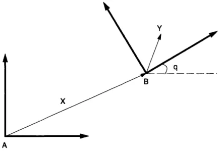
Figure 2-4: Coordinate System Conversion

the cartesian coordinate systems in AMES are constant, whereas in path coordinates they can be variable. The only other difference lies in each system's methods for measuring displacement.

For both types of coordinate systems, the conversion equations have much the same format. Displacement requires somewhat special treatment, however. The diagram below illustrates the general case.

For attributes other than displacement, AMES converts a quantity that has value Y in coordinate frame B by simply rotating Y by the rotation of coordinate system B, angle q. AMES must also add the offset vector X when converting displacements. For cartesian coordinates, AMES reads the offset and angle information from the description of the coordinate system. For path coordinates, this information comes from geometric operators that, given the parameterized position of an observing body along a trajectory, return the path angle and cartesian position.

2.5.8 Subsequent State Generation

When the mathematical model of a physical system in its current qualitative state is complete, AMES determines when the state terminates, and generates a description of the subsequent state. During the model construction process, the system accumulates a set of preconditions for the model's accuracy. Since states in AMES, by definition, persist only as long as the corresponding mathematical model remains valid, the current state terminates when the first model validity precondition fails.

To find this time, AMES simply attempts to solve for the time when each pre-condition fails. If there are no solutions, then the current state persists indefinitely, and the simulation terminates. Otherwise, AMES sorts the failing preconditions by time and considers the set of preconditions that fails first. A mathematical subtlety is that only those solutions that have times after the start of the state are valid, since the model itself is not valid before that time.

With the state termination time, AMES solves for the values of the positions and velocities of all the rigid bodies in the scenario. This information forms the basis for the initial conditions of the next state. Positions and velocities completely describe the configuration of the system, and have the property that they are continuous; therefore, their values do not change across the state boundary. This makes these attributes adequate for describing system configurations.

In addition to the values of these attributes, the state termination analysis provides key information about the qualitative properties of the subsequent state, based on the manner in which the previous state ends (i.e., the model precondition or preconditions that failed). This is necessary to the simulation process since the period of state transition is always at the boundary between different behaviors, and the information necessary to disambiguate them is not always contained in the positions and velocities alone.

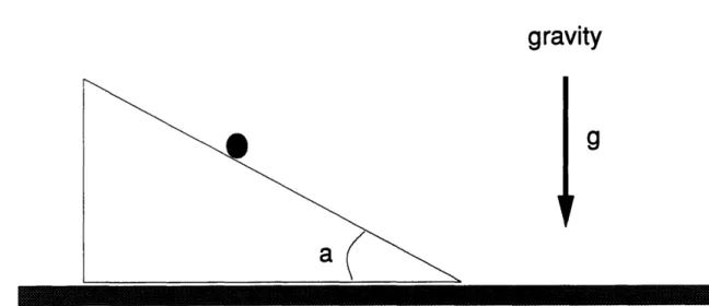
For example, consider the following scenario, where a particle is at rest touching the underside of a horizontal plane.

For this case, AMES creates an initial state during which the two bodies touch. As should be clear to the reader, this state terminates immediately; therefore, the initial

gravity

Figure 2-5: Example of State Change Ambiguity

conditions for the subsequent state are identical to the original initial conditions. Ad-ditional information is evidently necessary for the next state's analysis: in particular, the system needs to communicate information about how the previous state ended. In this case, we can exploit the knowledge that the initial state terminates because the normal force from the plane to the particle would have to be attractive in order to preserve contact. In other words, there is an applied force on the particle that draws the bodies apart. Therefore, in the simulation's second qualitative state, AMES can correctly assume a free fall situation.

This example suggests that position and velocity information are not sufficient to generate accurate descriptions of states at times of state transition. On the other hand, no more attributes of the subsequent states can be predicted by the previous state's analysis, since all other time varying attributes can change discontinuously across state boundaries. It is therefore important to employ facts about how state transitions arrive in order to describe new qualitative states.

As previously mentioned, it happens to be the case that for the range of prob-lems that AMES addresses, only assertions about contacts generate state termination conditions. Contacts in AMES are binary in nature: they are either present or not present. After a state terminates, therefore, it suffices to simply reverse the status of the contacts associated with the conditions that triggered the state change. We can assume that other contacts remain intact since their termination conditions were not met, and contact depends on position, which is a continuous attribute.

Model Component: Contact

Arguments

Rigid body: Bodyl. Rigid body: Body2.

Simple contact locus between Bodyl and Body2: Contact

Activation Conditions:

position(Bodyl,: wrt Body2) E Contact

Deactivation Conditions:

magnitude(NormalForce)

< 0

Qualitative Assertions:

There exists a force NormalForce from Bodyl to Body2.

Mathematical Assertions:

direction(NormalForce)

= angle(Contact,:

at position(Bodyl,: wrt Body2)) +

position(Bodyl,: wrt Body2)) E Contact

Figure 2-6: Contact Interaction Model Component

2.5.9 Summary

Figures 2.5.9 through 2.5.9 summarize AMES' high level knowledge about the me-chanics domain. They organize this information according to a representation scheme called model components that the next chapter will describe in detail. The model component representation arose from an analysis of AMES' reasoning paradigm and crystallization of its physical reasoning knowledge.

2.6 Examples

This section demonstrates the methods that AMES uses to analyze physical systems by discussing the program's ability to solve three sample problems. The examples illustrate the range of complexity that AMES can accommodate. The discussion surrounding each problem highlights the elements of the program's approach that provide its power.

Model Component: Terrestrial Gravitation

.Arguments:

Rigid body: Body. Gravitation field: Field.

.Activation Conditions: always

Deactivation Conditions: never Qualitative Assertions:

There exists a force GravForce from Field to Body. :Mathematical Assertions:

GravForce = :mass(Body) strength(Field)

Figure 2-7: Terrestrial Gravitation Model Component

:Model Component: Newton's 2nd Law

.Arguments: Rigid body: Body. Forces on Body: Forces.

Activation Conditions: always Deactivation Conditions: never Qualitative Assertions: none :Mathematical Assertions

EForces = Mass(Body) Acceleration(Body,: wrt FixedFrame)

Figure 2-8: Newton's Second Law Model Component

.Model Component: Newton's 3rd Law

Arguments:

Force of type Type from Bodyl to Body2: Forcel.

Force of type Type from Body2 to Bodyl: Force2.

Activation Conditions: always Deactivation Conditions: never Qualitative Assertions: none .Mathematical Assertions:

Forcel = -Force2

gravity

g

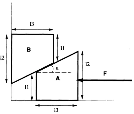
Figure 2-10: Particle on a Wedge

2.6.1

Particle on a Wedge

Consider the scenario depicted in figure 2.6.1. Assume that all bodies begin at rest, and that all contacts are frictionless. The ground's position is fixed, but the particle and wedge are free to move. Terrestrial gravity is present.

There are a number of complexities in this problem that make it interesting to examine:

* Solving for the normal force between the particle and the wedge is difficult, since both are non-inertial reference frames.

* The acceleration of the wedge depends on the magnitude of the normal force from the particle: a circular dependence.

* It is not entirely obvious whether it is possible for the wedge to slip out from underneath the particle and break contact.

As this section will discuss, however, application of AMES' methodical approach generates sufficient mathematical constraints to solve for the unknown forces and accelerations. This then permits the system to completely characterize all motions in the scenario. Together, these elements constitute a complete model of the physical system in its initial qualitative state.

Given the initial configuration of the scenario, AMES' first step is to identify all

the contacts. It finds the particle contacts the top of the wedge, and that the bottom

of the wedge contacts the ground. Furthermore, there are no initial velocities that would immediately break contact. This contact information allows the system to deduce a number of important facts.

In terms of the scenario's kinematics, the contact information allows AMES to

conclude that during the initial qualitative state:

* The velocity of the particle remains tangential to the top of the wedge.

* The velocity of the wedge remains tangential to the top of the ground.

Since the respective surfaces are straight, the derivative relationship between ve-locity and acceleration implies that the two bodies' accelerations are also constrained

to be tangential to their respective contacts.

In addition to these kinematic constraints, the contact information allows AMES to conclude the existence of normal force pairs between the wedge and the particle, and between the wedge and the ground. Also, AMES' domain knowledge constrains the directions of these forces to be perpendicular to the plane of their respective contacts. Note, however, that the normal force magnitudes cannot be directly determined at

this time.

Adding to the normal forces, AMES analysis of the scenario's dynamics concludes that gravitational forces influence all three rigid bodies. AMES can determine both the magnitude and the direction of each of these forces since it has information about

the bodies' masses and the gravitational field's strength.

At this point, all the high level interactions in the system have been expressed in terms of the kinematics and dynamics of each individual participant. Therefore, AMES is in a position to apply Newton's laws to the situation. Newton's third law equates the magnitudes of the members of each normal force pair. Newton's second law provides free body analysis of each object.

AMES performs free body analysis with respect to the fixed frame of reference to avoid the complications of reasoning about the fictitious forces that non-inertial

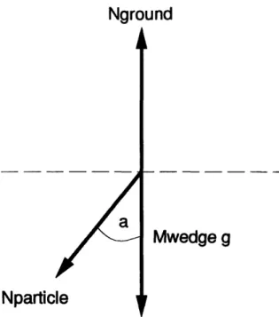
Nground

Npartic

Mwedge g

Figure 2-11: Wedge Free Body Diagram

reference frames require. Figure 2.6.1 shows the free body diagram for the wedge. Since the acceleration of the wedge is purely horizontal, the free body diagram pro-vides enough information to determine that the wedge's acceleration has strength

Npaticl in toward

the left.

Mwedge

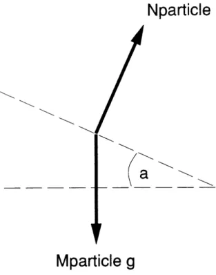
The free body diagram for the particle is slightly more complex since the direction of its acceleration in the fixed frame of reference is not entirely clear. Nevertheless, AMES has enough information to solve for this information. Figure 2.6.1 illustrates the free body diagram for the particle.

While it may not seem that AMES has enough information to solve for the normal force Npatide, it actually can. The acceleration of the particle in the fixed frame of

reference Apa,,tidec.fixed = Apa,.ticlu.wedge + Awedgecfized. This comes from AMES' reference frame conversion knowledge. It is useful since we know that Apartidc.,wedge is parallel to the top of the wedge, and we know that Awedge-cfived has magnitude

Nprti,, in and is directed leftward.

Mweoge

Nparticle

Mparticle g

Figure 2-12: Particle Free Body Diagram

Nparticle cos a - Mparticleg

Apartidectuedge

= - MpaticleAparticle+..wedge sin a

Mparticleg - Nparticle cos a

Mparticle sin a

In the vertical direction, by substituting in the above, AMES has:

Npatticle sin a = Mpartice (Aparticlewedge cos a - N sin a

Mparticle Npal

I(

Mwedge + Mpartidc sin2 a

Having solved for Npa,tidc, AMES can obtain each body's acceleration, velocity, and position versus time. Note that because Npartide > 0 for all time, the particle does not slip off the top of the wedge. The state therefore ends when either the