Discriminative training of acoustic models in a segment-based speech recognizer

-J

Discriminative Training of Acoustic Models in a

Segment-Based Speech Recognizer

by

Eric D. Sandness

S.B., Massachusetts Institute of Technology (2000)

Submitted to the Department of Electrical Engineering

and Computer Science

in partial fulfillment of the requirements for the degree of

Master of Engineering in Electrical Engineering and Computer Science

at the

MASSACHUSETTS INSTITUTE OF TECHNOLOGY

May 19, 2000

©

2000 Eric D. Sandness. All rights reserved.

The author hereby grants to MIT permission to reproduce and

distribute publicly paper and electronic copies of this thesis document

in whole or in part.

OF TECF JUL x

-- -BR

Author ...

Department of Electrical Engineering and Computer Science

lay 19, 2000

ENG

7 2000

Certified by ...

I. L

Hetherington

Research Scientist

ervisor

Accepted by...

Arthur C. Smit

Chairman, Departmental Committee on Graduate Students

Discriminative Training of Acoustic Models in a

Segment-Based Speech Recognizer

by

Eric D. Sandness

Submitted to the Department of Electrical Engineering and Computer Science on May 19, 2000, in partial fulfillment of the

requirements for the degree of

Master of Engineering in Electrical Engineering and Computer Science

Abstract

This thesis explores the use of discriminative training to improve acoustic modeling in a segment-based speech recognizer. In contrast with the more commonly used Maximum Likelihood training, discriminative training considers the likelihoods of competing classes when determining the parameters for a given class's model. Thus, discriminative training works directly to minimize the number of errors made in the recognition of the training data.

Several variants of discriminative training are implemented in the SUMMIT rec-ognizer, and these variants are compared using results in the Jupiter weather infor-mation domain. We adopt an utterance-level training procedure. The effects of using different training criteria, optimizing various model parameters, and using different values of training control parameters are investigated. Consistent with previous stud-ies, we find the most common objective criteria produce very similar results. We do, however, find that with our training scheme optimizing the mixture weights is much more effective than optimizing the Gaussian means and variances.

An extension to the standard discriminative training algorithms is developed which focuses on the recognition of certain keywords. The keywords are words that are most important for the proper parsing of an utterance by the natural language component of the system. We find that our technique can greatly improve the recog-nition word accuracy on this subset of the vocabulary. In addition, we find that choices of keyword lists which exclude certain unimportant, often poorly articulated words can actually result in an improvement in word accuracy for all words, not just

the keywords themselves.

The accuracy gains reported in this thesis are consistent with gains previously reported in the literature. Typical reductions in word error rate are in the range of

5% relative to Maximum Likelihood trained models.

Thesis Supervisor: I. Lee Hetherington Title: Research Scientist

Acknowledgments

I would first and foremost like to thank my thesis advisor, Lee Hetherington, for

his help throughout this project. He was always available to help me with whatever problems came up and he provided me with many insightful suggestions. I would also like to thank Victor Zue and the entire Spoken Language Systems group for making this a wonderful place to conduct research. This group has given me a great deal and

I appreciate it very much. I can not imagine a better place to have spent my time as

a graduate student.

Finally, I would like to thank everyone who has helped me to survive (somehow) my years at MIT. My friends here have made my collegiate experience a fun and memorable one. While I am thrilled to finally be done, I will also miss the good times

I have had at the Institute.

This research was supported by DARPA under contract DAANO2-98-K-0003, monitored through U.S. Army Natick Research, Development and Engineering Cen-ter; and contract N66001-99-8904, monitored through Naval Command, Control, and

Contents

1 Introduction to Discriminative Training 11

1.1 Introduction . . . . 11

1.2 Previous Research . . . . 12

1.3 Thesis Objectives . . . . 14

2 Experimental Framework 17 2.1 The Jupiter Domain . . . . 17

2.2 Overview of SUMMIT . . . . 19 2.2.1 Segmentation . . . . 20 2.2.2 Acoustic Modeling . . . . 21 2.2.3 Lexical Modeling . . . . 22 2.2.4 Language Modeling . . . . 22 2.2.5 The Search . . . . 23 2.2.6 Finite-State Transducers . . . . 23

2.3 The Acoustic Modeling Component . . . . 24

2.3.1 Acoustic Phonetic Models . . . . 24

2.3.2 Maximum-Likelihood Training . . . . 25

3 Gaussian Selection 27 3.1 Description of Gaussian Selection . . . . 27

3.1.1 M otivation . . . . 27

3.1.2 Algorithm Overview . . . . 28

3.2 Results in SUMMIT . . . . 29

3.3 Sum m ary . . . . 31

4 Implementing Discriminative Training in SUMMIT 33 4.1 Phone- Versus Utterance-Based Training . . . . 33

4.2 The Objective Function . . . . 35

4.2.1 The MCE Criterion . . . . 36

4.2.2 The MMI Criterion . . . . 38

4.3 Parameter Optimization . . . . 40

4.3.1 Adjusting the Mixture Weights . . . . 41

4.3.2 Adjusting the Means and Variances . . . . 42

4.4 Implementational Details . . . . 43

4.4.2 The Parameter Adjustment . . . . 4.4.3 Implementational Summary . . . . 4.5 Sum m ary . . . .

5 Discriminative Training Results

5.1 Results of Mixture Weight Training . . . .

5.1.1 MCE Training of the Mixture Weights . . . . 5.1.2 MMI Training of the Mixture Weights . . . . 5.2 Results of Training the Means and Variances . . . .

5.2.1 Altering One Dimension of the Means and Variances

5.2.2 Altering Only the Means . . . .

5.2.3 Limiting the Maximum Alteration Magnitude . . . 5.2.4 Increasing the Number of Dimensions Altered . . .

5.2.5 Summary and Conclusions . . . .

5.3 Sum m ary . . . .

6 Keyword-Based Discriminative Training

6.1 Hot Boundaries . . . .

6.2 Changes to the Training Procedure . . . .

6.3 A Training Experiment . . . .

6.4 Omission of Unimportant Words . . . .

6.5 Conclusions . . . .

7 Conclusion

7.1 Thesis Overview and Observations . . . . 7.2 Suggestions for Future Work . . . .

A Statistics File Format

B Lists of Words for Keyword Experiments B.1 Keywords for Keyword-Based Training . . B.2 Omitted Words for Omission Experiment .

44 46 47 49 . . . . 50 . . . . 50 . . . . 60 . . . . 69 . . . . . 69 . . . . 71 . . . . 73 . . . . 74 . . . . 75 . . . . 76 77 78 79 81 86 88 91 91 93 95 99 99 103

List of Figures

3-1 Test Set Accuracy vs. Gaussian Logprob Computation Fraction . . . 30 3-2 Test Set Accuracy vs. Overall Recognition Time Ratio . . . . 30

4-1 Comparison of cost functions of equations (4.3) and (4.4). Four com-peting hypotheses are used, whose scores are fixed at -549.0, -549.1,

-550.3, and -550.6. This is a typical score pattern that might be

ob-served for the top 4 hypotheses in an N-best list. p is set to 4.0. The curves are swept by varying the score of the correct hypothesis between -564.0 and -534.0. . . . . 38

4-2 Plot of MMI log likelihood function of equation (4.9), with and without a score threshold. As in figure 4-1, four competing hypotheses are used, whose scores are fixed at -549.0, -549.1, -550.3, and -550.6. T is set to 0.1. Again, the curves are swept by varying the score of the correct

hypothesis between -564.0 and -534.0. . . . . 40

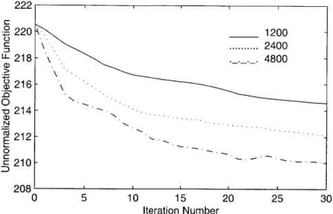
5-1 Change in Unnormalized Objective Function Value vs. Iteration Index

for MCE Weight Training, Base Case . . . . 51 5-2 Average Magnitude of the Weight Alterations vs. Iteration Index for

MCE Weight Training, Base Case . . . . 51 5-3 Sentence Accuracy on Development Data vs. Iteration Index for MCE

Weight Training, Base Case . . . . 52

5-4 Word Accuracy on test_500 vs. Iteration Index for MCE Weight Train-ing, B ase C ase . . . . 53 5-5 Unnormalized Objective Function vs. Iteration Index for MCE Weight

Training with Various Step Sizes . . . . 54

5-6 Word Accuracy on test_500 vs. Iteration Index for MCE Weight

Train-ing with Various Step Sizes . . . . 55 5-7 Maximum Weight Alteration Magnitude vs. Iteration Index for MCE

Weight Training with Various Rolloffs . . . . 56 5-8 Word Accuracy on test_500 vs. Iteration Index for MCE Weight

Train-ing with Various Rolloffs . . . . 57 5-9 Word Accuracy on test-500 vs. Iteration Index for MCE Weight

Train-ing with Various Numbers of CompetTrain-ing Hypotheses . . . . 58 5-10 Word Accuracy on test-500 vs. Iteration Index for MCE Weight

5-11 Change in Unnormalized Objective Function Value vs. Iteration Index

for MMI Weight Training, Base Case . . . . 61

5-12 Average Magnitude of the Weight Alterations vs. Iteration Index for MMI Weight Training, Base Case . . . . 62

5-13 Sentence Accuracy on Development Data vs. Iteration Index for MMI Weight Training, Base Case . . . . 63

5-14 Word Accuracy on test-500 vs. Iteration Index for MMI Weight Train-ing, B ase C ase . . . . 63

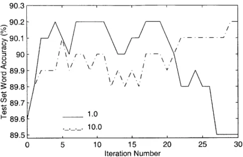
5-15 Word Accuracy on test-500 vs. Iteration Index for MMI Weight Train-ing with Various Step Sizes . . . . 64

5-16 Word Accuracy on test_500 vs. Iteration Index for MMI Weight Train-ing with Various Score Thresholds . . . . 66

5-17 Word Accuracy on test-500 vs. Iteration Index for MMI Weight Train-ing with Various Numbers of CompetTrain-ing Hypotheses . . . . 67

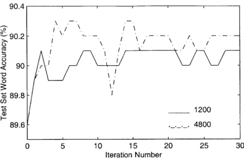
5-18 Word Accuracy on test-500 vs. Iteration Index for MMI Weight Train-ing usTrain-ing train_12000 . . . . 67

5-19 Change in Unnormalized Objective Function Value vs. Iteration Index for Mean/Variance Training, One Dimension . . . . 70

5-20 Sentence Accuracy on Development Data vs. Iteration Index for Mean/Variance Training, One Dimension . . . . 71

5-21 Word Accuracy on test-500 vs. Iteration Index for Mean/Variance Training, One Dimension . . . . 72

5-22 Word Accuracy on test_500 vs. Iteration Index for Means Only Train-ing, One Dim ension . . . . 72

5-23 Word Accuracy on test_500 vs. Iteration Index for Mean/Variance Training Without Maximum Alteration Limits, One Dimension . . . . 74

5-24 Word Accuracy on test_500 vs. Iteration Index for Mean/Variance Training, Three Dimensions . . . . 75

6-1 Examples of Choosing Hot Boundaries . . . . 79

6-2 New Score Computation Using Hot Boundaries . . . . 80

6-3 Typical Keywords . . . . 81

6-4 Change in Unnormalized Objective Function Value vs. Iteration Index for Keyword Training . . . . 82

6-5 Average Magnitude of the Weight Alterations vs. Iteration Index for Keyword Training . . . . 83

6-6 Keyword Accuracy on test_500 vs. Iteration Index for Keyword Training 84 6-7 Overall Word Accuracy on test_500 vs. Iteration Index for Keyword T raining . . . . 85

6-8 Overall Word Accuracy on test_500 vs. Iteration Index for Omitted W ords Training . . . . 87

List of Tables

2.1 Example of user dialogue with the Jupiter weather information system. 18 4.1 Word Accuracies for Preliminary Test Comparing Phone-Level and

Utterance-Level Criteria . . . . 35 5.1 Summary of Accuracies for MCE Weight Training with Various N-best

List Sizes and Training Set Sizes. . . . . 60 5.2 Summary of Accuracies for MMI Weight Training with Various N-best

List Sizes and Training Set Sizes. . . . . 68 6.1 Summary of Keyword Accuracies for Various Types of Training. . . . 83 6.2 Summary of Overall Word Accuracies for Various Types of Training. . 85 6.3 Overall Word Accuracies for Omitted Words Experiments Compared

Chapter 1

Introduction to Discriminative

Training

1.1

Introduction

Modern speech recognition systems typically work by modeling speech as a series of phonemes. These phonemes are described using some sort of probability density functions, often mixtures of multivariate Gaussian components. Various recogni-tion hypotheses are ranked by determining the likelihood of a set of input waveform measurements given the distributions of the hypothesized phonemes, combined with syllable and word sequence likelihoods imposed by the grammar of the language. The goal of the speech recognition process is to produce a transcription of the speaker's utterance with the minimum number of errors.

A major problem in building a successful speech recognition system is how to

find the likelihood functions for each sub-word class. Given a set of transcribed training data, a set of modeling parameters must be found which will minimize the number of recognition errors. The standard approach is to train the model parameters using Maximum-Likelihood (ML) estimation. This approach aims to maximize the probability of observing the training data for each class given that class's parameter estimates. However, maximizing this probability does not necessarily correspond to minimizing the number of misclassifications. ML estimation does not take the

likelihoods of incorrect classes into account during training, so potential confusions are ignored. Therefore, Maximum-Likelihood training does not always do a good job of discriminating near class boundaries.

Discriminative training aims to correct this deficiency by taking the likelihoods of potential confusing classes into account. Rather than trying to maximize the probability of observing the training data, it works to directly minimize the number of errors that are made in the recognition of the training data. More attention is given to data lying near the class boundaries, and the result is an improved ability to choose the correct class when the likelihood scores are close.

The goal of this thesis is to comparatively evaluate several discriminative training techniques in a segment-based speech recognition system. The next section provides an overview of previous research which serves as an introduction to some of the issues involved. Following that is a precise statement of the objectives of this thesis and an outline of the remaining chapters.

1.2

Previous Research

Much research has already been done on discriminative training of speech recognition parameters. Discriminative training procedures always employ an objective function which is optimized by some sort of update algorithm. The objective function should measure how well the current set of parameters classifies the training data. The update algorithm alters the system parameters to incrementally improve the objective score. The calculation of the objective function and subsequent alteration of the system parameters are repeated until the objective score converges to an optimum value.

The most common discriminative training criteria are Maximum Mutual Infor-mation (MMI) [21] and Minimum Classification Error (MCE) [7]. The basic aim of MMI estimation is to maximize the a posteriori probability of the training utterances given the training data, whereas MCE training aims to minimize the error rate on the training data. MMI focuses on the separation between the classes, while MCE

focuses on the positions of the decision boundaries.

The standard MMI objective function [27] encourages two different optimizations for each training sample: the probability of observing the sample given the correct model is increased, and the probabilities of observing the sample for all other models

are decreased. Classification errors will hopefully be corrected since the likelihood of the correct model for each sample is increased relative to the likelihoods of all other models. However, the amount of optimization is not dependent on the number of errors; even in the absence of classification errors on the training data significant optimization of the objective function can be performed. This is because MMI does not directly measure the number of classification errors on the training data, but rather the class separability.

By contrast, a wide variety of different objective functions are used for MCE

estimation. MCE objective functions measure an approximation of the error rate on the training data. While a simple zero-one cost function would of course measure this error rate perfectly, it is a piecewise constant function and therefore cannot easily be optimized by numerical search methods. A continuous approximation to the error rate must be used instead. Some simple objective functions (perceptron, selective squared distance, minimum squared error) are discussed in [16]. In most practical

MCE training procedures [7, 14, 16] a measure of misclassification is embedded into a smoothed zero-one cost function such as a translated sigmoid. Thus almost no penalty is incurred for data that is classified correctly, and data that is misclassified incurs a penalty that is essentially a count of classification error. MCE directly acts to correct classification errors on the training data; data that is classified correctly does not significantly influence the optimization process.

A comparison between the MMI and MCE criteria is done in [25]. It is shown

that both criteria can be mathematically expressed using a common formula. The criteria are found to produce similar results in practice.

The most common update algorithms used to iteratively alter the system pa-rameters are Generalized Probabilistic Decscent (GPD) and Extended Baum-Welch (EBW). GPD [6] is a standard gradient descent algorithm and is usually used to

optimize MCE objective functions. EBW

[13]

Many variations of discriminative training have been implemented and reported in the literature. Numerous combinations of parameters to optimize, optimization criteria, and recognition frameworks are possible. In [3] the mixture weights of a system based on Hidden Markov Models (HMMs) are optimized using MMI with sentence error rates. In [27], the means and variances of the HMM state distributions are adjusted using MMI. Corrective MMI training, a variation on MMI in which only incorrectly recognized sentences contribute to the objective function, is used in [19].

A less mathematically rigorous version of corrective training is used in [2] to optimize

HMM transition probabilities and output distributions. In [14], MCE training is used to compute means and variances of HMM state likelihoods. Relative reductions in word error rate of 5-20% compared to the same systems trained with the ML algorithm are typical.

Note that almost all of the previous research on discriminative training has been done using HMM-based recognition systems. By constrast, the research for this thesis will be performed using SUMMIT [10], a segment-based continuous speech recognition system developed by the Spoken Language Systems group at MIT. The opportunity to measure the effectiveness of discriminative training in a segment-based recognition framework is one of the original characteristics of the research that will be performed for this thesis.

1.3

Thesis Objectives

The principal goal of this thesis is to compare the effectiveness of various discrimina-tive training algorithms in a segment-based speech recognizer. While many previous experiments have utilized somewhat simple acoustic models (e.g., few classes or few

Gaussian components per mixture model) the experiments in this thesis will evalu-ate recognition performance using the full-scale SUMMIT recognizer in the medium-vocabulary Jupiter domain. This should provide a more realistic view of the acoustic modeling gains that may be possible in real speech recognition systems. The data from these experiments will allow a direct comparison of the effectiveness of MCE and MMI training. Also, the relative merits of altering different system parameters (i.e., mixture weights versus means and variances) can be compared. Finally, it will be possible to observe the effects of using different values for several training parameters, such as the step size and the number of hypotheses used for discrimination.

Another goal of this thesis is to extend the existing body of discriminative train-ing techniques for speech recognition. To this end a keyword-based discriminative training algorithm is developed. The goal of this technique is to shape the acoustic models to allow optimal recognition of the words that the system most needs in order to understand an utterance. This technique should reveal the extent to which the alteration of acoustic model parameters can be used to achieve specific recognition goals.

Chapter 2 describes the experimental framework for this thesis. The Jupiter domain is described and an overview of the SUMMIT speech recognizer is provided.

A detailed discussion of the acoustic modeling component of the recognizer is given.

Chapter 3 describes the technique of Gaussian Selection, which is used to reduce test set evaluation times in this thesis.

Chapter 4 discusses the details of the discriminative training algorithm. The objec-tive functions that will be used in this thesis are presented along with the algorithms used for parameter optimization. The implementation of discriminative training in SUMMIT is also discussed.

Chapter 5 presents results of various discriminative training experiments. Perfor-mance using both the MCE and MMI criteria for altering mixture weights, means and variances is evaluated.

Chapter 6 describes the new keyword-based discriminative training technique. Alterations to the standard discriminative training algorithm are introduced. Results

of some experiments are presented which show that the keyword-based technique actually produces the best results reported in this thesis using either a keyword-error rate metric or the overall word-error rate.

Finally, Chapter 7 summarizes the lessons of this thesis and presents some sug-gestions for future work in this area.

Chapter 2

Experimental Framework

This chapter contains background information for the experimental work presented in this thesis. First, the Jupiter weather information domain, which is used for all experiments in this thesis, is discussed. Next, an overview of the SUMMIT speech recognition system is presented that illustrates how the acoustic modeling component fits into the recognizer as a whole. Finally, the acoustic modeling component is described in more detail.

2.1

The Jupiter Domain

Recognition experiments were performed using the corpus associated with the Jupiter telephone-based weather information system [30]. Users can call and receive weather information from various online sources over the phone. Jupiter has information on approximately 500 cities, 60% of them in the United States. The system can provide weather reports for a given day or for a period of several days. It can also answer specific questions about such weather phenomena as temperature, wind speed, precipitation, sunrise and sunset times, pressure, and humidity. An example dialogue between Jupiter and a real user is given in Table 2.1.

The Jupiter corpus contains quite a realistic body of data. Jupiter has a medium vocabulary of 1957 words, of which nearly half are geography-related words. The spoken utterances come mostly from calls to a toll-free number; almost all of these

Jupiter: Hi! Welcome to Jupiter, the MIT Lab for Computer Science

weather information system. This call is being recorded for system development. You may hang up or ask for help at any time. How can I help you?

User: Can you tell me what's the weather like in Boston today?

Jupiter: In Boston this afternoon. Partly sunny early. Then becoming cloudy with 30 percent chance of showers toward evening. Tonight: rain. Possibly heavy at times. Near 100 percent chance of rain. Can I help you with something else? User: Yes what about San Francisco?

Jupiter: In San Francisco today: patchy fog near the ocean morning.

Otherwise mostly sunny. Tonight: areas of coastal fog and low clouds. Otherwise fair. Is there something else I can do for you?

User: Yes, how cold is it in Dallas Texas today?

Jupiter: In Dallas today: high upper 40s. Tonight: lows near 32. What else would you like to know?

User: I'd like to know whether it's snowing in Detroit.

Jupiter: I'm sorry, I didn't understand you. Please rephrase your query. User: What is the weather in Detroit?

Jupiter: In Detroit this afternoon: occasional light rain and drizzle. Tonight: rain showers likely. Becoming snow showers by late tonight. 70 percent chance of precipitation.

Table 2.1: Example of user dialogue with the Jupiter weather information system.

consist of spontaneous speech from untrained or self-trained users. Only spontaneous, in-vocabulary utterances are used for training in this thesis.

In this thesis, three sets of training data are used. The first, train_6000, is used for the majority of experiments with traditional discriminative training and contains 6000 utterances. The second, train_12000, is used for comparative purposes and contains 12000 utterances. The third, train_18000, contains about 18000 utterances and is only used for the keyword-based training experiments in Chapter 6. During training, the training sets are subdivided into two functional groups: eighty percent of the data is used for training, and twenty percent is set aside for development evaluations.

Two test sets are used. The first, test_500, is used for the majority of recognition experiments and contains 500 in-vocabulary utterances. For the more successful ex-periments, performance is further measured using the 2500 utterance set test-2500, which contains a full sampling of in-vocabulary and out-of-vocabulary utterances.

2.2

Overview of SUMMIT

SUMMIT is a segment-based continuous speech recognition system developed at MIT [10]. This type of recognizer attempts to segment the waveform into predefined

sub-word units, such as phones, sequences of phones, or parts of phones. Frame-based recognizers, on the other hand, divide the waveform into equal-length windows, or frames [23]. The first step in either approach is to extract acoustic features at small, regular intervals. However, segment-based approaches next attempt to segment the waveform using these features, while frame-based recognizers use the frame-based features directly.

The result of the segmentation is a sequence of hypothesized segments together with their hypothesized boundaries. As discussed in section 2.2.2, the signal can either be represented with measurements taken inside the segments or measure-ments centered around the boundaries. In this thesis, only boundary-based mea-surements are used. Thus the recognizer must take a set of acoustic feature vectors

A = {-, a-' , -- , _{a7v}, where N is the number of hypothesized boundaries, and find}

the most likely string of words z* = {w1, w2, - - , WM} that produced the waveform.

In other words,

= arg max Pr(Z|A) (2.1) where w' ranges over all possible word strings. Each word string may be realizable as different strings of units UT with different segmentations s, but since all hypotheses are evaluated on the same set of boundaries when using boundary-based measurements, the likelihood of s need not be considered when comparing the likelihoods of different word strings. Thus equation (2.1) becomes:

*= argmaxYPr(-,ZIA) (2.2) where u' ranges over all possible pronunciations of '. To reduce computation SUM-MIT assumes that, given a word sequence ', there is an optimal unit sequence which is much more likely than any other U'. This replaces the summation by a maximization

in which we attempt to find the best combination of word string and unit sequence given the acoustic features:

arg maxPr( i, iiA) (2.3)

Applying Bayes' Rule, this can be rewritten as:

Pr(A t', i') Pr(tJt') Pr(')

{ ,* = arg max (2.4) w,u Pr(A)

=argma~x Pr(Alw', 5) Pr(u'lw) Pr(w') (2.5)

The division by Pr(A) can be omitted since Pr(A) is constant for all W' and U' and therefore does not affect the maximization.

The estimation of the three components of the last equation is performed by, respectively, the acoustic, lexical, and language modeling components. The following four sections briefly describe the major components of the recognizer: segmentation, acoustic modeling, lexical modeling, and language modeling. Afterwards we describe how SUMMIT searches for the best path and the implementation of SUMMIT using finite-state transducers.

2.2.1 Segmentation

The essential element of the segment-based approach is the use of explicit segmental start and end times in the extraction of acoustic measurements from the speech signal. In order to implement this measurement extraction strategy, segmentation hypotheses are needed. In SUMMIT, this is done by first extracting frame-based acoustic features (e.g., MFCC's) at small, regular intervals, as in a frame-based recognizer. Next, boundaries between segments must be hypothesized based on these features. There are various ways to perform this task. One method is to place segment boundaries at points where the rate of change of the spectral features reaches a local maximum; this is called acoustic segmentation [9]. Another method, called probabilistic segmentation

acoustic segmentation is used.

2.2.2

Acoustic Modeling

There are two types of acoustic models that may be used in SUMMIT: segment models and boundary models [26]. Segment models are intended to model hypothesized phonetic segments in a phonetic graph. The observation vector is typically derived from spectral vectors spanning the segment. Segment-based measurements from a hypothesized segment network lead to a network of observations. For every path through the network, some segments are on the path and others are off the path. When comparing different paths it is necessary for the scoring computation to account for all observations by including both on-path and off-path segments in the calculation

[5, 11].

In contrast, boundary models are intended to model transistions between phonetic units. These are diphone models with observation vectors centered at hypothesized boundary locations. Some of these landmarks will in reality be internal to a phone, so both internal and transition boundary models are used. Every path through the net-work incorporates all of the boundaries through either internal or transition boundary models, so the scores for different paths can be directly compared.

Boundary models are used exclusively in this thesis for two reasons. First, since every recognition hypothesis is based on the same set of measurement vectors, col-lecting statistics for discriminative training is much easier. Second, performance in Jupiter has been shown to be better using boundary models than when using independent segment models [26]. With considerably more computation, context-dependent triphone segment models can improve performance further.

SUMMIT assumes that boundaries are independent of each other and of the word string, so that

N

Pr(Ajzi, iI) = flPr(dajbi) (2.6)

where b, is the lth boundary label as defined by U'. During recognition, the acoustic model assigns to each boundary in the segmentation graph a vector of scores

corre-sponding to the probability of observing the boundary's features given each of the boundary labels. In practice, however, only the scores that are being considered in the recognition search are actually computed.

The details of how the likelihoods of a given measurement vector are computed for each boundary label are presented in section 2.3.

2.2.3

Lexical Modeling

Lexical modeling is the modeling of the allowable pronunciations for each word in the recognizer's vocabulary [29]. A dictionary of pronunciations, called the lexicon, contains one or more basic pronunciations for each word. In addition, alternate pronunciations may be created by applying phonological rules to the basic forms. The alternate pronunciations are represented as a graph, the arcs of which can be weighted to account for the different probabilities of the alternate pronunciations. The probability of a given path in the lexicon accounts for the lexical probability component in (2.5).

2.2.4

Language Modeling

The purpose of the language model is to determine the likelihood of a word sequence

w. Since it is usually infeasible to consider the probability of observing the entire

sequence of words together, n-grams are often used to consider the likelihoods of observing smaller strings of words within the sequence

[1].

N

Pr() =

JJ

where N is the number of words in '. The probability estimates for n-gram language models are usually trained by counting the number of occurrences of each n-word sequence in a set of training data, although smoothing methods are often needed to redistribute some of the probability from observed n-grams to unobserved n-grams.

In all of the experiments in this thesis, bigram and trigram models (n=-2 and 3, respectively) are used.

2.2.5

The Search

Together, the acoustic, lexical, and language model scores form a weighted graph representing the search space. The recognizer uses a Viterbi search to find the best-scoring path through this graph. Beam-pruning is used to reduce the amount of computation required. In the version of SUMMIT used in this thesis, the forward Viterbi search uses a bigram language model to obtain the partial-path scores to each node. This is followed by a backward A* beam search using the scores from the Viterbi search as the look-ahead function. Since the Viterbi search has already pruned away much of the search space, a more computationally demanding trigram language model is used for the backward A* search. This produces the final N-best recognition hypotheses.

2.2.6

Finite-State Transducers

The recognition experiments in this thesis utilized an implementation of SUMMIT using weighted finite-state transducers, or FSTs [12]. The FST recognizer R can be represented as the composition of four FSTs,

R = A o D o L o G (2.8)

where A is a segment graph with associated acoustic model scores, D performs the conversion from the diphone labels in the acoustic graph to the phone labels in the lexicon, L represents the lexicon, and G represents the language model. Recognition then becomes a search for the best path through R. The composition of D, L, and

G can be performed either during or prior to recognition. In this thesis D o L o G is

computed as D o min(det(L o G)), and the composition with A occurs as part of the Viterbi search.

2.3

The Acoustic Modeling Component

As seen in the previous section, the job of the acoustic modeling component of the recognizer is to compute Pr(AJWY, i'). This reduces to a product of individual terms of the form Pr(d'ilbi), where b, is the lth boundary label defined by U'. This section describes how the probability density functions for each boundary label are modeled,

and how the model parameters are trained given a set of training data.

2.3.1

Acoustic Phonetic Models

Acoustic phonetic models are probability density functions over the space of possible measurement vectors, conditioned on the identity of the phonetic unit. Normalization and principal components analysis are performed on the measurement vectors prior to modeling. Then the whitened vectors are modeled using mixtures of diagonal

Gaussian models, of the following form:

M

p(V|u) = Wipi(|U) (2.9)

where M is the number of mixture components in the model, a is a measurement vector, and u is the unit being modeled. Each pi(d) is a multivariate normal prob-ability density function with no off-diagonal covariance terms, whose value is scaled

by a weight wi. The mixture weights must satisfy

M

Ewi = 1 (2.10)

i=1

0 <w i < 1 (2.11)

Thus the parameters used to model a given phonetic unit are M weights, Md means, and Md variances, where d is the dimensionality of the whitened measurement vector. The score of an acoustic model is the value of the mixture density function at the given measurement vector. For practical reasons, the logarithm of this score is used during computation, resulting in what is known as the log likelihood score for the

given measurement vector.

2.3.2

Maximum-Likelihood Training

Before the Gaussian mixture models can be trained, a time-aligned phonetic tran-scription of each of the training utterances is needed. These are automically gener-ated from manual word transcriptions using forced phonetic transcriptions, or forced paths. Beginning with a set of existing acoustic models, we perform recognition on each training utterance using the known word transcription as the language model. Next, the principal components analysis coefficients are trained from the resulting measurement vectors, producing a set of labeled 50-dimensional vectors. The data are separated into different sets corresponding to each lexical unit.

Training a Gaussian mixture model for a given unit is a two-step process. In the first step, the K-means algorithm [8] is used to produce an initial clustering of the data. In this thesis the number of clusters generated (i.e., the number of mixture components) is either 50 or the number possible with at least 50 training tokens per cluster, whichever is smaller. This ensures that each mixture component is trained from sufficient data. In the second step, the results of the K-means algorithm are used to initialize the Expectation-Maximization (EM) algorithm [8]. The EM algorithm iteratively maximizes the likelihood of the training data and estimates the parameters of the mixture distribution. It converges to a local maximum; there is no guarantee of achieving the global optimum. The outcome is dependent on the initial conditions obtained from the K-means algorithm.

The result of the training is a set of model parameters which maximizes the likelihood of observing each class's training data given the parameters. Note that only the training data belonging to a given class affects that class's parameter estimates. Discriminative training aims to incorporate additional knowledge by also using the data associated with potential confusing classes.

Chapter 3

Gaussian Selection

This chapter discusses the technique of Gaussian Selection [4, 18]. First, the motiva-tion for using Gaussian Selecmotiva-tion and mathematical formulamotiva-tion of the technique are presented. Next, the results of applying Gaussian Selection to the acoustic models in

SUMMIT are discussed. Finally, the most important features of Gaussian Selection

are summarized.

3.1

Description of Gaussian Selection

Gaussian Selection is a technique which reduces the time required to estimate acoustic likelihood scores from Gaussian mixture models. This section discusses the motivation for using this technique and the details of its implementation.

3.1.1

Motivation

In a real-time conversational system such as Jupiter, not only the accuracy but also

the computational requirements of the acoustic models are critical. Overall, up to

75% of the recognizer's time is spent evaluating the likelihoods of individual Gaussians

in the various Gaussian mixture models. Thus it is necessary to keep the number of Gaussians evaluated as low as possible in order to perform recognition in real time. Previously, techniques such as beam pruning during the Viterbi search have been

used to reduce the number of scores that need to be computed, but these techniques result in a large degradation in recognition accuracy. We need to find a way to prune away computations that do not have much effect on recognition accuracy.

In practice, the majority of the individual Gaussian likelihoods are completely negligible. The total likelihood score for a Gaussian mixture model is the sum of these individual likelihoods. There are usually a few Gaussians which are "close" to a given measurement vector and have much higher likelihoods than the rest of the Gaussians. Thus, the score for the mixture is approximately equal to the sum of the these few likelihoods. The likelihoods for the rest of the Gaussians do not need to be computed to maintain a high degree of accuracy in the overall score.

The motivation behind Gaussian Selection is to efficiently select the mixture com-ponents that are close to a given measurement vector, so that only the likelihoods for these Gaussians must be computed. The algorithm for accomplishing this is described next.

3.1.2

Algorithm Overview

To evaluate a model, the feature vector is quantized using binary vector quantization, and the resulting codeword is used to look up a list of Gaussians to evaluate. The lists of Gaussians to be evaluated for each model m and codeword k are computed beforehand.

A Gaussian is placed in the shortlist for a given m and k if the distance from its

mean to the codeword center is below some threshold

.

E (mi(d) - Ck(d)) <

e

Dd=1

There are two other ways a Gaussian can be placed in shortlist (M, k). A Gaussian is automatically placed in the list if its mean quantizes to k. This means that every Gaussian will be selected for at least one codeword. If m has no Gaussians associated

with k based on the above criteria, the closest Gaussian is placed in the list. This ensures that at least one Gaussian will be evaluated for every model/codeword pair, preserving a reasonable amount of modeling accuracy.

During model evaluation likelihood scores are computed for the Gaussians at each of the indices specified in the shortlist. Only these scores are combined to produce the total likelihood score for the model.

3.2

Results in SUMMIT

The effectiveness of Gaussian Selection was evaluated in Jupiter. Two similar metrics of computational load were used. The first metric is the computation fraction as defined in [4] and [18]:

C = Nnew +VQcomp (3.2)

where New and Nfull are the average number of Gaussians evaluated per feature

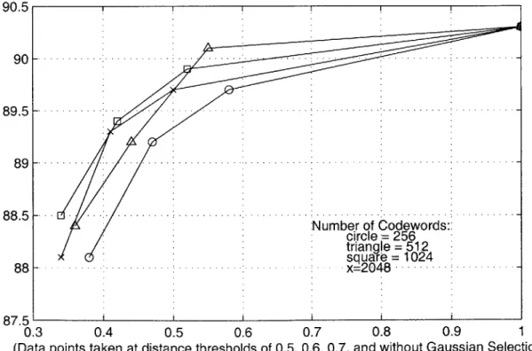
vector in the systems with and without Gaussian Selection, respectively, and VQcomp is the number of computations required to quantize the feature vector. The second metric is a ratio of the overall recognition times with and without Gaussian Selection. Word accuracy in Jupiter is plotted against these metrics in figures 3-1 and 3-2. Curves are plotted for codebook sizes of 256, 512, 1024, and 2048. Each curve is swept out by varying the distance threshold E. The data for these curves was collected running the recognizer on a set of 500 test utterances.

As can be observed from the figures, very little recognition accuracy is lost for values of E down to 0.7. Lowering 0 further causes accuracy to degrade quite rapidly. Performance does not appear to be terribly sensitive to the choice of codebook size.

At the optimum point for this data (512 codewords, 0 = 0.7), a 67% reduction

in Gaussian evaluations results in an overall reduction of recognition time of 45%, a speedup by a factor of 1.8. Thus it is obvious that reducing computation in the acoustic modeling component has a large, direct impact on the speed of the recognizer, with little degradation of accuracy.

90.5 90 F 89.5 F 89 I-88.5 1-88 F 87.5L-0.1

(Data points taken at distance thresholds of 0.5, 0.6, 0.7, and without Gaussian Selection)

Figure 3-1: Test Set Accuracy vs. Gaussian Logprob Computation Fraction

Number of Codewords: circle = 256 triangle =512 square= 1024 -. .. - - .x=2048 .... -0.3 0.4 0.5 0.6 0.7 0.8 0.9 1

(Data points taken at distance thresholds of 0.5, 0.6, 0.7, and without Gaussian Selection)

Figure 3-2: Test Set Accuracy vs. Overall Recognition Time Ratio 90.5 901 89.51 89 88.51 881 07.5 Number of Codewords: circle = 256 triangle = 512 square = 1024 x=2048 -0.2 0.3 0.4 0.5 0.6 0.7 0.8 0.9 1

these did not offer any advantages in our system. We also tried using a Gaussian log probability in place of squared distance without noticing any improvement. Finally, we tried limiting the size of the shortlists as in [181, but this did not improve upon the speed/accuracy tradeoff [26].

3.3

Summary

This chapter discussed the technique of Gaussian Selection. By vector quantizing the feature vector and only evaluating Gaussians which are within some distance threshold from the codeword center, the computation required to score acoustic models can be greatly reduced. In SUMMIT, we found that the overall recognition time can be decreased by 45% with a very small decrease in word accuracy.

Gaussian Selection has now been incorporated into the mainstream SUMMIT recognizer; for an example of how it is used see [26]. Since this thesis aims to use the most realistic recognition conditions possible, Gaussian Selection is used in all recognition experiments. One major reason for discussing Gaussian Selection here is to emphasize that this introduces a small amount of extra uncertainty in the test set accuracies. For example, a gain obtained from altering the acoustic models may be at least partially accounted for by a coincidental decrease in errors caused by Gaussian Selection in the new acoustic space. However, we have seen that Gaussian Selection is not terribly sensitive to the exact values of the parameters in the models; thus, for the incremental changes used in discriminative training, the extra uncertainty in comparing accuracies should be quite small.

Chapter 4

Implementing Discriminative

Training in SUMMIT

This chapter discusses the procedures used for discriminative training in this thesis. The training process requires a body of training data, an objective function, and a parameter optimization method. The training data is first scored using the current classifier parameters. The objective function then takes in these scores and provides a measure of classification performance. The parameter optimization method provides a way to alter the chosen parameters in order to maximize or minimize the objective function. If the objective function is a good measure of classifier accuracy, then optimizing it will minimize the number of recognition errors made. The first section describes two different ways of dividing up the training data and computing scores to be fed into the objective function. The next two sections describe the objective functions and parameter optimization formulas used in this thesis. Finally, we give an overview of the implementation of the training process as a collection of routines in SUMMIT.

4.1

Phone- Versus Utterance-Based Training

The first decision that must be made is how to divide up the training data into func-tional units that can be scored using the classifier parameters. The two possibilities

considered here are the use of phone-level scores and the use of utterance-level scores.

If a phone-level discriminative criterion is to be used, the training data is broken

down into a set of labeled phonemes. Each observation vector is sorted into a group based on its assigned label. The scores to be fed into the objective function are the pure classifier scores for each observation vector. The correct score is the score for the model corresponding to the vector's label, and the competing scores are the scores for all of the other models. This criterion attempts to maximize the acoustic score of the correct phone model for each observation vector independent of the context from which it was derived.

With an utterance-level discriminative criterion, on the other hand, the training data is organized into utterances. Each utterance consists of a sequence of observation vectors. The scores to be fed into the objective function are the complete recognizer scores for each utterance, i.e., the sum of the acoustic, lexical, and language model scores. The correct score is the recognition score for the actual spoken utterance, and the competing scores are the scores for all other possible utterances. Of course, it is not practical to train against every possible utterance, so an N-best list of competing utterances is used. This criterion attempts to adjust the acoustic models to maximize the chances of the correct utterance hypothesis being chosen, taking into account the effects of the non-acoustic components of the recognizer.

Some preliminary tests were run using several of the objective functions and op-timization methods to be discussed in the next two sections. While phone-level dis-criminative training decreased the number of classification errors made on unseen observation vectors, it actually increased word error rates when the updated acous-tic models were incorporated into the recognizer. We believe this to be due to the fact that the assignment of the correct label to a given boundary does not necessar-ily occur when ge - gh > 0, where g, and gh are the acoustic scores for the correct

and best competing models, respectively. Instead, proper assignment occurs when

9, - gh > E, where E is some threshold determined by the relative non-acoustic

scores of the hypotheses differing only at that boundary. In fact, E can be -oc if linguistic constraints make the competing label impossible at the boundary. Thus,

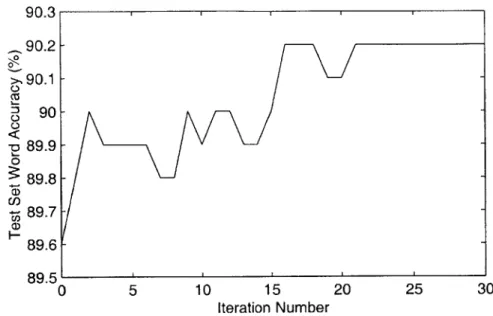
Models Word Accuracy ML Models 89.6

Phone-Level Training 89.2

Utterance-Level Training 90.2

Table 4.1: Word Accuracies for Preliminary Test Comparing Phone-Level and Utterance-Level Criteria

phone-level discriminative training can make many alterations that do not improve the recognizer and, in fact, may degrade its accuracy. Utterance-level discriminative training, which takes non-acoustic scores into consideration when altering the acous-tic parameters, improved both classifier performance and the word accuracy of the recognizer. In light of this, utterance-level scores were chosen for use in this thesis.

Table 4.1 gives word accuracies from one of the preliminary tests illustrating the superiority of the utterance-level criterion. These accuracies were obtained training the mixture weights with an MCE objective function (to be discussed in the next section). Exactly ten training iterations were performed, and the resulting models were evaluated using the test-500 set. Clearly, training with a phone-level criterion has a negative impact on word accuracy, while the utterance-level criterion produces the desired effect.

Thus, one set of scores is passed to the objective function for each utterance: the combined recognition score for the correct hypothesis, and recognition scores for the

N hypotheses in some N-best list. This set of scores is very similar to that which

was used for sentence-level training in [3].

4.2

The Objective Function

A variety of different objective functions are possible in discriminative training. There

are two primary characteristics that are desirable in any choice of objective function. First, as the function's value is improved, the classifier performance should also im-prove. Second, it should be continuous in the parameters to be optimized so that numerical search methods can be employed. Most discriminative training algorithms

reported in the literature use a variant on one of two broad classes of objective func-tions: a Minimum Classification Error (MCE) discriminant or a Maximum Mutual Information (MMI) discriminant. Descriptions of these classes of objective functions as well as the particular realizations that are used in this thesis are given next.

4.2.1

The MCE Criterion

A large variety of different objective functions are classified into the category of MCE

discriminants. The defining characteristic of this group is that the functions are designed to approximate an error rate on the training data. A simple zero-one cost function would measure this error rate perfectly, but it violates the constraint that the function should be continuously differentiable in the classifier parameters. As noted in Chapter 1, most practical MCE training procedures in the literature use a measure of misclassification embedded into a smoothed zero-one cost function. An example of a common misclassification measure [16] is:

1

1Nh,,, 7 7

ds(X,, A) = -gc,8(Xs, A) + E gh, (Xs, A (4.1)

Nh,s h=1I

where X. denotes the sequence of acoustic observation vectors for the sentence, A represents the classifier parameters, gc,, is the log recognizer score for the sentence's

correct word string, gh,s is a log recognizer score for a competing hypothesis, and Nh,S

is the number of competing hypothesis in the sentence's N-best list. From this point forward ge,s, gh,s, and Nh,s are shortened to g,, gh, and Nh for notational convenience, but it should be remembered that these are all different for every sentence. r is a positive number whose value controls the degree to which each of the competing hypothesis is taken into account.

This misclassification measure can be embedded in a number of smoothed zero-one cost functions. In this thesis we choose:

1

where p is the rolloff, which defines how sharply the function changes at the transition point, and a defines the location of the transition point. In this thesis a is always set to zero. The contribution of each utterance to the total objective score is given by

fS.

It turns out that the misclassification measure of Equation (4.1) is not very sensi-tive to the value of q for the numbers we use. For simplicity, then, rJ is set to 1. After

moving the g, term inside the sum and substituting the new formula for ds into the equation for

f

1

fS

1 + ek Nh((X,A)-(X,A))

Equation (4.3) is still just the cost function of [16], with q set to 1 and a set to 0. We decided to experiment with another equation similar to (4.3), but with the sum over competing hypotheses done outside instead of inside the sigmoid:

1 Nh ₁

fS(X, A) = _ 1 + eP(gc(XsA)-gh(Xs,A)) _(4.4)

This function still ranges from 0 to 1, but it allows each competing hypothesis to make a more individual contribution to the value. In the limiting case as p -+ oc, the function in Equation (4.3) can only take on two distinct values (0 and 1), but the function in Equation (4.4) can take on (Nh + 1) different values (-L, 0 < k < Nh).

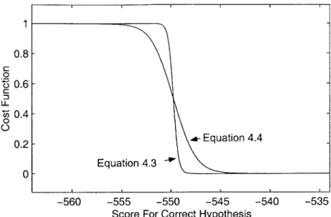
For moderate values of p, however, equations (4.3) and (4.4) produce very similar behaviors. This is illustrated in figure 4-1, which traces the curves of (4.3) and (4.4) with typical values for the competing scores. The only difference between the two curves is that the one defined by (4.4) transitions a bit more slowly. We choose to use the form in (4.4) since it is easier to calculate the derivative when the sum is on the outside.

To get the complete objective function, the cost functions of all of the training utterances are averaged together. Thus, the formula for the MCE objective function

1 0.8 0.6 F - Equati ation 4.3 --545 ion 4.4 -540 0.4 -0.2 -Equ -560 -555 -550 0 -535

Score For Correct Hvoothesis

Figure 4-1: Comparison of cost functions of equations (4.3) and (4.4). Four competing hypotheses are used, whose scores are fixed at -549.0, -549.1, -550.3, and -550.6. This is a typical score pattern that might be observed for the top 4 hypotheses in an N-best list. p is set to 4.0. The curves are swept by varying the score of the correct hypothesis between -564.0 and -534.0.

is: TMCE (A) 1 N, NEZf(X,,A) Ns S=1 1 N8 N- _{I E} Nh ₁ N_ 1 + eP(9c(xSA)-9h(X,A))

where N, is the total number of training utterances. This is the function we will use for MCE training experiments in this thesis.

4.2.2

The MMI Criterion

Unlike the MCE case, the MMI criterion comes with one standard objective function

[27]. In place of a cost function to be minimized, there is a likelihood ratio to be

maximized. This ratio is given by:

f,(X,, A) = log PC(X,, A) X, A) + E=h Iph(Xs, A) 0: 0 (4.5) (4.6) (4.7)

where pc and the Ph's are the linear versions of the recognizer scores, i.e.:

gh (X,, A) = log ph(X5, A) (4.8)

The log is used in the likelihood ratio to avoid computing with very small numbers. In terms of the log likelihood scores that the recognizer actually produces, (4.7) can be rewritten as:

Nh

fs(X, A) = ge(X, A) - Iog(ec(XsA) + E e"h(Xs,^)) (4.9)

h=1

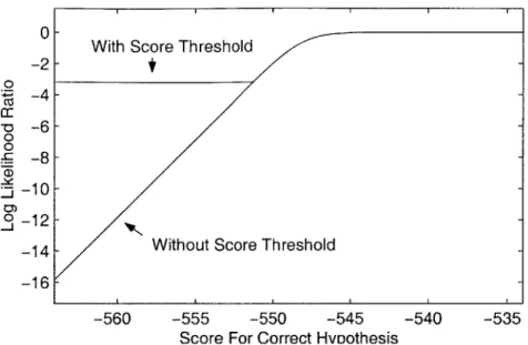
In order to compare the behavior of f, in the MMI criterion with the behavior of f, in the MCE criterion, figure 4-2 shows f. plotted as a function of g, for the same compet-ing hypotheses as in figure 4-1. As can be seen in the figure, f, is approximately linear up to the point when the correct score is slightly greater than the best competing score. At this point f, levels off and asymptotically approaches 0. Note that because of the logarithm, there is no lower bound on f,, which implies two things. First, f, can vary over a much larger range than

f,

f. can still have a significant derivative with respect to changes in parameter values.

Thus MMI will encourage optimizations to improve very poorly scoring utterances, in contrast to MCE which is relatively insensitive to these utterances. This can have a negative effect on error rates if these optimizations never improve the targeted ut-terances enough to actually correct any errors, while at the same time detracting from optimizations meant to improve more typical utterances. In order to keep MMI training from encouraging these optimizations, a score threshold T can be introduced.

The highest score among the correct and competing hypotheses is the best score. Any

of the other scores for which Ph < Tpbest are treated as if they were Tpbest. In other

words, a floor is placed on the score values. When small changes are made to these score values, they will still be treated as TPbest, and thus the objective score will no longer be sensitive to very poorly scoring hypotheses. Figure 4-2 also shows the behavior of f, when a score threshold is used.