Distance Estimation Through Wavefront Curvature In Cellular Systems
by
Geoffrey M. Gelman
Submitted to the Department of Electrical Engineering and Computer Science
in Partial Fulfillment of the Requirements for the Degrees of
Bachelor of Science in Electrical Science and Engineering
and Master of Engineering in Electrical Engineering and Computer Science
at the Massachusetts Institute of Technology
May 21, 1999
Copyright 1999 Geoffrey M. Gelman. Aliights reserved.
The author hereby grants to M.I.T. permission to reproduce and distribute publicly paper and electronic copies of this thesis
and to grant to others the right to do so.
Author
Department of/Electrical Engineering and
omputer
Science May 21, 1999 Certified by Dr. Vincent Chan2
o-e'is Supervisor Accepted by ______________________ Arthur C. Smith Chairman, Department Committee on Graduate ThesesDistance Estimation Through Wavefront Curvature In Cellular Systems
by
Geoffrey M. Gelman
Submitted to the
Department of Electrical Engineering and Computer Science
May 21, 1999
In Partial Fulfillment of the Requirements for the Degree of Bachelor of Science in Electrical Science and Engineering
and Master of Engineering in Electrical Engineering and Computer Science
Abstract
An urban environment presents difficulties in locating the source of a cellular signal using an antenna array receiver. A signal often travels over several "multipaths" involving reflection and diffraction before arriving at the receiver. Using information available in the arriving signal copies, certain paths may be selected as providing the most accurate informa-tion about the source's locainforma-tion. The deviainforma-tion of an arriving signal's wavefront from that of a plane wave provides information about the sig-nal source's range. Under certain conditions involving a wide aperture antenna, this range may be roughly estimated in order to help choose amongst signal multipaths. Furthermore, this estimation may be per-formed in a computationally efficient manner.
Thesis Supervisor: Vincent Chan
Contents
1 Introduction2 Background
2.1 Direction Finding Algorithms . . . .
2.2 Generalized Beamformers . . . .
2.3 Electro-magnetics . . . . 2.4 Geometrical Optics and the Geometric Theory of
2.5 The Sparse Array . . . . 2.6 Array Errors . . . . Diffraction 3 Cramer-Rao Bounds 3.1 D efinitions . . . . 3.2 D erivations . . . . 4 Methods 4.1 Softw are . . . . 4.2 A Typical Simulation. . . . . 5 Simulation Experiments
5.1 Obtaining a Precise Angle Estimate . . . . 5.2 Separating Range and Angle Searches . . . . 5.3 Accuracy of Range and Angle Estimators . . . . 5.4 Filled A rray . . . .
5.5 Small Aperture Array . . . . 10
6 Results 47
6.1 Obtaining a Precise Angle Estimate . . . . 47
6.2 Separating Range and Angle Estimates . . . . 51
6.3 Accuracy of Range and Angle Estimators . . . . 51
6.4 Filled A rray . . . . 58
6.5 Small Aperture Array . . . . 58
7 Discussion 62
8 Acknowledgments 67
A Proof that Maxima in S Plots are Isolated 68
List of Figures
1 An urban phone call. . . . . 11
2 Decreasing curvature of a wavefront with distance. . . . . 12
3 Plane wave incident on an antenna array. . . . . 14
4 The diffraction of a plane wave about a half-plane. . . . . 21
5 The diffraction of a plane wave about a half-plane, based on the analytic solution. The half-plane is located along the positive x ax is. . . . . 22
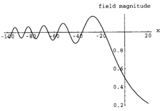
6 Field magnitudes according to the analytic solution. These mag-nitudes were plotted over the contour, y = -1000A. Negative val-ues of x correspond to the bright region of the half-plane, while positive values of x correspond to the shadow region. . . . . 24
7 Field magnitudes according to geometrical optics, before diffraction. 24 8 The physical meaning of the symbols used in the bound derivation. 29 9 Bounds on the standard deviation of range estimators for SNR of 10, 20, and 30dB, plotted at 0 = 0. The top curve is for 10dB. The bottom is for 30dB. Axes units are in A. . . . . 35
10 Bounds on the standard deviation of a range estimator plotted at ranges of 667A, 3333A, and 6667A (100m, 500m, and 1000m). The top curve is for 6667A. The bottom curve is for 667A. SNR is 20dB. Horizontal axis units are radians. Vertical axis units are A. ... ... 36
11 Bounds on the standard deviation of a range estimator plotted at 0 = 0. The top curve is the bound for a small aperture array, while the bottom is the curve for the sparse array. Axes units are
A... ... 36 12 S statistic plot for a half-plane source location at (r, 0) = (667A, -}) =
(loom, -i). Axes units are in A. . . . . 40
13 S statistic plot for a half-plane source location at (r, 0) = (667A, -i) =
(loom, -i). Axes units are in A. . . . . 41
14 S statistic plot for a half-plane source location at (r, 0) = (3333A, -6) = (500m, -i). Axes units are in A. . . . . 41
15 S statistic plot for a half-plane source location at (r, 0) = (667A,
})
=(loom, L). Axes units are in A. . . . . 42
16 Antenna arrays in the bright and shadow regions of a half-plane trying to locate a transmitter. . . . . 42
17 Source locations for testing the beamformer. Note that the black dots represent the edges of a half-plane, not point sources. . . . . 44
18 Angle estimate as a function of the fineness of a search in the angle dimension. Range is fixed at 667A = loom. The vertical and horizontal axes' units are radians. . . . . 48
19 Angle estimate as a function of the fineness of a search in the angle dimension. Range is fixed at 3333A = 500m. The vertical
20 Angle estimate as a function of the fineness of a search in the
angle dimension. Range is fixed at 6667A = 1000m. The vertical
and horizontal axes' units are radians. . . . . 50 21 Range estimates as a function of angle and arc length over which a
refined search is performed. Range is held fixed at 667A = 100m.
The horizontal and the deep axes' units are radians. . . . . 52 22 Range estimates as a function of angle and arc length over which a
refined search is performed. Range is held fixed at 3333A = 500m.
The horizontal and the deep axes' units are radians. . . . . 53 23 Range estimates as a function of angle and arc length over which
a refined search is performed. Range is held fixed at 6667A =
1000m. The horizontal and the deep axes' units are radians. . . 54
24 Range estimates using the sparse array. The true range is held
fixed at 667A = 100m. Horizontal axis units are radians. Vertical
axis units are A . . . . 55 25 Angle estimates using the sparse array. The true range is held
fixed at 667A = 100m. Axes units are radians. . . . . 55 26 Range estimates using the sparse array. The true range is held
fixed at 3333A = 500m. Horizontal axis units are radians. Verti-cal axis units are A. . . . . 56 27 Angle estimates using the sparse array. The true range is held
28 Range estimates using the sparse array. The true range is held fixed at 6667A = 1000m. Horizontal axis units are radians. Ver-tical axis units are A. . . . 57 29 Angle estimates using the sparse array. The true range is held
fixed at 6667A = 1000m. Axes units are radians. . . . . 57 30 Filled array range estimates. The true range is held fixed at
667A = 100m. The horizontal axis is in radians. Vertical axis
units are A . . . . 58 31 Filled array angle estimates. The true range is held fixed at
667A = 100m. Axes units are radians. . . . . 59 32 Range estimates using the small aperture array. The true range
is held fixed at 667A = 100m. Horizontal axis units are radians.
Vertical axis units are A. . . . . 59 33 Angle estimates using the small aperture array. The true range
is held fixed at 667A = 100m. Axes units are radians . . . . 60 34 Range estimates using the small aperture array. The true range
is held fixed at 3333A = 500m. Horizontal axis units are radians.
Vertical axis units are A. . . . . 60 35 Angle estimates using the small aperture array. The true range
is held fixed at 3333A = 500m. Axes units are radians. . . . . 61 36 Range estimates using the small aperture array. The true range is
held fixed at 6667A = 1000m. Horizontal axis units are radians.
37 Angle estimates using the small aperture array. The true range is held fixed at 6667A = 1000m. Axes units are radians. . . . . . 62 38 Four regimes of the half-plane. . . . . 65
1
Introduction
This project addresses one aspect of the problem of geolocation in cellular
sys-tems. For the general geolocation problem, there is an antenna array at some
location, such as at the edge of a tall building. The number four is typical for
the number of antennas at a cellular base station [18]. We, however, will use
more antenna elements. The antenna array receives cellular signals from the
surrounding urban environment. The goal of geolocation is to locate the signal
source, both in terms of distance and direction, based on signals received at the
antenna.
In general, the signal does not travel directly from the source to the antenna
via line-of-sight propagation. Instead, the signal may bounce off or diffract
around various buildings before reaching the antenna. Since there are many
paths by which the signal may reach the antenna, there are often several modes,
or multipaths, which are copies of the same signal arriving at different times
from different directions [14].
A number of algorithms exist which allow the identification of distinct modes. Barabell [2] provides a systematic performance comparison for many of these.
Krim [12] gives algorithm derivations. From the multitude of existing modes,
the problem becomes one of eliminating modes whose origins are not close to
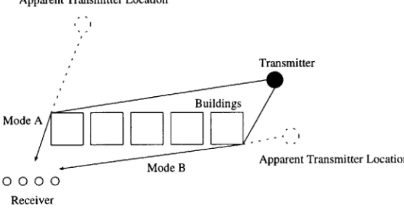
the actual transmitter. Figure 1 illustrates a situation where the elimination of
modes is useful.
Figure 1 shows two modes incident upon the receiver. Mode A gives an
Apparent Transmitter Location
Transmitter
-' Buildings
Mode A
-Apparent Transmitter Location 0000
Receiver
Figure 1: An urban phone call.
gives an apparent transmitter location which is much closer to the true location.
Since mode B gives a much better approximation of the transmitter location,
we want some criteria for eliminating mode A while keeping mode B.
Several criteria can be used to judge modes for possible elimination. These
include mode power, direction of arrival, and relative time of arrival. In general,
modes with higher power will provide better estimates of the true transmitter
location, since higher powered signals have usually bounced around and changed
directions fewer times. The direction of arrival is a good elimination criterion
when there are many modes. If most are arriving from the same general
direc-tion, but one mode is significantly off, then that mode can likely be eliminated.
The time of arrival is another way to judge what path a signal has taken on
its way to the receiver. Modes which arrive earliest have usually taken the
most direct path to the receiver and thus provide the best estimates of receiver
location.
ap-Transmitter
Wavefronts
0000
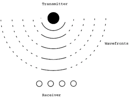
ReceiverFigure 2: Decreasing curvature of a wavefront with distance.
proach looks at a wavefront's curvature as an additional source of information.
A wavefront's curvature might be important, because curvature changes as a function of distance, just as the curvature of a circle changes as a function of
its radius (figure 2).
Let us refer back to the problem depicted in figure 1. Mode A originates from
diffraction about a nearby building. Mode B originates from diffraction about a
far-away building. As we will see in section 2.4, when an electro-magnetic wave
diffracts around an edge, the edge appears as if it were a new (two dimensional)
point source. Thus mode A exhibits relatively high curvature, while mode B
exhibits relatively low curvature. Knowing these curvatures, it is possible to
eliminate mode A because of its having originated from a local scatterer. A
scatterer.
This project will analyze the utility of estimating a wavefront's curvature to
eliminate misleading modes. This project does not, however, attempt to "solve"
the geolocation problem in the fullest sense. Geolocation in a complicated urban
environment is very difficult, and any technique that can help in even a small
number of scenarios is important. Distance estimation using wavefront
curva-ture is also a difficult problem. This is particularly true in view of the inevitable
phase errors, or calibration residuals, which occur in a physical antenna array.
However, three factors particular to this project serve to mitigate estimation
difficulties. First, the distances in question are relatively small, on the order of
several hundred meters. Second, the antenna array aperture is very large, on
the order of tens of meters. Finally, estimates need not be accurate, only good
enough to judge one scatterer farther than another.
2
Background
2.1
Direction Finding Algorithms
Here we give a brief sketch of the derivations of two important direction finding
algorithms. See Krim [12] for further details.
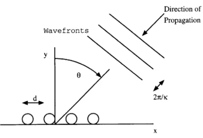
For a uniform linear array, let the antenna elements lie along the x axis with
an element spacing of d, and assume an incident sinusoidal plane wave at angle
O to the y axis with frequency w and wavenumber k (figure 3).
Direction of Propagation Wavefronts y 0 2n/K x Antenna Elements
Figure 3: Plane wave incident on an antenna array.
a different phase part of the wave hits the second element. The phase difference
is found by multiplying the wavenumber by the amount of extra distance the
wave has to travel to get to the second element, given by -kd sin(0). The minus
sign indicates the assumption that the first antenna element is farthest from
the wave source. A steering vector, V(O), is then defined for the antenna array,
where
?
(0) = g(0) 1 e-jkdsin(O) e-jk2dsin(e) ... e-jkndsin(O)and g(O) is an an antenna element's gain in the direction 0. V(6) gives the
si-multaneous responses of each antenna element to such a plane wave. In defining
?(0),
we have designated the plane wave to be at zero phase at the first antennacase 7(6) is multiplied by the phaser est, yielding
T
?(0)
= ejg(0)[
1 e-ikdsin(0) e-ik2dsin(o) ... e-jknsin(O)= g(O)
[
ej e(-kdsin()) O ej(-k2dsin(9)) ... ej( -kndsin(e)) IThe notation of the steering vector may be generalized to a nonuniform or
even non-linear array. If we denote the 3-D spatial location of antenna element
m by im, and define the vector k such that its magnitude is the wave number
and its direction is the direction of wave propagation, then we can write
V(6) = g(0) eJI
zi
eis2 - ... e- ISo long as an incoming signal, s(t), is of narrow bandwidth, and k does
not change much amongst the signal's frequency components, the array output
vector in the zero-noise limit is given by
F(t) = f()s(t)
With beamforming techniques, a weighting is applied to the array output
vector such that the antenna element responses for a signal arriving from a
particular direction will be added in phase. Thus, if a signal happens to be
arriving from a direction 0, then a weighting designed to maximize power from
00 will give a very large output. By varying the weighting to maximize power from different directions, it is possible to search over all directions looking for
incoming signals. Peaks in a plot of power versus direction will indicate probable
signal sources. The weighting will vary based on different optimization criteria.
when multiple modes are widely separated in direction [12]. For this project,
where we assume only a single mode, beamforming techniques are adequate.
However, when there are closely spaced multiple modes, other direction finding
algorithms, such as MUSIC, can be used to resolve the modes [2].
When multiple signals are present, the steering vector, V(O), becomes a
matrix, V, where each column of V is a steering vector corresponding to a
distinct direction, 0. If additive noise is taken into account, then the array response vector becomes,
5(t) = Vs(t) + i(t)
If the noise is spatially white, then n-(t) has covariance u21. If the signal source has covariance P, then the covariance of the array response to signal plus noise
is given by,
R = VPVH + a21
where the signal and noise are assumed to be uncorrelated. With M signal
sources, P is MxM. It is also assumed that P is full rank (different signals are
incoherent). It is further assumed that steering vectors for disparate directions,
0, are linearly independent, and thus V is of rank M, and therefore VPVH is of
rank M. With this assumption together with VPVH being a covariance matrix,
it follows that VPVH is positive semidefinite, with M positive eigenvalues and
L-M zero eigenvalues, L being the number of rows in V (the number of antenna
elements). Now for any eigenvalue, A, of R, there will exist an eigenvalue,
A - a2 for VPVH, implying that A - a2 > 0, and thus A > o2. Where a
A is exactly equal to o2. The null-space of VPVH can then be constructed from the L-M eigenvectors of R corresponding to the L-M smallest eigenvalues,
each of which will be equal to o2. Once the null-space is constructed, the
steering vectors in V corresponding to M unknown directions may be found by
virtue of their orthogonality to the the null-space of V. MUSIC plots a function
of 0 which contains the magnitude of the null-space component of a possible
steering vector, V(0), in the denominator. A steering vector with no null-space
component will make the denominator go to zero and cause a large peak in the
plot, corresponding to a direction of arrival.
Quite a number of other direction finding algorithms exist. Many are
de-signed to overcome certain difficulties, such as closely spaced or coherent signals.
Others make efficient use of particular array geometries [12]. A common end
result involves the plot of some function versus direction, where peaks in the
function indicate signal directions of arrival, or modes. For the purposes of this
project, it is then a matter of winnowing down the number of modes.
2.2
Generalized Beamformers
The appearance of a non-planar wavefront at an antenna array is treated briefly
by Cadzow [7]. Without the planar assumption, the steering vector takes on a more complicated form. In particular, assume a point source is located at p- in
three space. The antenna elements are at points Xm where m is the element
number. Then the distance, dmi, from the source to the mth element is given by
If 5 corresponds to direction 0, and average distance r, then the steering vector
may be written as
V(r, 0) = g(r, 0) e-jkd1 e-ikd2 e-ikda . e-jkan
Putting the first antenna element at zero phase gives
V
(r, 0) = g(r, 0) 11 eijk(d1 -d2) ejk(d1-d3) .. eijk(d1-d.)Baggeroer [1] talks about a generalization of beamforming techniques to
looking for point acoustic sources. The technique involves anticipating the fields
from a source at a particular location, and applying a weighting to the antenna
elements which maximizes the power received from that location. In this way, all
locations may be searched over to see which produces maximum power output.
This is just beamforming for both r and 0. Bucker [6] goes into even more
detail.
We may further generalize beamformers to maximize the array response for
any kind of wavefront. In essence, we create a spatial matched filter which
matches the spatial structure of any anticipated wavefront, be it point source or
otherwise. Thus, if we expect a wavefront which results from the diffraction of
a plane wave about a half-plane, then we can phase the antenna array so that
each element's phase is the conjugate of the phase from the incoming wavefront.
We prefer not to have to tailor such a matched filter to every specific
wave-front, however. We would rather pretend that every incoming wavefront results
from a point source. Why is this? First of all, using a point source model is
from the source to each antenna element, a calculation which is easy knowing
the x and y coordinates of source and element locations. In contrast, using
the true field as a model for forming a steering vector at each search location
entails calculating the electric field coming from a hypothetical source at each
location. As is apparent from examining the analytic solution (see equation 1),
this calculation is considerably more complicated than simply finding a distance.
Furthermore, if one does not know the true nature of a source, one has to use a
number of models simultaneously.
Secondly, we postulate that a point source model is a very good
approxima-tion for wavefronts arising from other types of sources. We have in mind the
wavefront resulting when a plane monochromatic wave diffracts about the edge
of a half-plane. In fact, according to the widely used geometric theory of
diffrac-tion, the edge of a half-plane acts exactly like a two-dimensional point source
with regards to phase. Whether or not a point source model proves sufficient is
the major part of our investigation.
2.3 Electro-magnetics
This project seeks to estimate the distance from a receiving antenna array to
the source of a mode. A mode might be line of sight, or the result of reflection,
refraction, scattering, or diffraction. To get a distance estimate from the antenna
to, say, a diffracting object, it is necessary to see how the diffracting object will
distort, and thereby add curvature to an incoming wavefront.
electro-magnetic wave has been of interest in the literature for quite some time
[4]. In general, there is no closed form solution for a resulting field. For this
general case, one might consult Bertoni [3], which deals with many ways of
combining numerical and analytical methods in modeling electro-magnetic wave
propagation in complicated environments. It is more desirable, however, to
work with objects for which a closed form solution is known, since distance
estimates may be very sensitive to approximations or small numerical errors in
field calculations. Bowman [4] describes a number of objects for which fields
have been analyzed. King [10] also addresses a number of simple objects (though
not the half-plane), but provides a somewhat more tractable analysis.
The half-plane was one of the first objects for which an analytic solution
was developed [4]. Furthermore there exists extensive literature on the subject.
This is convenient in that an infinite half-plane may be used as a simple model
for the side of a tall building in an urban environment.
The signal incident upon the side of the building is modeled as a
monochro-matic, z-polarized, electro-magnetic plane wave. The z direction is taken to be
up, and is parallel to the edge of the half-plane (figure 4). If the point source
of the incident signal is reasonably distant, then a plane wave is a very good
approximation to the otherwise spherical wave.
One representation of the resulting electric field is given in equation 1.
-e 1
E = 4 {e-ikCos(0-00)F[- 2kpcos - - #)]
1
-e-ikpcos(0+0)F[- 2kpcos I(+$0)]} (1)
x direction of propagation
bright side of half-plane shadow region of half-plane
Figure 4: The diffraction of a plane wave about a half-plane.
The function, F(r) is the Fresnel integral, defined as
F(r) =
j
ep
2dpThe Fresnel integral can be written as
F(r) = {[ - C( r)] + i[- S( 2)]}
where C(u) and S(u) are given by
C(u) = Cos( 1et 2
)dt
S(u) = I sin( 2rt 2)dt
The representation of F in terms of C and S is useful because C and S are
native to the Mathematica programming environment.
Of particular importance to this project is the phase of the electric field. Phase may be calculated simply by taking the arctangent of the imaginary part
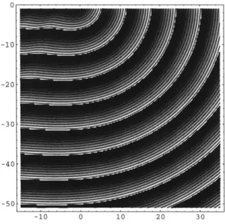
over the real part of the field function, Ez. A sample contour phase plot is shown in figure 5. Similar plots may be found in Braunbek [5].
0 -10 -20 -30--40 -50 -10 0 10 20 30
Figure 5: The diffraction of a plane wave about a half-plane, based on the
2.4
Geometrical Optics and the Geometric Theory of
Diffraction
Geometrical optics is the simplest and most widely used theory of
electro-magnetic wave propagation [9]. The basic premise is that light travels in straight
"rays" from a source to a destination. The electric field at a point on a ray is
determined by the distance to the source and by the geometry of the source. So
if r is the distance to the source, and k is the wavenumber, then the phase of
the electric field is given by
4o
- kr, where0
is the phase at the source. If the source is a line source, then the electric field amplitude goes as E0/rA, while ifthe source is a point, then the electric field goes as Eo/r. For more complicated
sources, fields may be found as sums or integrals of fields on rays emanating
from multiple or differential source elements.
Geometrical optics also includes a provision for reflected rays. This is the
familiar law of reflection, where the angle of an incident ray equals the angle of
its reflected ray.
Traditional geometric optics is easy to use and provides good approximations
in many cases. However, it does not account for the presence of electro-magnetic
energy in shadow regions, where a source is completely obscured by an obstacle.
Figures 6 and 7 give plots of electric field amplitudes for plane waves incident
upon a half-plane. Note the difference between the the geometrical optics
solu-tion, and the exact solution. Plots similar to figure 6 are given in a number of
references, such as Kong [11] and Braunbek [5].
geomet-field magnitude -i'0 8 -2 0.8 0.8 0.4 0.2L 20 x
Figure 6: Field magnitudes according to the analytic solution. These
magni-tudes were plotted over the contour, y = -1000A. Negative values of x
corre-spond to the bright region of the half-plane, while positive values of x correcorre-spond
to the shadow region.
field magnitude 1i 0.8 0.6 0.4 0.2 -100 -80 -60 -40 -20
Figure 7: Field magnitudes according to geometrical optics, before diffraction. x
, ,2,,
rical optics to include diffracted rays in addition to incident and reflected rays.
Diffracted rays result when an incident ray hits a sharp edge or a point. Since
points and edges are non-differentiable surfaces, it had not been clear at what
angle rays should depart when happening upon these. Keller postulates that
rays may emanate from a point in any direction, and from an edge in any
di-rection constrained to lie on a cone. He then gives diffraction coefficients which
depend on the angle of incidence and the angle of diffraction. These diffraction
coefficients are found by matching the fields given by geometrical optics to the
fields given by exact solutions.
In spite of Keller's improvement, geometrical optics still provides only an
approximation of true electric fields. For one thing, we note that diffracted rays
in the shadow region of an obstacle bounded by an edge all seem to originate
from that edge. The phase fronts of the wave in the shadow region form a
perfectly cylindrical wave (when the incident wave is planar). But while this
is very close to being true, and provides a justification later on for treating a
half-plane's edge as a line source, it is not really the case. Thus, in this paper,
we make use of the exact solutions when simulating the diffraction of a plane
wave about a half-plane.
2.5
The Sparse Array
Dr. Dan Bliss, of the MIT Lincoln Laboratories, devised an antenna array for
some cellular experiments that Group 44 at the lab is doing. This is a sixteen
fre-quencies (A = .15m). The antenna was designed using a genetic algorithm with
the intent of minimizing side lobes. Since the the aperture is wide compared to
the number of antenna elements, the array is "sparse." I use this antenna in my
own simulations, and hence refer to it as the "sparse array."
2.6
Array Errors
The main test of an array which uses wavefront curvature as a distance estimate
is its performance under less than ideal conditions. The curvature in a wavefront
is generally very gradual, and any small distortions can completely scramble the
inherent information.
There are many sources of error that may effect an antenna array. These
include tolerance limits on array hardware components, feed-line length errors,
element misplacement, quantization error in discrete phase shifters, bit failures,
amplifier failures, and so on. Usually the designer tries to eliminate all errors
which are correlated from element to element, so that what remains are residual,
uncorrelated phase and amplitude errors [13].
In addition to the residual error introduced by the array components, there
is also thermal noise present with the signal. However, in our application we
will be able to integrate the received signal over long periods of time, effectively
eliminating any thermal noise problems.
Forsythe [8] gives a model for residual array errors as "a vector of
inde-pendent, identically distributed, complex circular Gaussian random variables"
residual errors through the signal power, P. If the noise power introduced by
residuals is normalized to unity, then P oc 1 , where c is the variance of the
components of the error vector. The variance e is derived over an ensemble
of possible antenna arrays since, unlike thermal noise, residual errors remain
constant for a given antenna array.
With the assumption that residual component errors are the dominant source
of error, and provide us with Gaussian noise uncorrelated from element to
ele-ment, and uncorrelated with the signal itself, we proceed with a derivation of
bounds on the range estimator.
3
Cramer-Rao Bounds
3.1 Definitions
For a given mode, we wish to estimate the range and angle of its source. We
do not know the signal power a priori, so we are also left to estimate power as
a nuisance parameter. We define a parameter vector,
D5 [p r6]T
which is the vector of parameters we are trying to estimate. Our estimate of D
is defined as
D = [p r 05]
We do not observe the parameters in D directly. Rather, we observe some
case, the observation vector is the array output vector which we call XF(r, 6)
below. From W, we determine D.
The Cramer-Rao bound inequality gives us lower bounds on the variances
of the estimators in D provided they are unbiased. These bounds are derived
from the inequality,
C > Pcr
where C = Y9H is the covariance of the observation vector and
_1 62In p(WgID)
[Pc. ]g = -E
{
-.defines the Cramer-Rao bound matrix, whose inverse, P-1 is called the Fisher
information matrix [19]. Smith [19] also treats the case where estimators are
biased. Cramer-Rao bounds tell us how well we can hope to do with our
geolo-cation scheme.
3.2 Derivations
Let the antenna lie along the x axis with elements having the x coordinates
X1, X2, ... X. The variable r will denote the distance of a source from the origin,
and the variable 0 will denote its angle measured clockwise from the positive y
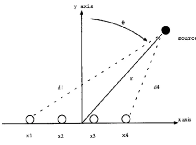
axis. Figure 8 illustrates this.
The distance from a point source located at (r, 0) to an antenna element
located at (Xm, 0), may calculated with a little trigonometry, and comes out
to be dm =
fr
2 - 2r Xm sin(0) + x2. The array response to a point source is then (r,60) = [ei k dl e-jk d2 ... e-jkan], where here and henceforth wey axis 0 - source di d4 x axis x1 x2 x3 x4
Figure 8: The physical meaning of the symbols used in the bound derivation.
assume that antenna elements are isotropic (g(r, 0) = 1). If we assume that the
incoming signal has power P which does not vary significantly over the span of
the array, then the array response is v/ishZ. Finally, we include additive noise.
Thus, i(r, 0) =
\/iz+
n-. We now seek to find the covariance matrix, C, for i.In what follows, angular brackets denote time averaging.
C = (zzH)
((pZH + )(-/ 5l+) H+ HH
+
Now when we constrain n' to be zero-mean spatially white Gaussian noise, we
find that the second and third terms go to zero. This is because F and n- are
uncorrelated and zero-mean. If we also normalize the signal and noise powers
such that the noise power is unity, then the fourth term is just the identity
matrix. Thus
and P is measured in units of noise power. Plugging in the elements of -, we get 1 e-j k(d1-d2) . - k(d1-d ) ej k(d1-d2) .. e-i k(d2-d.) C=P +I e jk(di-d,) e k (d2 -dn,) .. . 1
The Slepian-Bangs formula for a Cramer-Rao Bound matrix where the
ob-served data has Gaussian distribution is given in Appendix B of Moses [17].
The element-wise formula is
1
= [ tr[C-1C'C-lC + [ TC- ] 2
c-C~ic[2]
+[iZ
T',73
where C is the covariance matrix of the observation vector Y, /I is the mean of
, C is the derivative of C with respect to the ith element of -, and
#
is the derivative of f with respect to ith element of Y.The derivative of C with respect to P is easily given by
1 e-i k(d1-d2) -jk(d1-d.)
j k(di-d 2) . e-j k(d2-dn)
' == (C - I)
ej k(d, -d.) ejk 02 -d.) .. . 1
In calculating the derivatives of C with respect to r and 0, we look at a typical
element of C, ejk(dp-d,).
d (ej kp-dq)) = jkei k(dp-d)
d(dp - dq)
dr3
= j k ej(dp-d ) r - xP sin(O) r - x sin(O) 2 - 2r x, sin()
+t
x2 2 - 2r xq sin(O) + xJ
p qP -jkik(dp-de) r-XP sin(0) d, r- xqsin(O) dqIn a similar fashion, we find that
d (ej k(dp-dq)) d6 dj k(d)-dq) d _ .k ej k(d - dq) r x P cos(0) dP r Xq cos(O) dq
Had we instead looked at e-s k(dpdq) we would have obtained the same
results, except with negative signs out front and in the exponent. We have
then,
0
e k(di-d.) r'-xi "in(O) - r-x si"(O)
0
.. -e-i k(di-d.) rxsnO
0
-e-i k(di-d.) ( rxas(') + rXn COS())
ejk (di -d) -r Xicos(6) r Xcos(O) 0
To find the inverse of C, we use
C- 1 = - I
nP+ 1
which only works because C is the sum of the identity matrix and a rank-one
matrix [15]. We verify by taking the product CC-1.
CC- = C
I
-C -1 ) nP +1 C'. = jk P and C' =jkP r - x, sin (0)d,
= C(I- n+1 I) CPiiH = C nP+1 C nP+ 1 C p2FHFH + pH p2ggH ggH+ pggH = C-p2- - 2gFH + pggyH nP+ 1 pFFH (nP p 1) = C nP+1 PiH+IPpnP+1 =PiiH + I _ pgj*H = I
Now, with our zero-mean noise, we may discard the second term in the Slepian-Bangs formula, and we have
[ = tr[C 1CC' C'p] [Pc1]1 2 = Ifr[C~1C'pC- 1C'] [P-1]13 = 1tr[C-IC' C- C'] [P ]2 1 2= 0tr[C-CC'C'p] [P~']2 2 =
~tr[C~C1C'ClC,]
[Pc~] 2 3 = 1tr[C1C'C-1C] [P-.] 3 1 = C'C1C'p]rr[C [P-.I
rCI[P; 1]3 3 = fr[C- C'C-C'G]
Of these, [P-] 11, may be expressed compactly.
[P-] 1 1 r C ~ 2 Str[(C-1 C'p) 2] 2 t
1
r I- C- 1 (C - I)) 21 P H P2 = tr I -PiH p 2y)2] 2p2 nP+1 1 tr nP~yH 2 =~p 2P-H 2P1H 12(nP )2 H 2p2r nP + 1~y
nP +rn~y pjI 1 1 (piH )2' tr nP 1 2(nP + 1)2tr [(i*;H ) 2(nP + 1)2 n2 2(nP + 1)2Unfortunately, there appears to be no compact way of expressing the other
elements of P-1 in terms of n, r, 0, d's, and x's. We thus turn to a typical
example of Pcr. Our array is the sparse array and our point source is located
at (r, 0) = (3333A, -L). Also let P = 1000 which puts the signal power at 30dB
over the residual power. Then
A) Ap, Ap 1.000 X 10⁶ 3.745 x 10⁻⁸ -2.060 x 10 Per = A~p Af A,g = 1.056 x 10⁻⁸ 560.2 -1.386 x 10
Agg Aj, Aj 1.004 x 10⁻¹³ -1.386 x 10~5 7.236 x
10--14
-5
This matrix was calculated numerically using Mathematica. To compare A,;
with Aj, we convert Ag from units of radians squared to wavelengths squared
using the factor 33332. We get Aj(A2) = 8.038 x 10³. Note that the variance on
the range estimator is very high compared to that on the angle estimator. This
is what we would expect, since there is very little phase delay from element to
element due to a wavefront's curvature, while there is much more phase delay
from element to element due to a wave's direction of propagation. We also
expect that this matrix would be symmetric. In particular, Ap, = Afp and Apj = Ajp should hold. However, these covariances are apparently so negligible that significant numerical errors creep in. We are not particularly worried about
these entries in P, but mainly about A,.
Let us look at some plots of Cramer-Rao bounds. There are three parameters
to consider. These are range, angle, and signal power, relative to a unit noise
power. Figures 9 and 10 show bounds on the standard deviation of a range
estimator for different source ranges, angles, and signal powers. The sparse
array is used in calculating these. Let us see that these make sense. First, the
variance on the range estimator, Af, increases as the range of the true source
increases. This is quite logical, since curvature is very tiny for sources at a
distance and does not change much as distance increases even more. Secondly,
A1 decreases with increased signal power relative to a constant noise power. Of
course smaller residual corresponds to a better estimate. Finally, A,; increases
as the source angle approaches 1 or - , and in fact reaches oo at these angles. This is because, as 0 approaches 1, the array spans a smaller and smaller portion
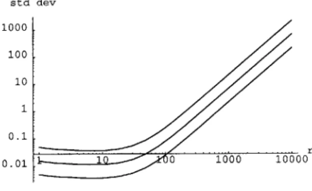
std dev 1000 100 10 1 0.1 r 0.01 1 0 1000 10000
Figure 9: Bounds on the standard deviation of range estimators for SNR of 10,
20, and 30dB, plotted at 0 = 0. The top curve is for 10dB. The bottom is for
30dB. Axes units are in A.
of the source's radiating arc, until, at , the array cannot see any curvature at
all since the source lies along the array axis.
Let us also examine what happens when we reduce the array aperture. We
use a sixteen element array with a uniform element spacing of . Figure 11
shows a comparison between the bounds for the sparse array and the bounds
for the small aperture array.
4
Methods
Many of the findings in this project stem from the performance of numerical
simulations. This section indicates the software with which the simulations are
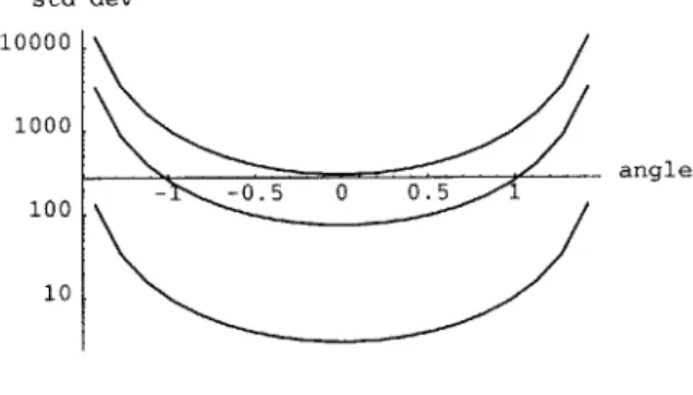
std dev 10000 1000 100 10 L - -0.5 0 0.5 1 angle
Figure 10: Bounds on the standard deviation of a range estimator plotted at
ranges of 667A, 3333A, and 6667A (100m, 500m, and 1000m). The top curve is for 6667A. The bottom curve is for 667A. SNR is 20dB. Horizontal axis units
are radians. Vertical axis units are A.
std dev
1000
10
0.1
1 10 100 1000 10000
Figure 11: Bounds on the standard deviation of a range estimator plotted at
0 = 0. The top curve is the bound for a small aperture array, while the bottom is the curve for the sparse array. Axes units are A.
4.1
Software
The simulations performed in this project are done in Mathematica, Version 3.0
running on a Sun. Mathematica is used for its strong numerical and graphing
capabilities. Of special attraction is its built in Fresnel integral function, which
is widely used in this project. The down sides of Mathematica are that its matrix
manipulation and scripting capabilities are not as smooth as those of Matlab.
Also it crashes quite frequently. Alternative software choices are described in
Mirotznik [16].
4.2 A Typical Simulation
A typical simulation involves designating a position for the source and then allowing the array to search over a given area to try to locate the source. By
"gsource'' , we refer to the edge of a half plane with an incident plane wave.
The source lies somewhere in the upper half of the x, y plane, while the array
elements lie along the x axis. The number of elements and their positions on
the x axis may vary depending on what antenna is used in the simulation.
A simulation first determines the true electric field, E, at each antenna array element. It uses equation 1, the analytic solution of a plane wave's diffraction
about a half plane, to determine the electric fields. The phase is then
#
=tan-
E), with adjustments made for the second and third quadrants. Once the phases of the true field are known at each antenna element, they areformed into an array response vector, F = [e-i OE1 e-' "E2 ... en OE.]T. The
desirable and is certainly a topic for further research.
Next the antenna array searches over a given region for the source. For
each possible source location (x, y) that the array looks at, the array forms
a steering vector. The steering vector is the array response that would occur
from a point source at (x, y). Thus, if the distance from (x, y) to element m is
dm, and the wave number is k, then the steering vector is given by V(r,0) =
[e-J k di e-jk d2 ... e-j k d]T . Note that the steering vector is just the weighting
applied to the array response in order to produce a beamforming statistic. The
statistic, S, is then formed where S =|I(r, 6)H 2. The S statistic is plotted as
a function of search locations. When the search location corresponds to the true
source location, we have V(r, 0) ~
i, assuming the antenna is in the shadow
region. Then S ~_I|4
which is the maximum value S could possibly attain. S probably never quite attains its maximum value, however, because the weightingis designed for a point source wavefront rather than a wavefront resulting from
diffraction about a half-plane. Still, it comes very close.
Another way to think of the search the array performs, is simply as a sweep
of its antenna pattern over a two-dimensional space. In simple direction finding,
the antenna pattern is simply a function of angle, and the pattern may be swept
across all angles [-!-, f]. Plane waves originating from some angle produce a
strong response when the mainbeam of the antenna is pointing in that direction.
In our case, the antenna pattern is a function of both range and angle. So the
search must span over two dimensions in order to find the coordinate, (ro,
0),
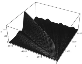
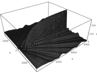
which produces the strongest response, or S statistic.We now show a few examples of S statistic plots. Figures 12, 13, 14, and
15 are plots where the source has been placed somewhere in the x, y plane and corresponding S statistics have been plotted. These plots may be interpreted by
first imagining the antenna array at the origin. Then for each (x, y) location the
antenna examines, it plots the S statistic. Points in the x, y domain for which
S is high show what locations give the antenna array a strong response. The
(x, y) location which gives the highest peak is assumed to be the true source location.
By visually inspecting the plots, it is very easy to tell what angle the source is at relative to the antenna array. The sharp radial ridge gives this away.
However, along that ridge, it is very hard to tell where the highest point is.
This is the problem of finding the range. One benefit of this ridge structure we
will make use of, is that we can significantly reduce the amount of searching
needed to find the global peak. Instead of looking everywhere in the x, y plane,
we need only find some point on the ridge and then walk along the ridge until
we find the global maximum.
Now let us take a closer look at the predictions the plots make. Since we
know in advance where the true source location is, we are in a position to judge
how accurately the statistic predicts it. The first three plots look about right.
When the true source location is at an angle of - I, or -
I,
the large ridge makes the same angle with the positive y axis. However, in the fourth plot,the source is at an angle of 1, yet the ridge indicates that the source makes
6000 4000 200 S 100 - 2000 0 0 -400-2000 0
Figure 12: S statistic plot for a half-plane source location at (r,0) =
(667A, - ) = (100m, -i). Axes units are in A.
the array is in the shadow of the half-plane, and it homes in on the edge of the
half-plane, since the edge looks a lot like a point source in the shadow region. In
the fourth plot, the array is in the bright side of the half-plane. So it homes in
on the distant point source which is producing the incident plane waves. Since
the incident plane waves propagate in the direction of the negative y axis, the
ridge in the fourth plot is along the y axis. This is, in fact, the result we want.
The distant point source gives a better estimate of the transmitter location than
S
6000
Figure 13: S statistic plot for a half-plane source location at (r, 9)
(667A, -1) = (100m, -1). Axes units are in A.
6000 4000 y 200 100 2000 0il. -6000 -400 -2000 0
Figure 14: S statistic plot for a half-plane source location at (r, 0)
Figure 15: S statistic plot for a half-plane source location at (r, 0) = (667A,
})
= (100m, 1). Axes units are in A.Apparent transmitter
-. direction for
', rray 2
True transmitter location, apparent transmitter location for array 1
oo 'o 00'00
Array 1 Array 2
Figure 16: Antenna arrays in the bright and shadow regions of a half-plane
trying to locate a transmitter.
5
Simulation Experiments
In this section we will discuss several experiments. These are not field
experi-ments, but simulations performed using the Mathematica programming
environ-ment. Code is given in the appendix. All results are deferred to the "Results"
section.
5.1
Obtaining a Precise Angle Estimate
The S statistic is a continuous function of two variables for some given
antenna-source configuration. Using computers to calculate the S statistic, we must face
the issue of sampling.
In our first experiment, we test how finely it is necessary to search in the
angle dimension in order to obtain a precise angle estimate. We say that an
angle estimate is precise when finer and finer searches fail to give a significantly
different angle estimate. Our searches are performed over the upper half plane
from 0 = -2 to 0 = ', and from r = A to r = 66667A = 10000m. The r dimension is sampled logarithmically. In other words, more range samples are
taken near the array than farther away. The reason we restrict our search to
10km is that by this range, there is virtually no discernible information in a
wavefront's curvature. It looks just like a plane wave.
The antenna array we use is the sparse array. We place a source, the
half-plane, at a fixed range of 100 meters, equivalent to 666.67A at A = 15cm.
We vary the angle of the source in the array's field of view, so that the source
* Source Locations
a 500 100e
1000m
100m
Antenna Array
Figure 17: Source locations for testing the beamformer. Note that the black
dots represent the edges of a half-plane, not point sources.
the array does several searches to see if it can find the source. These searches are
performed with 200, 400, 800, 1200, and 1600 samples in the angle dimension.
We then repeat the same procedure, but with the source range fixed at 500
meters, and then with the source at 1000 meters. Figure 17 shows the locations
the source is tested at.
5.2
Separating Range and Angle Searches
We wish to cut down on computation by finding an angle estimate before finding
a range estimate, rather than finding the two simultaneously. This seems feasible
due to the fact that range and angle estimates are highly uncorrelated. The
computational savings comes from doing two approximately one dimensional
searches as opposed to one two-dimensional search.
In this experiment, we use the results of our prior experiment (see section
6.1), and perform a search which has 800 samples in the angle dimension. There are initially only 10 samples in the range dimension. We obtain an angle estimate
from this search. We use this angle estimate to narrow our search to a small
arc centered on that angle estimate. Within this small arc, we perform a much
finer search in the range dimension, with 200 mesh points instead of 10. The
number of angle mesh points remains proportional to arc length.
Specifically, our second experiment determines how small our estimate-centered
arc may be while still yielding precise range estimates. The arcs tested are 1,
1,
n,
and - radians. Once again, the true source is placed at ten different201 40' 80
angles for each of three different ranges.
5.3
Accuracy of Range and Angle Estimators
Our concern up until now has been making sure that we are searching finely
enough to extract all available information from the source's true signal. In other
words, if there are maxima in the continuous S statistic curve, we are going to
find them. We have not yet determined, however, whether such maxima truly
represent the source's location. There is a reasonable chance that these maxima
may not be accurate, since our true source is a half-plane, while we are searching
for a point source.
Therefore, this experiment will test the accuracy of our angle and range
estimators for a number of different source locations. We will again test the
three ranges of 100, 500, and 1000 meters. However, we will look at 30 arc
5.4
Filled Array
The results of the accuracy experiments, given in figures 24 and 25 in section 6,
indicate errors in range and angle estimates for nearby source angles between
- ' and 0. With this experiment, we wish to examine the cause of these errors. The likely cause is that the array we have been using is a sparse array. Sparse
arrays are known to possess high side lobes which can be a cause of ambiguity.
We thus replace our sparse array with a filled array of approximately the same
aperture. Our filled array has 201 elements spaced ' apart. We examine 30
source angles at a range of 100 meters.
5.5
Small Aperture Array
The erroneous results we achieved at 100 meters with our sparse array might
also be due to the wide array aperture. We note that in the region directly
behind the edge of the half-plane (close to the negative y axis), the wavefront is
in transition, morphing from a plane wave in the bright region into a cylindrical
wave in the shadow region. Either of these two types of waves may be attributed
to a point source, at infinity or nearby, respectively. However, it seems likely
that when half of the array is in the plane wave region, and half of the array
is in the cylindrical wave region, the array will not be able to get a very good
fit to a point source anywhere. It is under these circumstances that ambiguities
might occur.
Therefore, we make the array aperture much smaller, so that it is much less
element array with an element spacing of A. Again we make range and angle
estimates for a true source at 30 different angles for ranges of 100m, 500m, and
1000m.
6
Results
This section presents the results of our simulation experiments.
6.1
Obtaining a Precise Angle Estimate
Figures 18, 19, and 20 show the three plots of angle estimate versus true source
angle and search mesh, one plot for each range.
We see from the plots for the three different ranges, that our angle estimate
as a function of true source angle only becomes precise when a mesh with 800
samples in the angle dimension is used. We conclude that 800 samples is a safe
minimum number of samples to use in the angle dimension for estimating the
true source angle.
We can check this result with a theoretical calculation. An antenna's angular
pattern is known to have a Fourier transform relationship to its aperture. Thus,
the angular beamwidth of a linear array is approximately equal to :, where L is
the length of the aperture [20]. For the sparse array, this gives a beamwidth of
1 radians. Dividing this into the 7r radians over which we perform our search, and sampling three times per beamwidth, we get approximately 900 required
0.5 0 angle estimate -0.5 -1 0 angle 1
Figure 18: Angle estimate as a function of the fineness of a search in the angle
dimension. Range is fixed at 667A = 100m. The vertical and horizontal axes'
0 angle -0. 5 estimate -1 0 angle 1
Figure 19: Angle estimate as a function of the fineness of a search in the angle
dimension. Range is fixed at 3333A = 500m. The vertical and horizontal axes'
angle estimate
0
-1 0
angle
Figure 20: Angle estimate as a function of the fineness of a search in the angle
dimension. Range is fixed at 6667A = 1000m. The vertical and horizontal axes'
We have not yet said anything about how accurate our angle estimate is,
only that it is precise when we take 800 samples in the angle dimension.
6.2
Separating Range and Angle Estimates
Plots of range estimates versus true source angle and arc length are shown in
figures 21, 22, and 23. Our results suggest that precise range estimates exist
only for a minimum arc length of -. For the two smaller arc lengths, there is
a sharp peak in the range estimate at a true source location of (100m,
j).
6.3
Accuracy of Range and Angle Estimators
Figures 24, 25, 26, 27, 28, and 29 show range and angle estimates as a function
of true source angle for ranges of 100, 500, and 1000 meters.
The results of this experiment suggest that range and angle estimates are
accurate for source angles less than 0. The exception is when the source range
is only 100 meters, in which case range and angle estimates are only accurate
below source angles of - 1. When we account for the fact that the array is
in the bright side of the half-plane for source angles greater than 0, we can
interpret our estimates as estimates of the source of the incident plane waves
rather than as estimates of the edge of the half-plane. With this interpretation,
our estimates become accurate for all angles greater than 0. Our only remaining
source of significant error is when the half-plane is nearby and at angles ranging