HAL Id: hal-00318330
https://hal.archives-ouvertes.fr/hal-00318330
Submitted on 29 Jun 2007
HAL is a multi-disciplinary open access
archive for the deposit and dissemination of
sci-entific research documents, whether they are
pub-lished or not. The documents may come from
teaching and research institutions in France or
abroad, or from public or private research centers.
L’archive ouverte pluridisciplinaire HAL, est
destinée au dépôt et à la diffusion de documents
scientifiques de niveau recherche, publiés ou non,
émanant des établissements d’enseignement et de
recherche français ou étrangers, des laboratoires
publics ou privés.
their disparities in remote sensing of the ocean colour
P. Shanmugam, Y. H. Ahn
To cite this version:
P. Shanmugam, Y. H. Ahn. Reference solar irradiance spectra and consequences of their disparities
in remote sensing of the ocean colour. Annales Geophysicae, European Geosciences Union, 2007, 25
(6), pp.1235-1252. �hal-00318330�
www.ann-geophys.net/25/1235/2007/ © European Geosciences Union 2007
Annales
Geophysicae
Reference solar irradiance spectra and consequences of their
disparities in remote sensing of the ocean colour
P. Shanmugam and Y. H. Ahn
Ocean Satellite Research Group, Korea Ocean Research and Development Institute, Ansan P.O. Box 29, Seoul 425-600, Korea Received: 5 February 2007 – Revised: 26 March 2007 – Accepted: 31 May 2007 – Published: 29 June 2007
Abstract. Satellite ocean colour missions require a stan-dard extraterrestrial solar irradiance spectrum in the visible and near-infrared (NIR) for use in the process of radiomet-ric calibration, atmospheradiomet-ric correction and normalization of water-leaving radiances from in-situ measurements. There are numerous solar irradiance spectra (or models) currently in use within the ocean colour community and related do-mains. However, these irradiance spectra, constructed from single and/or multiple measurements sets or models, have noticeable differences – ranging from about ±1% in the NIR to ±6% in the short wavelength region (ultraviolet and blue) – caused primarily by the variation in the solar activity and uncertainties in experimental data from different instruments. Such differences between the applied solar irradiance spec-tra may have quite important consequences in reconciliation, comparison and validation of the products resulting from dif-ferent ocean colour instruments. Thus, it is prudent to ex-amine the model-to-model differences and ascertain an ap-propriate solar irradiance spectrum for use in future ocean colour research and validation purposes. This study first de-scribes the processes which generally require the applica-tion of a solar irradiance spectrum, and then investigates the eight solar irradiance spectra (widely in use within the re-mote sensing community) selected on the basis of the follow-ing criteria: minimum spectral range of 350–1200 nm with adequate spectral resolution, completely or mostly based on direct measurements, minimal error range, intercomparison with other experiments and update of data. The differences in these spectra in absolute terms and in the SeaWiFS and MERIS in-band irradiances and their consequences on the retrieval algorithms of chlorophyll and suspended sediment are analyzed. Based on these detailed analyses, this study puts forward the solar irradiance spectrum most appropriate for all aspects of research, calibration and validation in ocean Correspondence to: P. Shanmugam
(pshanmugam@kordi.re.kr)
colour remote sensing. For an improved approximation of the extraterrestrial solar spectrum in the ultraviolet-NIR do-main this study also proposes a new solar constant value de-termined from space-borne measurements of the last three decades.
Keywords. Oceanography: general (Remote sensing and electromagnetic processes) – Solar physics, astrophysics, and astronomy (General or miscellaneous)
1 Introduction
The accurate spectral distribution of solar irradiance, pro-duced by the Sun, on a surface perpendicular to its rays, on the outer limit of our atmosphere, is needed in a vari-ety of remote sensing applications, in order to understand the Earth’s natural systems and its atmospheric processes. Ob-taining such an accurate solar spectrum is difficult, mainly because of two sources of uncertainties – variation in the solar activity and variation in the experimental data. Nev-ertheless, the variation caused by solar activity (as dis-cussed later) is found to be much smaller than the discrepan-cies in the absolute spectral irradiance (W m−2µm−1)
pro-vided by different instruments with different calibration stan-dards and degradation histories, which complicate the over-all assessment of screening out a standard spectrum. The wavelength-dependent discrepancies could also arise from the ground-based observations that are possibly affected by significant absorptions, due to several minor constituents of the Earth’s atmosphere, such as ozone, water vapour, nitro-gen and carbon components. Due to the difficulties in defin-ing the real instrumental uncertainty at each wavelength and at a specific time, the remote sensing community, over the last three decades, have adopted different solar irradiance spectra for processing the data recorded by various multi-spectral/ocean colour sensors (Gordon, 1978; Dozier and
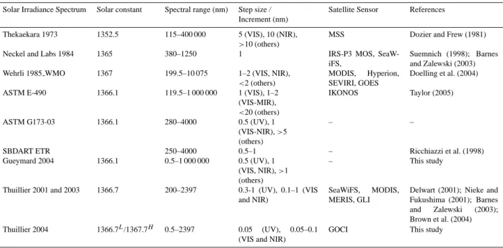
Table 1. Background of the applied solar irradiance spectra in various remote sensing applications.
Solar Irradiance Spectrum Solar constant Spectral range (nm) Step size /
Increment (nm)
Satellite Sensor References
Thekaekara 1973 1352.5 115–400 000 5 (VIS), 10 (NIR),
>10 (others)
MSS Dozier and Frew (1981)
Neckel and Labs 1984 1365 380–1250 1 IRS-P3 MOS,
SeaW-iFS,
Suemnich (1998); Barnes and Zalewski (2003)
Wehrli 1985 WMO 1367 199.5–10 075 1–2 (VIS, NIR),
<2 (others)
MODIS, Hyperion,
SEVIRI, GOES
Doelling et al. (2004)
ASTM E-490 1366.1 119.5–1 000 000 1 (VIS), 1–2
(VIS-MIR), <20 (others) IKONOS Taylor (2005) ASTM G173-03 1366.1 280–4000 0.5 (UV), 1 (VIS-NIR), >5 (others) – –
SBDART ETR 250–4000 0.5–1 – Ricchiazzi et al. (1998)
Gueymard 2004 1366.1 0.5–1 000 000 0.5 (UV), 1
(VIS, NIR), >1 (others)
– This study
Thuillier 2001 and 2003 1366.7 200–2397 0.3-1 (UV), 0.1–1 (VIS
and NIR)
SeaWiFS, MODIS,
MERIS, GLI
Delwart (2001); Nieke and Fukushima (2001); Barnes
and Zalewski (2003);
Brown et al. (2004)
Thuillier 2004 1366.7L/1367.7H 0.5–2397 0.05 (UV), 0.05–0.1
(VIS and NIR)
GOCI This study
* UV – Ultraviolet, VIS – Visible, NIR – Near infrared, MIR – Middle infrared, L – value for low-activity sun, H – value for high-activity sun.
Frew, 1981; Suemnich, 1998; S. Delwart, 20011; Nieke and Fukushima, 2001; Barnes and Zalewski, 2003; Doelling et al., 2004; Tayler, 2005). Most of them have been reported during 1973–2004 (Thekaekara, 1973; Neckel and Labs, 1984; Wehrli, 1985; Ricchiazzi et al., 1998 (SBDART ETR); ASTM, 2000 (E-490 and G173-03); Gueymard, 2004; Thuil-lier, 2004). These irradiance spectra are not monolithic, but rather composites of various spectra recorded by different instruments, in different spectral bands, with different res-olution and calibration methods, on different platforms, and at different moments in time. This is the reason why the applied irradiance spectra differ substantially depending on the sources of data in each waveband and resolution, various scaling factors and atmospheric correction procedures.
Table 1 presents the characteristics of various solar ir-radiance spectra adopted in Earth remote sensing applica-tions over the last three decades. During the early period, Thekaekara was instrumental in presenting some of his prim-itive AM0 (“air mass zero” extrapolation) irradiance spec-tra, obtained mostly from research aircrafts and rockets. The author performed considerable corrections and adjustments to compensate for all atmospheric interferences (chiefly by ozone and water vapour), in order to extrapolate irradiances to the top of the atmosphere and reconcile the various ra-diometric scales in effect. Though the composite spectrum was limited in spectral range and had large uncertainties
1Delwart, S.: ESA ESTEC, Keplerlan1, 2201 AZ Noordwijk
ZH, the Netherlands; personal communication, 2001.
from conventional techniques of extrapolation, it became the standard reference spectrum in calibrating early Land-sat MSS and other instruments (Dozier and Frew, 1981). In 1984, Neckel and Labs reported a composite solar spectrum from rockets (200–330 nm), high altitude observations (330– 1250 nm) and other sources (>1250 nm). Indeed, this spec-trum has been widely accepted for use in scientific applica-tions of many remote sensors, such as CZCS, IRS-P3 MOS and SeaWiFS (Suemnich, 1998; Barnes and Zalewski, 2003). In 1985, the World Meteorological Organization (WMO) of the World Radiometric Centre (WRC) constructed the Wehrli spectrum (AM0) as a composite of four existing data sets: rocket and balloon data (for 200–310 nm), scaled spectrum of Arvesen et al. (1969) (for 310–330 nm), Neckel and Labs (1981) (for 330–869 nm) and Smith and Gottlieb (1974) (for
>870 nm). Scaling and smoothening were performed in
or-der to match the resulting total irradiance with the solar con-stant 1367 W m−2 (see Table 1). Although such processes introduced noticeable errors in the resulted irradiance values, the Wehrli spectrum remains as the most cited spectrum in the literature and is considered as the reference for MODIS, SEVIRI, GOES and IKONOS sensors (Doelling et al., 2004). During the recent period, several satellites have been de-ployed in space to provide modern spectra, which com-bined with modeled data have rapidly improved the accu-racy over existing spectra. The American Society for Test-ing and Materials (ASTM) has published the ASTM G173-03 and ASTM E-490 (AM0) spectra, of these the former is
quite different from the standard solar spectrum as it repre-sents spectral irradiance on a surface of specified orientation under one set of specified atmospheric conditions. Such a measurement is often influenced by the absorption of large parts of the original solar spectrum by the Earth’s atmosphere which blocks or strongly attenuates most of the solar ultravi-olet (UV) and infrared radiation (Fligge and Solanki, 2000). In contrast, the latter one is based on data from satellites, space shuttle missions, high-altitude aircraft, rocket sound-ings, ground-based solar telescopes, and models. In the 119.5 to 410 nm range, the values are averages of two dif-ferent instruments on the UARS, SUSIM and SOLSTICE (Woods et al., 1996) (Table 2). In the 410 to 825 nm range, the values are from the McMath Solar Telescope at Kitt Peak, Arizona (Neckel and Labs, 1984). In the 825 to 4000 nm range, the values are from the high-resolution solar atlas computed by Kurucz (1984). Scaling and adjustment pro-cesses were also involved so that the integrated irradiance is equal to 1366.1 W m−2. The drawback with this spec-trum is that its resolution is limited to 1nm below 630 nm and 2 nm above it, which may not be adequate for applica-tions based on the new generation ocean colour missions. The SBDART (Santa Barbara DISORT Atmospheric Radia-tive Transfer) computes a solar irradiance spectrum based on the LOWTRAN-7 solar spectrum (Thekeakara, 1974) and a composite of information gathered by several different spec-tral measurement campaigns. The specspec-tral data collected from the Solar Ultraviolet Spectral Irradiance Monitor on Spacelab 2 (VanHoosier et al., 1988) are used for wave-lengths between 174 and 351 nm, while the observations of Neckel and Labs (1984) and Wehrli (1985) are used for wavelengths 351–868 nm and 868–3226 nm, respectively.
In 2004, Gueymard developed a more sophisticated syn-thetic solar spectrum, which uses vacuum wavelengths below 280 nm and air wavelengths above 280 nm, and is corrected for 1 ua (astronomical unit). Three resolutions and spectral intervals have been used in the construction of this spectrum, i.e. 0.5 nm in the UV (280–400 nm), 1nm in the visible (VIS) and near-infrared (NIR) (400–1702 nm), and 5 nm beyond, up to 4000 nm. This is a composite of the weighted average of twenty-three existing measured or modeled spectra from various sources and is constrained to 1366.1 W m−2. More recently, new experiments on various space platforms have been performed allowing an observation of the Sun without absorbing the influence of the Earth’s atmosphere, for ex-ample, the experiments with SOLSPEC spectrometers flown on all three missions of the NASA-sponsored ATLAS and EURECA (Thuillier, 2004). These three spectrometers of SOLSPEC monitor solar irradiance changes in the UV (180– 370 nm), VIS (350–900 nm) and IR (800–3000 nm) ranges with a spectral resolution of 1 nm each, offering the immense advantage of an exceptionally low uncertainty compared to all other experiments. The modern spectrum from these in-struments (for 29 March 1992 and 11 November 1994) has been recently released by Thuillier et al. (2004) (henceforth
Table 2. Glossary of experiments/instruments.
HF Hickey-Frieden cavity radiometer ACRIM Active Cavity Radiometer Irradiance
Monitor
SMM Solar Maximum Mission
ERBE Earth Radiation Budget Experiment ra-diometer
ERBS Earth Radiation Budget Satellite UARS Upper Atmosphere Research Satellite VIRGO Variability of solar IRradiance and
Grav-ity Oscillations
SOHO Solar and Heliospheric Observatory UARS Upper Atmosphere Research Satellite SUSIM Solar Ultraviolet Spectral Irradiance
Monitor
SOLSTICE SOLar STellar Irradiance Comparison Experiment
SOLSPE SOLar SPECtrum
ATLAS Atmospheric Laboratory for Application and Science
EURECA EUropean Retrievable Carrier
GOES Geostationary Operational Environmen-tal Satellites
MSS Multi Spectral Scanner
MOS Modular Optoelectronic Scanner SEVIRI Spinning Enhanced Visible and
Infra-Red Imager
MODIS Moderate-resolution Imaging Spectrora-diometer
GLI Global Line Imager
SeaWiFS SeaWiFS stands for Sea-viewing Wide Field-of-view Sensor
MERIS MEdium Resolution Imaging Spectrom-eter
GOCI Geostationary Ocean Colour Imager
“Thuillier 2004 spectrum”), which spans a wavelength range of 0.1 to 2400 nm with the highest spectral interval of 0.05– 0.1 nm. In fact, the previous versions of this spectrum (Ta-ble 1) have been recommended for use in the calibration and validation of MERIS and GLI (IOCCG report, 2003) and of SeaWiFS and MODIS (Brown et al., 2004).
This study presents a detailed evaluation of the above described solar irradiance spectra and examines the conse-quences of their disparities in ocean colour remote sensing. Because different solar irradiance models convert the same radiance or reflectance into different radiance or reflectance, the model-to-model differences are assessed in their abso-lute terms and in the in-band irradiances computed using the spectral response functions of SeaWiFS and MERIS’s channels, which are quite similar to those included in the design of the Geostationary Ocean Colour Imager (GOCI) scheduled for launch in 2008. The consequences of these differences on the retrieval algorithms of chlorophyll and
33 1363 1363.5 1364 1364.5 1365 1365.5 1366 1366.5 1367 1367.5 1368 1368.5 1369 1 9 7 6 0 1 0 1 1 9 7 7 0 5 1 5 1 9 7 8 0 9 2 7 1 9 8 0 0 2 0 8 1 9 8 1 0 6 2 2 1 9 8 2 1 1 0 4 1 9 8 4 0 3 1 8 1 9 8 5 0 7 3 1 1 9 8 6 1 2 1 3 1 9 8 8 0 4 2 6 1 9 8 9 0 9 0 8 1 9 9 1 0 1 2 1 1 9 9 2 0 6 0 4 1 9 9 3 1 0 1 7 1 9 9 5 0 3 0 1 1 9 9 6 0 7 1 3 1 9 9 7 1 1 2 5 1 9 9 9 0 4 0 9 2 0 0 0 0 8 2 1 2 0 0 2 0 1 0 3 2 0 0 3 0 5 1 8 2 0 0 4 0 9 2 9 2 0 0 6 0 2 1 1 Year/month/day T S I (W m -2 )
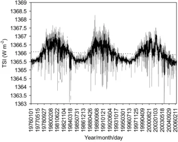
Fig. 1. The variation of total solar irradiance (TSI) during 1976–
2006. The solar constant obtained is 1366.1 W m−2. Data are from the HF on Nimbus 7, the ACRIM I on SMM, the ERBE on ERBS, the ACRIM II on UARS, the VIRGO on SOHO, and the ACRIM III on ACRIM-Sat (see Table 2).
suspended sediment are also assessed, and finally, an appro-priate irradiance spectrum is put forward for the GOCI de-velopment and for the future research and validation in ocean colour remote sensing.
2 The variation of solar spectral irradiance and the so-lar constant
The solar spectral irradiance fluctuates depending on the well documented 11-year solar cycle and also the Sun’s 27-day rotation cycle. It exhibits strong wavelength dependence with the amount of variability considerably increasing to-wards shorter wavelengths (Lean, 1991). In the ultravio-let (1–400 nm) the magnitude of irradiance variations is on the order of 1–14% and in the visible and NIR part of the spectrum (>400 nm) it is less than 1% (Fligge and Solanki, 2000). These variations in the solar irradiance spectrum are mainly caused by the effects of the facular brightening and sunspot darkening. While sunspots dominate short-term changes on time scales of a few days to weeks (Willson and Hudson, 1981), faculae and bright network elements are sup-posed to live much longer and therefore seem to contribute significantly to the variability of the solar cycle (Pap, 1998). The change in solar activity ultimately causes a variation in the total solar irradiance (TSI), which can be related to the spectral irradiance (Eo(λ)) through Eq. (1)
TSI = ∞
Z
0
Eo(λ)dλ. (1)
For studying the variations of TSI, several space-borne ra-diometers (e.g. the HF on Nimbus 7, the ACRIM I on SMM, the ERBE on ERBS, the ACRIM II on UARS, the VIRGO on SOHO, and the ACRIM III on ACRIM-Sat in Table 2) have been deployed to provide continuous measurements of solar irradiances on a daily basis since late November 1978 (Frohlich and Solanki, 2000; Pap et al., 2002). Because these instruments had a different calibration and degradation prob-lems, the overlapping data sets were originally not in per-fect quantitative agreement, even though they agreed qual-itatively in the shape and magnitude of the TSI variations during successive solar cycles. Therefore, researchers have made considerable efforts to reconcile time-limited TSI data sets and develop a unique composite time series from the best available data (Pap et al., 2002; Frohlich, 2004). Exam-ples of such a time series are the PMOD, IRMB and ACRIM (http://www.pmodwrc.ch/).
Figure 1 shows the most recent and extended PMOD TSI composite which consists of mean daily values, as well as a 27-day moving average (to dampen short-term ef-fects), together with amplitudes of the three cycles. Note that for interpolation, the data of 1976–1978 generated from empirical models are also included in this com-posite. It becomes obvious that the absolute minimum and maximum daily solar activity in terms of TSI are 1363 W m−2and 1368.3 W m−2for data sets of 1976–2006, and 1364.7 W m−2and 1367.2 W m−2for 27-day moving av-erage data sets. These data sets depict the solar constant (i.e. the long-term average of TSI) to be 1366.1 W m−2, and the variation of TSI by about 0.16% over the solar cycle, with 27-day amplitudes normally lower than 11-year amplitudes (Fig. 1). This new solar content is very essential for an im-proved approximation of the extraterrestrial solar spectrum in the UV- NIR region.
3 The function of solar irradiance in ocean colour re-mote sensing
Since most of the Earth’s imaging spectrometers are not de-signed to provide calibrated solar irradiances, knowledge of the absolute spectral values of solar irradiance is required for measurements of the ocean colour from space and in-situ. These values are constant during time and primarily go into the process of radiometric calibration, atmospheric correc-tion algorithms and normalizacorrec-tion of water-leaving radiances from in-situ measurements. Radiometric calibration refers to the mapping between instrument response in digital counts and the radiance at the instrument aperture. It is common to define a mean spectral radiance on the basis of measured in-band radiance in Eq. (2)
Li = Li ψi = ∞ R 0 φ (λ)L(λ)dλ ∞ R 0 φ (λ)dλ , (2)
where Li is the mean spectral radiance, Li is the in-band ra-diance integrated over the spectral bandpass of the relevant channel, φ (λ) is the instrument spectral response function,
L(λ) is the spectral radiance at the instrument aperture, and ψi is the effective width of the spectral bandpass. This radi-ance may be further expressed as a reflectradi-ance factor, defined as the ratio of the upwelling radiance over a lambertian sur-face that would produce the measured in-band radiance, to the irradiance of the extraterrestrial solar beam, as follows,
Ri =
π Li
Eio , (3)
where Ri is the reflectance factor and Eiois the extraterres-trial solar irradiance integrated over the spectral bandpass of channel i. It is important to distinguish the reflectance factor from the top of the atmosphere directional reflectance (Ri) through, Ri = π Li Eoi cos θs = π Li Eoi(1 AU)r−2cos θ s , (4)
where cos θsis the solar zenith angle. Note that, for constant in-band radiance the reflectance factor varies during the year, owing to the ellipticity of the Earth’s orbit about the Sun. This seasonal variation can be expressed by Eio(1 AU)r−2, where Eio(1 AU) is the in-band extraterrestrial solar irradi-ance at one astronomical unit (AU), which is the norm, and
r−2is the Sun-Earth distance in AU.
The above term recorded by a satellite sensor at the level of the top of the atmosphere (TOA) is the total reflectance comprising of the complex atmospheric path reflectance, sea surface reflectance and water-leaving reflectance. About 80– 90% of the total signal results from the atmosphere and sea surface, while the remaining part results from the near-surface waters of the ocean. This small part carries immense information concerning the ocean biogeochemical variables, including the concentration of phytoplankton which consti-tutes the first link in the marine food chain. The process of removing the large part of the undesired (atmospheric and sea surface) signal is denoted as an atmospheric correction, which derives the fundamental quantity of water-leaving re-flectance that can be related to the optical properties of the water body (i.e. to the substance in it). In remote sensing of the ocean colour, the important, time-independent quantity is the normalized water-leaving radiance [nLw(λ)] which is used in the derivation of in-water algorithms and the estima-tion of sea water constituents from satellite data. According to Gordon and Clark (1981), the nLw(λ) can be obtained by dividing the water-leaving radiance [Lw(λ)] by the down-welling irradiance just above the surface [Ed(0+λ)], and then
multiplying it by the mean extraterrestrial solar irradiance [Eo(λ)] at the TOA, as in Eq. (5),
nLw(λ) = [Lw(λ)/Ed(0+λ)] × Eo(λ). (5) In this equation, ignoring Eo(λ) yields the remote sensing reflectance [Rrs(0+λ)] that is directly related to the inher-ent optical properties (IOP) of water and substances within it (Ahn et al., 2001) and used to calculate many other quanti-ties related to ocean optics. In the case of in-situ field mea-surements, both Lw(λ) and Ed(0+λ) can be obtained with field radiometers at the sea. But for satellite sensors that do not measure Ed(0+λ), this term is instead computed through Eq. (6)
Ed(0+λ) = Eo(λ)r−2cos(θs)td(λ, θs), (6) where cos θs is the solar zenith angle and td(λ, θs) is the at-mospheric diffuse transmittance in the solar direction with the solar zenith angle of θs. By introducing this term into Eq. (5) and accounting for the dependency upon the geomet-rical conditions of satellite observation, one can obtain the satellite-derived normalized water-leaving radiance as fol-lows,
nLw(λ, θs, θv, 1ϕ) =
Lw(λ, θs, θv, 1ϕ)/r−2cos(θs)td(λ, θs), (7) where θvis the viewing angle and 1ϕ is the azimuth differ-ence between the solar plane and the plane of observation. Here the satellite observed nLw(λ, θs, θv, 1ϕ) values are in-dependent of the choice of Eo(λ), which is used twice in the calculation, thereby canceling out the spectrum by virtue of the normalization. However, this is not the same case with the in-situ measurement of upwelled radiance, which depends on the choice of Eo(λ) while transforming into
nLw(λ).
On the other hand, the irradiance reflectance is an appar-ent optical property defined as the ratio of upwelling irra-diance [Eu(0−, λ)] to downwelling irradiance [Ed(0−, λ)], both spectral irradiances are ideally determined at null depth (0−). Its spectral value from Ahn et al. (2001) is given in
Eq. (8), R(0−, λ) = Eu(0 −, λ) Ed(0−, λ) = QuLu(0 −, λ, θ, 1ϕ) (1 − ρ)Ed(0+, λ) . (8)
This quantity essentially depends on the water optical prop-erties and also on illumination conditions. In this equation,
Lu(0−, λ, θ, 1ϕ) is the upwelling radiance in the direction of zenith (θ ) and azimuth (1ϕ) angles just beneath the sur-face. In the conversion of Ed(0−, λ) to Ed(0+, λ), ρ is used, which is the Fresnel reflectance at the air-sea inter-face for the whole (Sun + sky) downwelling irradiance, typ-ically amounting to within the range of 4–5% (Morel and Gentili, 1996). It also varies with the sea surface state (wind speed). The Qufunction (the ratio of upwelling irradiance to
34
Fig. 2. The spectral response functions (unitless) of SeaWiFS and MERIS superimposed on the Thuillier
µ MERIS -2500 -2250 -2000 -1750 -1500 -1250 -1000 -750 -500 -250 0 250 500 750 1000 1250 1500 1750 2000 2250 2500 3 5 0 4 0 0 4 5 0 5 0 0 5 5 0 6 0 0 6 5 0 7 0 0 7 5 0 8 0 0 8 5 0 9 0 0 9 5 0 1 0 0 0 1 0 5 0 1 1 0 0 1 1 5 0 1 2 0 0 Wavelength (nm) S p e c tr a l I rr a d ia n c e ( W m -2 µ m -1) -1 -0.9 -0.8 -0.7 -0.6 -0.5 -0.4 -0.3 -0.2 -0.1 0 0.1 0.2 0.3 0.4 0.5 0.6 0.7 0.8 0.9 1 SeaWiFS N o rm a lize d sp ce tr a l r e sp o n se ( u n itl e s s)
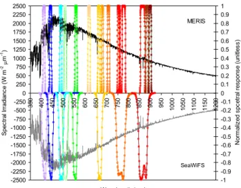
Fig. 2. The spectral response functions (unitless) of SeaWiFS and
MERIS superimposed on the Thuillier 2004 irradiance spectrum (W m−2µm−1). To avoid overlapping of the spectral response
functions of SeaWiFS and MERIS, each one is displayed on either side of this plot.
upwelling radiance, (Eu(0−, λ)/Lu(0−, λ), in units of stera-dians) is not a constant but a function of depth and direction (θ , 1ϕ). The R(0−, λ) quantity can be linked to the
normal-ized water-leaving radiance through Eq. (9) given by Morel and Gentili (1996),
nLw(λ, θs, θv, 1ϕ) = Eo(λ)R(0−, λ, θs)ℜ(λ, θvW )/
Qu(λ, θsθv1ϕ), (9) where ℜ is a dimensionless quantity equal to 0.529 (Gor-don, 2005), as long as θv<40◦(Morel and Belanger, 2006). This quantity combines all the effects of reflection and re-fraction at the air-sea interface and becomes slightly depen-dent on the sea state (wind speed). The derived nLw quan-tity is largely independent of the time of day when mea-surements are made. Because of this and of the signifi-cant dependence on the concentrations of material in the water column, many bio-optical algorithms developed in re-cent years rely on this quantity to retrieve the accurate infor-mation of optically-active constituents (such as the surface concentration of phytoplankton) from satellite measurements in ocean waters (e.g. M¨uller-Karger et al., 1990; McClain and Yeh, 1994; Aiken et al., 1995; O’Reilly et al., 1998; Ahn et al., 2001; Darecki and Stramski, 2004; Morel and Belanger, 2006; Bailey and Werdell, 2006; Ahn and Shan-mugam, 2006).
4 Major ocean colour missions – SeaWiFS, MERIS and GOCI
This study considers two major imaging spectrometers, Sea-WiFS and MERIS, whose spectral characteristics are quite similar to those of the GOCI proposed by the Korea Ocean Research and Development Institute (KORDI). These imag-ing spectrometers have the capability of providimag-ing an impor-tant advantage in studying and understanding the processes at scales of continental shelves and coastal seas. The Sea-WiFS, flown on the Orbview-2 SeaStar satellite on a Sun-synchronous orbit (at 705 km) in August 1997 by the Na-tional Aeronautics and Space Administration (NASA), pro-vides near-global coverage every 2 days of upwelled radi-ance for eight narrow spectral channels (nm) in the visible and near-infrared spectral domain, with the spatial resolution of ∼1 km/pixel at nadir. The special features of this instru-ment are that its bands have a bilinear gain response to enable them to avoid saturation over most land and cloud features, it can be tilted to −20, 0, or +20 degrees to avoid Sun glint reflecting off the oceans, and the resultant data rounded to 10 bit numbers provide high quality information on varying water constituents. On the other hand, the MERIS, flown on its Envisat Earth Observation Satellite (ENVISAT-1) on a Sun-synchronous orbit (at 799.8 km) in March 2002 by the European Space Agency (ESA), measures the upwelled radi-ance for 15 spectral bands in the 412–900 nm spectral range. It possesses a high spatial (300 m), spectral, and radiomet-ric resolution (accuracy from 400 to 900 nm<2% and from 900 to 1050 nm<5%), covering the open ocean and coastal waters with a swath of 1150 km (Bezy et al., 2000).
In comparison with open ocean applications, coastal ap-plications involving phenomena that vary on shorter space and time scales demand a simultaneous increase in spa-tial and temporal resolution. To provide an important new capability for imaging the coastal zone, the GOCI is de-signed to be operated in a staring-frame capture mode on board its Communication Ocean and Meteorological Satel-lite (COMS) and is tentatively scheduled for launch in 2008. The mission concept includes eight visible-to-near-infrared bands, a 500 m×500 m pixel resolution, and a coverage re-gion of 2500 m×2500 km centered at 36 N and 130 E (KO-RDI report, 2003). The GOCI will provide multiple views of many locations within the fixed region during a single day (i.e. 8 images during the daytime and 2 images during the nighttime) that would help in detecting and monitoring the red tide algal blooms, river plumes and other circulating pat-terns in the vicinity of the coast. Table 3 provides a com-parison between the spectral characteristics of the SeaWiFS, MERIS and GOCI sensors.
Figure 2 displays the normalized spectral response func-tions (unitless) of SeaWiFS and MERIS superimposed on the Thuillier 2004 irradiance spectrum in the ultraviolet to NIR domain (350–1200 nm). The SeaWiFS response functions are given at wavelength intervals of 1 nm (from 400–900 nm)
and the MERIS response functions are given at wavelength intervals of close to 0.1 nm. Note that, the MERIS spectral bands have almost half the spectral widths of the SeaWiFS bands and their response functions and peaks are narrower and smoother than those of SeaWiFS, which exhibits the lack of smoothness in the peaks of the curves for band 7 (765 nm) and 8 (865 nm). This may be related to an artifact of the mea-surement of the band’s interference filter designed for SeaW-iFS (Hooker et al., 1994). The peak-normalized spectral re-sponse functions are input into the model for computing the in-band irradiances of these sensors.
5 Results
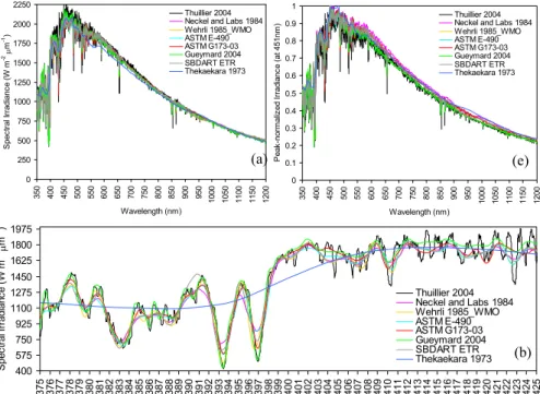
5.1 The solar irradiance spectra and their differences An exhaustive survey of this study reveals a variety of exist-ing data sets coverexist-ing the diverse spectral ranges, instrumen-tal sources and measurements periods. Among these data sets only eight irradiance spectra are chosen for this inves-tigation, namely the Thuillier 2004, Neckel and Labs 1984, Wehrli 1985 WMO, ASTM E-490, ASTM G173-03, Guey-mard 2004, SBDART ETR, and Thekaekara 1973. Figure 3a displays these eight spectra that vary with wavelength, ris-ing near the green and droppris-ing gradually toward the NIR and abruptly toward the UV part of the spectrum. Fig-ures 3b–d better illustrate the model-to-model differences and the strength and weakness of each of them in the UV, VIS (blue-green) and NIR domains. This intercomparison en-ables us to identify four types of problems, i.e. localized inac-curacy around a specific wavelength, band underestimations or overestimations, a sharp underestimation structure corre-sponding to atmospheric absorption interference in uncor-rected data (particularly in the NIR), and rapid wavelength-to-wavelength fluctuations close to solar Fraunhofer lines (after Joseph von Fraunhofer in 1814) and other solar absorp-tion features caused by a slight spectral shift between spectra (particularly in the UV, VIS and NIR). It should be noted that the latter experimental problem induces important spikes in the relative differences among these spectra from 350 nm to 1000 nm, mainly due to the abundance of sharp structures related to Fraunhofer and other absorption lines (Gueymard, 2004). These lines are generally observed as dark features in the solar spectrum and include the L line of Fe at 383 nm, the K line of Ca II at 393.4 nm, the H line of Ca II at 396.8 nm, the h line of Hδ at 410.2 nm, the G line of Ca at 430.7 nm, the G line of Fe at 430.8 nm, the G′line of Hγ at 434 nm, the e line of Fe at 438.35 nm, the d line of Fe at 466.8 nm, the F line of Hβ at 486.3 nm, the c line of Fe at 495.7 nm, the b4 line of Mg at 516.73 nm, the b4 line of Fe at 516.75 nm, the b3 line of Fe at 516.9 nm, the b2 line of Mg at 517.27 nm, the b1 line of Mg at 518.3 nm, the E2line of Fe at 527 nm, the
D3line of He at 587.56 nm, the D2line of Na at 588.9 nm,
the D1line of Na at 589.6 nm, the C line of Hα at 656.3 nm,
and other absorption lines at 850, 854 and 866 nm. Besides these lines, there are also the Earth’s telluric absorption lines related to molecular oxygen (O2), carbon monoxide (CO),
and other molecules that contribute particularly to the NIR. Consider the Thuillier 2004 spectrum, because of its high spectral resolution all major Fraunhofer lines seem to be deeper and narrower than those in other spectra. In the cases of Gueymard 2004, ASTM E-490 and ASTM G173-03 spectra, the absorption lines are quite identical in shape and depth though their spectral positions deviate slightly from the Thuillier 2004 spectrum. In contrast, the Neckel and Labs 1984, Wehrli 1985 WMO and SBDART ETR spectra show the spectrally shifted, reduced lines at these specific wave-lengths and the Thekaekara 1973 irradiance does not bring this variability to our observation, owing to its limited spec-tral resolution. Perhaps the change in solar activity could also cause such differences around the Fraunhofer lines (Guey-mard, 2004).
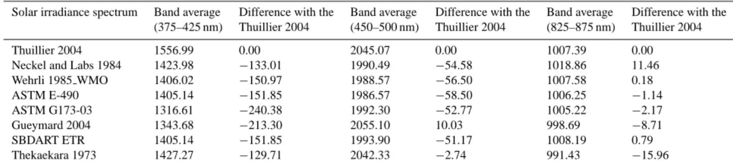
Not surprisingly, the large differences are also observed among eight irradiance spectra in the three plots of UV (375–425 nm), VIS (450–500 nm) and NIR (825–875 nm) (Figs. 3b–d). These differences increase from the NIR to VIS and become very prominent in the UV region. To bet-ter illustrate the magnitude of these differences, the irradi-ance values of each reference spectrum are averaged for the above wavelength ranges and the differences with the Thuil-lier 2004 spectrum (taken as the reference because it rep-resents the current state of the art in solar irradiance spec-tra of exceptionally low uncertainty compared to others; Rottman et al., 2004) are calculated and given in Table 4. In both the absolute and band-averaged terms (W m−2µm−1),
the Thuillier 2004 spectrum is relatively higher in the UV and VIS and shows consistency with other spectra in the NIR (except Fraunhofer lines). While taking the differ-ence with the Thuillier 2004 spectrum, the Gueymard 2004 spectrum seems to be closer to the Thuillier 2004 spectrum at 450–500 nm, but differs substantially by −213.30 and
−8.71 W m−2µm−1 at 375–425 nm and 825–875 nm, re-spectively. The Thekaekara 1973 spectrum, though exhibit-ing relatively less of a difference at UV and VIS (blue), yields a large negative difference with the Thuillier 2004 at NIR (the absolute term also explains this difference seen from 500–900 nm). The differences in the Wehrli 1985 WMO, ASTM E-490 and SBDART ETR spectra are generally less at 825–875 nm (0.18, −1.14 and 0.79 W m−2µm−1, respectively), but are significant at 450–500 nm (−56.50,
−58.50 and −51.17 W m−2µm−1, respectively) and 375–
425 nm (−150.97, −151.85 and −151.85 W m−2µm−1,
re-spectively). Among the ASTM G173-03 and Neckel and Labs 1984 spectra, the ASTM G173-03 appears to be closer to the Thuillier 2004 than the Neckel and Labs 1984 at 825–875 nm and 450–500 nm. However, at 375–425 nm the situation becomes reversed, i.e. the ASTM G173-03 differs by a factor of −240.38 W m−2µm−1 larger than
Table 3. The characteristics of SeaWiFS, MERIS and GOCI sensors.
Centre Wavelength ± Bandwidth(nm) Application/mission objectives
SeaWiFS MERIS GOCI
412±20 412.5±10 412±20 Yellow substance and detrital matter 443±20 442.5±10 443±20 Chlorophyll absorption maximum 490±20 490±10 490±20 Chlorophyll and other pigments 510±20 510±10 Suspended sediment, red tides
555±20 560±10 555±20 Chlorophyll reference, suspended sediments
620±10 Suspended sediments
670±20 665±10 660±10 Chlorophyll absorption and fluorescence base 1 681.25±7.5 680±10 Chlorophyll fluorescence peak
708.7 5±10 Atmospheric correction, fluorescence base 2 753.75±7.5 Vegetation, cloud
765±40 760.625 ±3.75 745±20 Chlorophyll fluorescence base 2, Oxygen absorption (in case of MERIS) 778.75±15 Atmospheric correction, vegetation
865±40 865±20 865±40 Water vapour reference, vegetation 885±10 Atmospheric correction
900±10 Water vapour, land
Table 4. The band-averaged values and their differences with the Thuillier 2004 spectrum.
Solar irradiance spectrum Band average Difference with the Band average Difference with the Band average Difference with the (375–425 nm) Thuillier 2004 (450–500 nm) Thuillier 2004 (825–875 nm) Thuillier 2004
Thuillier 2004 1556.99 0.00 2045.07 0.00 1007.39 0.00
Neckel and Labs 1984 1423.98 −133.01 1990.49 −54.58 1018.86 11.46
Wehrli 1985 WMO 1406.02 −150.97 1988.57 −56.50 1007.58 0.18 ASTM E-490 1405.14 −151.85 1986.57 −58.50 1006.25 −1.14 ASTM G173-03 1316.61 −240.38 1992.30 −52.77 1005.22 −2.17 Gueymard 2004 1343.68 −213.30 2055.10 10.03 998.69 −8.71 SBDART ETR 1405.14 −151.85 1993.90 −51.17 1008.19 0.79 Thekaekara 1973 1427.27 −129.71 2042.33 −2.74 991.43 −15.96
Figure 3e better illustrates the differences in these eight spectra, normalized by the peak value at 451 nm. The ob-served differences are indeed much higher than the 0.16% of the solar-induced variability in the UV-NIR domain and can be related to the instrumental uncertainty and calibration problems, and ineffective atmospheric correction procedures.
5.2 The SeaWiFS and MERIS in-band solar irradiances and their differences
The Earth observation sensors, like SeaWiFS and MERIS, do not carry independent devices to provide calibrated solar ir-radiances to transform their measurements to reflectances at the TOA. Consequently, they depend on a single solar irra-diance spectrum from instruments specifically designed for measuring the Sun. Because different irradiance spectra con-vert the TOA signal into different reflectances, this study ju-diciously examines the model-to-model differences in terms of the in-band irradiances (Eio), computed using the spectral
response functions of SeaWiFS and MERIS’s channels, as follows, Eoi = ∞ R 0 φ (λ)Eo(λ)dλ ∞ R 0 φ (λ)dλ , (10)
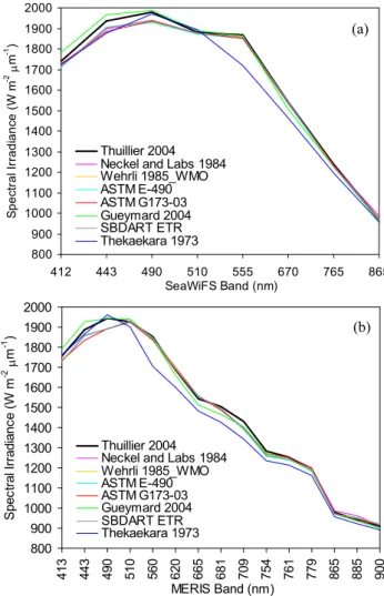
where φ (λ) is the relative spectral response of the SeaWiFS or MERIS’s channel (i), and Eo(λ) is the spectral irradiance from different models interpolated to the wavelength inter-val of 1 nm and 0.1 nm for the SeaWiFS and MERIS spectral responses, respectively. Figures 4a and b depict the charac-teristics of the eight solar irradiances with partially or com-pletely removed Fraunhofer lines after being transformed into the SeaWiFS and MERIS’s in-band irradiances. As was noted before, the large differences exist between them, par-ticularly in the UV-VIS (412–510 nm), where the Gueymard 2004 spectrum is higher followed by the Thuillier 2004 and other spectra.
35 0 250 500 750 1000 1250 1500 1750 2000 2250 3 5 0 4 0 0 4 5 0 5 0 0 5 5 0 6 0 0 6 5 0 7 0 0 7 5 0 8 0 0 8 5 0 9 0 0 9 5 0 1 0 0 0 1 0 5 0 1 1 0 0 1 1 5 0 1 2 0 0 Wavelength (nm) S p e c tr a l Ir ra d ia n c e ( W m -2 µ m -1) Thuillier 2004 Neckel and Labs 1984 Wehrli 1985_WMO ASTM E-490 ASTM G173-03 Gueymard 2004 SBDART ETR Thekaekara 1973 0 0.1 0.2 0.3 0.4 0.5 0.6 0.7 0.8 0.9 1 3 5 0 4 0 0 4 5 0 5 0 0 5 5 0 6 0 0 6 5 0 7 0 0 7 5 0 8 0 0 8 5 0 9 0 0 9 5 0 1 0 0 0 1 0 5 0 1 1 0 0 1 1 5 0 1 2 0 0 Wavelength (nm) P e a k -n o rm a liz e d I rr a d ia n c e ( a t 4 5 1 n m ) Thuillier 2004 Neckel and Labs 1984 Wehrli 1985_WMO ASTM E-490 ASTM G173-03 Gueymard 2004 SBDART ETR Thekaekara 1973 (e) (a) 650 700 750 800 850 900 950 1000 1050 1100 1150 8 2 5 8 2 6 8 2 7 8 2 8 8 2 9 8 3 0 8 3 1 8 3 2 8 3 3 8 3 4 8 3 5 8 3 6 8 3 7 8 3 8 8 3 9 8 4 0 8 4 1 8 4 2 8 4 3 8 4 4 8 4 5 8 4 6 8 4 7 8 4 8 8 4 9 8 5 0 8 5 1 8 5 2 8 5 3 8 5 4 8 5 5 8 5 6 8 5 7 8 5 8 8 5 9 8 6 0 8 6 1 8 6 2 8 6 3 8 6 4 8 6 5 8 6 6 8 6 7 8 6 8 8 6 9 8 7 0 8 7 1 8 7 2 8 7 3 8 7 4 8 7 5 Wavelength (nm) S p e c tr a l Ir ra d ia n c e ( W m -2 µ m -1) Thuillier 2004 Neckel and Labs 1984 Wehrli 1985_WMO ASTM E-490 ASTM G173-03 Gueymard 2004 SBDART ETR Thekaekara 1973 1375 1475 1575 1675 1775 1875 1975 2075 2175 2275 4 5 0 4 5 1 4 5 2 4 5 3 4 5 4 4 5 5 4 5 6 4 5 7 4 5 8 4 5 9 4 6 0 4 6 1 4 6 2 4 6 3 4 6 4 4 6 5 4 6 6 4 6 7 4 6 8 4 6 9 4 7 0 4 7 1 4 7 2 4 7 3 4 7 4 4 7 5 4 7 6 4 7 7 4 7 8 4 7 9 4 8 0 4 8 1 4 8 2 4 8 3 4 8 4 4 8 5 4 8 6 4 8 7 4 8 8 4 8 9 4 9 0 4 9 1 4 9 2 4 9 3 4 9 4 4 9 5 4 9 6 4 9 7 4 9 8 4 9 9 5 0 0 Wavelength (nm) S p e c tr a l I rr a d ia n c e ( W m -2 µ m -1) Thuillier 2004 Neckel and Labs 1984 Wehrli 1985_WMO ASTM E-490 ASTM G173-03 Gueymard 2004 SBDART ETR Thekaekara 1973 (c) 400 575 750 925 1100 1275 1450 1625 1800 1975 3 7 5 3 7 6 3 7 7 3 7 8 3 7 9 3 8 0 3 8 1 3 8 2 3 8 3 3 8 4 3 8 5 3 8 6 3 8 7 3 8 8 3 8 9 3 9 0 3 9 1 3 9 2 3 9 3 3 9 4 3 9 5 3 9 6 3 9 7 3 9 8 3 9 9 4 0 0 4 0 1 4 0 2 4 0 3 4 0 4 4 0 5 4 0 6 4 0 7 4 0 8 4 0 9 4 1 0 4 1 1 4 1 2 4 1 3 4 1 4 4 1 5 4 1 6 4 1 7 4 1 8 4 1 9 4 2 0 4 2 1 4 2 2 4 2 3 4 2 4 4 2 5 Wavelength (nm) S p e c tr a l I rr a d ia n c e ( W m -2 µ m -1) Thuillier 2004 Neckel and Labs 1984 Wehrli 1985_WMO ASTM E-490 ASTM G173-03 Gueymard 2004 SBDART ETR Thekaekara 1973 (b) (d)
Fig. 3. (a) The spectral irradiance of the eight reference spectra in the UV to NIR (from 350–1200 nm) domains, (b–d) their magnified
portions in the ultraviolet-blue-green and NIR, and (e) the peak-normalized irradiance values (at 451 nm) in the 350–1200 nm range.
Figures 5a and b provide an assessment of the percent differences between the Thuillier 2004 and other spectra in the SeaWiFS and MERIS channels. In the case of Sea-WiFS (Fig. 5a), the difference in the Gueymard 2004 is at a minimum of 0.24% at 555 nm and at a maximum of
−2.21% at 412 nm, whereas in the Neckel and Labs 1984, Wehrli 1985 WMO, ASTM E-490, ASTM G173-03 and SB-DART ETR the differences are in the range of −0.90–0.11% at 865 nm and 1.38–2.51% at 443 nm (and slightly lower
0.57–1.47% at 412 nm). Such large differences in the 412 and 443 nm regions of major spectral lines (h line of Hδ at 410.2 nm and e line of Fe at 438.35 nm) can be tentatively explained by changes in the solar activity, uncertainties in the experimental data and spectral resolution of data. The Thekaekara 1973 spectrum shows the progressively high dif-ferences of 2.87% at 443 nm and 0.7–7.64% at NIR, which confirms the previous findings by Frohlich (1983). In the case of MERIS that includes several narrow and additional
1244 P. Shanmugam and Y. H. Ahn: Reference solar irradiance spectra
36
. 4a and b. The in-band irradiances for SeaWiFS (a) and MERIS (b).
800 900 1000 1100 1200 1300 1400 1500 1600 1700 1800 1900 2000 4 1 3 4 4 3 4 9 0 5 1 0 5 6 0 6 2 0 6 6 5 6 8 1 7 0 9 7 5 4 7 6 1 7 7 9 8 6 5 8 8 5 9 0 0 MERIS Band (nm) S p e c tr a l I rr a d ia n c e ( W m -2 µ m -1 ) Thuillier 2004 Neckel and Labs 1984 Wehrli 1985_WMO ASTM E-490 ASTM G173-03 Gueymard 2004 SBDART ETR Thekaekara 1973 (b) 800 900 1000 1100 1200 1300 1400 1500 1600 1700 1800 1900 2000 412 443 490 510 555 670 765 865 SeaWiFS Band (nm) S p e c tr a l Ir ra d ia n c e (W m -2 µ m -1 ) Thuillier 2004 Neckel and Labs 1984 Wehrli 1985_WMO ASTM E-490 ASTM G173-03 Gueymard 2004 SBDART ETR Thekaekara 1973 (a)
Fig. 4. The in-band irradiances for SeaWiFS (a) and MERIS (b).
channels, the above differences are further magnified and the new peaks and valleys appear to be prominent at 620, 681, 709, 754, 779, 885 and 900 nm (Fig. 5b). Perhaps a portion of this magnification in the differences of the in-band irra-diance spectra can be explained by several absorption lines close to the MERIS channels in the UV-NIR region (partic-ularly 412, 443, 490, 665 and 865 nm). Consider the Guey-mard 2004 spectrum, the percent differences with the Thuil-lier 2004 spectrum are small at 0.81–1.13% in the NIR chan-nels (754–900 nm) but significantly larger in the blue (413 and 443 nm) and red (620–709 nm) channels. This may be at-tributable to an inappropriate scaling factor applied to lessen the difference of its spectral irradiance with other sources of data and differences in the calibration between various mea-surements. The differences (minimal and maximal) in the Neckel and Labs 1984, Wehrli 1985 WMO, ASTM E-490, ASTM G173-03, and SBDART ETR spectra are of the or-der of −1.6–5.24%, −1.26–5.07%, −1.36–5.27%, −1.25– 5.35% and −1.52–5.10%. This is in contrast with −1.83– 14.6% for the Thekaekara 1973 spectrum which highly fluc-tuates with the Thuillier 2004 at wavelengths above 510 nm.
37 -3 -2 -1 0 1 2 3 4 5 6 7 8 9 412 443 490 510 555 670 765 865 SeaWiFS Band (nm) P e rc e n t d if fe re n c e f ro m T h u ill ie r 2 0 0 4 Thuillier 2004 Neckel and Labs 1984 Wehrli 1985_WMO ASTM E-490 ASTM G173-03 Gueymard 2004 SBDART ETR Thekaekara 1973 (a) -4 -2 0 2 4 6 8 10 12 14 16 18 413 443 490 510 560 620 665 681 709 754 761 779 865 885 900 MERIS Band (nm) P e rc e n t d if fe re n c e f ro m T h u ill ie r 2 0 0 4 Thuillier 2004 Neckel and Labs 1984 Wehrli 1985_WMO ASTM E-490 ASTM G173-03 Gueymard 2004 SBDART ETR Thekaekara 1973 (b)
Fig. 5. The percent differences between the Thuillier 2004 and other
spectra in SeaWiFS and MERIS channels.
Table 5 gives the band-averaged percent differences be-tween the Thuillier 2004 and other spectra in the SeaWiFS and MERIS channels. Overall, the differences in the Guey-mard 2004 spectrum are radically small when comparing with the others. Among the older spectra, the Neckel and Labs 1984 and SBDART ERT closely resemble each other in the differences with the Thuillier 2004, and the Wehrli 1985 WMO is slightly higher but reasonable when compar-ing with the ASTM G173-03 and ASTM E-490 spectra. The Thekaekara 1973 spectrum claims inaccuracy due to the in-clusion of terrestrial absorption features resulting from air-craft measurements.
5.3 The in-situ radiometric measurements and normaliza-tion
The extraterrestrial solar irradiance spectrum is involved in the process of transforming sea-truth (in-situ) mea-surements of water-leaving radiance (Lw) into normalized water-leaving radiance (nLw) and subsequently predicting
Table 5. The band-averaged percent differences with the Thuillier 2004 spectrum.
Sensor Neckel and Labs 1984 Wehrli 1985 WMO ASTM E-490 ASTM G173-03 Gueymard 2004 SBDART ETR Thekaekara 1973
MERIS 0.987845 1.112088 1.272651 1.198229 0.677517 0.97962 4.416144
SeaWiFS 0.719042 0.886044 0.975329 0.870834 −0.21814 0.728499 2.221714
the retrieval algorithms of the sea water constituents. To an-alyze the impact of the irradiance differences on these pro-cesses, the radiometric measurements of downward spectral irradiance Ed (λ), total water leaving radiance tLw(λ) and sky radiance Lsky(λ) collected during the period 1998–2004
of R/V (Research Vessel) Olympic cruises in the Korean South Sea (KSS) and Korean Southwest Sea (KSWS), R/V EARDO cruises in the East Sea (ES) and East China Sea (ECS), and R/V TAMGU cruises in the Yellow Sea, were processed. These measurements were performed at various sample sites using an ASD FieldSpec Pro Dual VNIR Spec-troradiometer with a spectral range from 350–1050 nm and a spectral sample interval of 1.4 nm. This instrument was cal-ibrated and several inter-calibrations with other instruments were performed to confirm its stability. The data recorded in units of mW cm−2µm−1sr−1were corrected for the contri-bution of skylight reflection and air-sea interface effects, in order to obtain Lw(λ)=t Lw(λ)−Fr(λ)×Lsky(λ), where the
Fr value was kept equal to 0.025 (Austin, 1974), in spite of its variability with viewing geometry, sky conditions and sea surface roughness due to wind (Mobley, 1999). For all the cruises, the concentrations of chlorophyll (Chl), suspended sediment (SS) and dissolved organic matter (DOM) were de-termined based on the standard spectrophotometric proce-dures and oven-drying method (Jeffrey and Humphrey, 1975; Ahn et al., 2001).
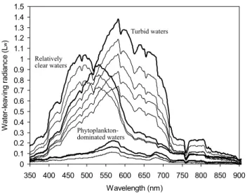
Figure 6 shows an example of the water-leaving radi-ance spectra collected in phytoplankton-dominated, turbid and relatively clear waters of the KSS, KSWS and south-ern YS during September 2002, February 2003 and August 2003. In highly turbid KSWS waters containing Chl=0.6– 1.6 mg m−3, SS=13–25 g m−3 and DOM=1.2–1.8 m−1, the
Lw spectra progressively increase with increasing turbid-ity and show three prominent peaks around 550–600 nm, 625–675 and 760–820 nm, attributable to the enhancement of backscattering by SS. The low Lw values in the shorter wavelength domain may be caused by the enhancement of absorption by weakly coloured sediment particles. In relatively clear YS waters containing Chl=0.8–1.2 mg m−3, SS=1.5–6 g m−3 and DOM=0.14–0.25 m−1, the Lw values are slightly high in the green and blue and low in the red and near-infrared wavelengths because of profound absorption by the seawater. In phytoplankton-dominated KSS waters con-taining Chl=12–21 mg m−3, SS=7–11 g m−3and DOM=0.5– 0.7 m−1, the weak Lw signals in the lower green and blue
are due to the combined absorption by phytoplankton pig-ments, DOM and other non-living suspended matters, and the strong Lw signals in the green and red wavelengths are due to the minimal total absorption and chlorophyll-a fluo-rescence (Morel and Prieur, 1977; Gitelson et al., 1994; Ahn et al., 2001).
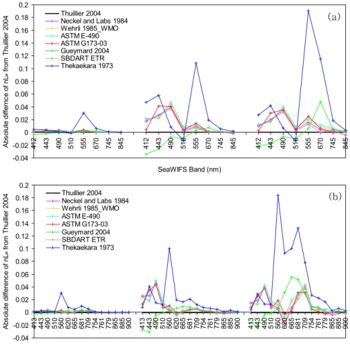
While the different Eo(λ) spectra were adopted to trans-form measurements of Lw into nLw in the SeaWiFS and MERIS channels, the differences observed were notably high, particularly in turbid and relatively clear waters (Figs. 7a and b). In phytoplankton-dominated waters, the absolute nLw differences between the Thuillier 2004 and other spectra (Neckel and Labs 1984, Wehrli 1985 WMO, ASTM E-490, ASTM G173-03, SBDART ETR and Guey-mard 2004) are within ±0.01. The Thekaekara 1973 has as expected a large difference with the Thuillier 2004 spec-trum, particularly at 555 nm and 560 nm. In the case of turbid waters, the nLw differences between the Thuillier 2004 and other spectra (except for the Thekaekara 1973) are within ±0.03 at 412 nm, but positively or negatively mag-nified toward the longer wavelengths (particularly at 443– 490 nm, 555–560 nm and 620–754 nm). The Thekaekara 1973 spectrum holds large nLwdifferences (additional chan-nels of MERIS better accentuate the differences) in these wavelengths, probably caused by the terrestrial absorption features and atmospheric inferences with airborne measure-ments.
Figure 8 compares the band-averaged nLw differences be-tween the Thuillier 2004 and other spectra in the SeaWiFS and MERIS channels. Due to fewer band numbers with almost double the spectral widths of the MERIS channels, the SeaWiFS band-averaged differences for all three situ-ations seem to be slightly higher than the MERIS band-averaged differences. However, this illustration allows us to obtain the following order (from lower to higher nLw differences with the Thuillier 2004 regardless of the wa-ter types): (1) the Gueymard 2004, (2) the SBDART ETR, (3) the Neckel and Labs 1984, (4) the ASTM 173-03, (5) the Wehrli 1985 WMO, (6) the ASTM E-490, and (7) the Thekaekara 1973.
38 0 0.1 0.2 0.3 0.4 0.5 0.6 0.7 0.8 0.9 1 1.1 1.2 1.3 1.4 1.5 350 400 450 500 550 600 650 700 750 800 850 900 Wavelength (nm) W a te r-le a v in g r a d ia n c e ( L w ) Turbid waters Relatively clear waters Phytoplankton-dominated waters
Fig. 6. The water-leaving radiance spectra collected in
phytoplankton-dominated, turbid and relatively clear waters of the KSS, KSWS and southern YS.
5.4 The ocean colour retrieval algorithms and their com-patibility
The consequences of the wavelength-dependent irradiance differences have also been investigated on the multi-band and single-band algorithms used to retrieve chlorophyll and sus-pended sediment concentrations in ocean waters. The multi-band algorithms take advantage of decreased radiance (or re-flectance) in the blue (440–510 nm) and increased radiance (or reflectance) in the green (550–565 nm) by working in terms of the ratios in these two wavelengths. These algo-rithms are therefore called the blue-to-green ratio algoalgo-rithms which estimate Chl concentrations (e.g. the SeaWiFS OC2 (λ1=443 nm and λ2=490 nm), the SeaWiFS or MERIS OC4 (λ1=443, 490, or 555 nm, and λ2=555 or 560 nm), the OCTS Chl a (λ1=520, 565nm and λ2=490nm), the MODIS DAAC v4 (λ1=443 and λ2=550) and the GLI OC4 (λ1=443, 460, or 520 nm, and λ2=545 nm); Clark, 1997; O’Reilly et al., 1998, 2000; Mitchell, 2001; Pinkerton et al., 2005). The single-band algorithms primarily rely on the enhanced radiance (or reflectance or backscattering) in the green-NIR (where sedi-ment absorption is weak, and the algal and yellow substance absorptions are minimal) to estimate SS concentrations (e.g. the Landsat-MSS and TM, SeaWiFS, MERIS and SPOT al-gorithms; Klemas et al., 1974; Stumpf and Pennock, 1991; Ahn et al., 2001, 2005; Doxaran et al., 2002; Ruddick et al., 2003; Acker et al., 2004; Morel and Belanger, 2006); these algorithms perform better at SS retrievals than the spectral ratio algorithms that are susceptible to failure in the presence of other particulate organic and dissolved matters in prox-imity to the coastal areas (Ahn et al., 2001; Binding et al., 2003).
The large in-situ bio-optical data sets collected from a wide range of waters (Chl=0.1–107 mg m−3, SS=0.13–
120 g m−3, and DOM=0.01–2 m−1) around the Korean
peninsula and neighboring regions were used to derive the following relationships for SeaWiFS and MERIS: SeaWiFS Thuillier 2004 [nLw(490)/nLw(555)] vs. Sea-WiFS Others [nLw(490)/nLw(555)], MERIS Thuillier 2004 [nLw(490)/nLw(560)] vs. MERIS Others [nLw(490)/nLw(560)], and MERIS Thuillier 2004 [nLw(620)] vs. MERIS Others [nLw(620)], for assess-ing the disparities between the Thuillier 2004 and others in the ratio terms, and SeaWiFS [nLw(490)/nLw(555)] and MERIS [nLw(490)/nLw(560)] vs. in-situ Chl concentra-tions (mg m−3), and MERIS [nLw(620)] vs. in-situ SS concentrations (g m−3), for deriving the relevant algorithms
and assessing their compatibility in Chl and SS retrievals. Indeed, this part is very essential in support of the process of the validation and merging of different satellite ocean colour products for the global oceans (IOCCG report, 2003).
Figures 9a and b show the relationships between the Thuil-lier 2004 [nLw(λ1)/nLw(λ2)] and others [nLw(λ1)/nLw(λ2)] in the SeaWiFS and MERIS wavelength bands: λ1=490 nm and λ2=555 nm or 560 nm. There exists a linear trend between these ratios that increases with decreasing Chl concentrations, for the low ratio values relative to high Chl, the others [nLw(λ1)/nLw(λ2)] are seemingly consis-tent with the Thuillier 2004 [nLw(λ1)/nLw(λ2)]. However, this tendency changes in relatively clear and turbid waters, where the [nLw(λ1)/nLw(λ2)] of the Neckel and Labs 1984, Wehrli 1985 WMO, ASTM E-490, ASTM G173-03 and SBDART ETR tend to go downward from the one-to-one trend line of the Thuillier 2004 [nLw(λ1)/nLw(λ2)]. In contrast, the Thekaekara 1973 [nLw(λ1)/nLw(λ2)] tends to go upward from this trend line of the Thuillier 2004 [nLw(λ1)/nLw(λ2)]. These deviations might be larger in the case of SS-dominated waters and with the other ratios in-volving more bands. Nevertheless, in all these situations the Gueymard 2004 [nLw(λ1)/nLw(λ2)] follows the one-to-one trend line of the Thuillier 2004 [nLw(λ1)/nLw(λ2)] in the SeaWiFS and MERIS bands.
Figures 9c and d show the relationships between the log-transformed SeaWiFS [nLw(490)/nLw(555)] and MERIS [nLw(490)/nLw(560)] and log-transformed in-situ chlorophyll concentrations (in a diverse range of waters containing Chl=0.1–107 mg m−3, SS=0.13–120 g m−3, and DOM=0.01–2 m−1]. The statistical analysis of these rela-tionships allowed us to derive the best-fit power function equations with high correlation coefficients (r2) for both
Sea-WiFS and MERIS sensors (Table 6). In these regression equations, the exponent of the power function is constant for all irradiance cases, but the constant of proportional-ity seems to be variable – low for the Wehrli 1985 WMO, ASTM E-490, Neckel and Labs 1984, SBDART ETR and ASTM G173-03, medium for the Thuillier 2004 and Guey-mard 2004, and high for the Thekaekara 1973. The correla-tion coefficient tends to be around 0.87 for all SeaWiFS algo-rithms and 0.88 for all MERIS algoalgo-rithms. All the developed
39 -0.04 -0.02 0 0.02 0.04 0.06 0.08 0.1 0.12 0.14 0.16 0.18 0.2 4 1 2 4 4 3 4 9 0 5 1 0 5 5 5 6 7 0 7 4 5 8 4 5 4 1 2 4 4 3 4 9 0 5 1 0 5 5 5 6 7 0 7 4 5 8 4 5 4 1 2 4 4 3 4 9 0 5 1 0 5 5 5 6 7 0 7 4 5 8 4 5 SeaWIFS Band (nm) A b s o lu te d iff e rn c e o f n L w f ro m T h u ill ie r 2 0 0 4 Thuillier 2004
Neckel and Labs 1984 Wehrli 1985_WMO ASTM E-490 ASTM G173-03 Gueymard 2004 SBDART ETR Thekaekara 1973 a -0.04 -0.02 0 0.02 0.04 0.06 0.08 0.1 0.12 0.14 0.16 0.18 0.2 4 1 3 4 4 3 4 9 0 5 1 0 5 6 0 6 2 0 6 6 5 6 8 1 7 0 9 7 5 4 7 6 1 7 7 9 8 6 5 8 8 5 9 0 0 4 1 3 4 4 3 4 9 0 5 1 0 5 6 0 6 2 0 6 6 5 6 8 1 7 0 9 7 5 4 7 6 1 7 7 9 8 6 5 8 8 5 9 0 0 4 1 3 4 4 3 4 9 0 5 1 0 5 6 0 6 2 0 6 6 5 6 8 1 7 0 9 7 5 4 7 6 1 7 7 9 8 6 5 8 8 5 9 0 0 MERIS Band (nm) A b s o lu te d iff e re n c e o f n L w f ro m T h u ill ie r 2 0 0 4 Thuillier 2004
Neckel and Labs 1984 Wehrli 1985_WMO ASTM E-490 ASTM G173-03 Gueymard 2004 SBDART ETR Thekaekara 1973 b
Fig. 7. The absolute nLwdifferences between the Thuillier 2004 and other spectra in SeaWiFS and MERIS channels.
algorithms were tested on our recent cruise data and the re-sults revealed the differences of <0.01 mg m−3 at Chl re-trievals in both clear and turbid coastal waters. This sug-gests that there would be a less significant impact of adopt-ing different solar irradiance spectra on the spectral ratios algorithms for retrieving the phytoplankton pigment concen-trations in ocean waters.
Figure 10a shows the scatter plot of the MERIS Others [nLw(620)] versus MERIS Thuillier 2004 [nLw(620)]. Note that the MERIS Others [nLw(620)] deviate downward from the one-to-one line of the MERIS Thuillier 2004 [nLw(620)] and this deviation is larger with high nLw values observed in sediment-dominated coastal waters. To illustrate the im-pact of such a deviations on SS retrieval, the best-fit expo-nential function relationships were developed between the log-transforms of MERIS [nLw(620)] and in-situ SS con-centrations (in waters containing SS=1–55 g m−3, Chl=1– 5 mg m−3and DOM=0.12–2 m−1) and the regression
coef-ficients (including r2=0.94) were derived (Fig. 10b, Table 6). This plot reveals a close consistency among the relationships of the eight irradiance spectra. The results of testing these algorithms on the recent cruise data confirmed that there was
SeaWiFS MERIS 0 .0 0 1 3 0 .0 0 1 5 0 .0 0 1 6 0 .0 0 1 4 0 .0 0 1 1 0 .0 0 5 7 0 .0 0 1 0 0 .0 0 1 0 0 .0 0 1 2 0 .0 0 1 0 0 .0 0 0 8 0 .0 0 4 4 0 .0 1 2 3 0 .0 1 3 6 0 .0 1 4 5 0 .0 1 3 2 0 .0 1 1 1 0 .0 2 9 4 0 .0 0 8 1 0 .0 0 8 3 0 .0 0 8 9 0 .0 0 8 0 0 .0 0 7 6 0 .0 1 7 9 0 .0 1 3 4 0 .0 1 4 8 0 .0 1 3 0 0 .0 0 0 7 0 .0 1 0 5 0 .0 1 0 1 -0 .0 0 0 4 0 .0 0 0 5 -0 .0 0 8 0 -0 .0 0 1 7 0.0 0 9 5 0 .0 1 0 8 0 .0 1 3 4 0 .0 1 2 0 0 .0 0 9 7 0 .0 1 1 0 0 .0 4 8 9 0 .0 4 8 3 -0.05 -0.04 -0.03 -0.02 -0.01 0 0.01 0.02 0.03 0.04 0.05 N e c k e l a n d L a b s 1 9 8 4 W e h rl i 1 9 8 5 _ W M O AS T M E-4 9 0 AS T M G 1 7 3 -0 3 G u e y m a rd 2 0 0 4 S B D A R T E T R T h e k a e k a ra 1 9 7 3 N e c k e l a n d L a b s 1 9 8 4 W e h rl i 1 9 8 5 _ W M O AS T M E-4 9 0 AS T M G 1 7 3 -0 3 G u e y m a rd 2 0 0 4 S B D A R T E T R T h e k a e k a ra 1 9 7 3 A b s o lu te D iff e re n c e o f n L w f ro m T h u ill ie r 2 0 0 4 Phytoplankton-dominated water Relatively clear water
Suspended sediment-dominated water
Fig. 8. The band-averaged nLwdifferences between the Thuillier
2004 and other spectra in three cases of the waters.
a less significant impact of adopting different solar irradiance spectra on the single band algorithms for retrieving the sus-pended sediment concentrations in coastal waters.
41 0 0.5 1 1.5 2 2.5 3 0 1 2 3 SeaWiFS_Thuillier 2004 [nLw(490)/nLw(555)] Se a W iF S_ O th e rs [ n L w (4 9 0 )/ n L w (5 5 5 )]
Neckel and Labs 1984 Wehrli 1985_WMO ASTM E-490 ASTM G173-03 Gueymard 2004 SBDART ETR Thekaekara 1973 (a) 0 0.5 1 1.5 2 2.5 3 0 1 2 3 MERIS_Thuillier 2004 [nLw(490)/nLw(560)] M E R IS _ O th e rs [ n L w(4 9 0 )/ n L w(5 6 0 )]
Neckel and Labs 1984 Wehrli 1985_WMO ASTM E-490 ASTM G173-03 Gueymard 2004 SBDART ETR Thekaekara 1973 (b) 0.01 0.1 1 10 100 1000 0.1 1 10 SeaWiFS [nLw(490)/nLw(555)] C h lo ro p h y ll c o n c e n tr a tio n s ( m g m -3) Thuillier 2004 Neckel and Labs 1984 Wehrli 1985_WMO ASTM E-490 ASTM G173-03 Gueymard 2004 SBDART ETR Thekaekara 1973 (c) 0.01 0.1 1 10 100 1000 0.1 1 10 MERIS [nLw(490)/nLw(560)] C h lo ro p h y ll c o n c e n tr a tio n s ( m g m -3) Thuillier 2004 Neckel and Labs 1984 Wehrli 1985_WMO ASTM E-490 ASTM G173-03 Gueymard 2004 SBDART ETR Thekaekara 1973 (d)
Fig. 9. (a) and (b) Scatter plots of the SeaWiFS Others [nLw(490)/nLw(555)] and MERIS Others [nLw(490)/nLw(560)] versus
SeaW-iFS Thuillier 2004 [nLw(490)/nLw(555)] and MERIS Thuillier 2004 [nLw(490)/nLw(560)]. Others are the ratios from the Neckel and Labs 1984, Wehrli 1985 WMO, ASTM E-490, ASTM G173-03, Gueymard 2004, SBDART ETR and Thekaekara 1973. (c) and (d) Log-log plots of the SeaWiFS [nLw(490)/nLw(555)] and MERIS [nLw(490)/nLw(560)] as a function of the in-situ Chl concentrations. The total number of observations, N=338. Note that once again the Thekaekara 1973 proves to be different than the others.
Table 6. The retrieval algorithms of chlorophyll and suspended sediment predicted for SeaWiFS and MERIS for the different solar irradiance
models.
Solar irradiance spectrum SeaWiFS MERIS MERIS
Thuillier 2004 Chl=2.646 [XX]−4.578 Chl=2.637[XX]−4.185 SS=0.983e1.053X Neckel and Labs 1984 Chl=2.465[XX]−4.578 Chl=2.399[XX]−4.185 SS=0.983e1.045X Wehrli 1985 WMO Chl=2.445[XX]−4.578 Chl=2.392[XX]−4.185 SS=0.983e1.047X ASTM E-490 Chl=2.446[XX]−4.578 Chl=2.393[XX]−4.185 SS=0.983e1.049X ASTM G173-03 Chl=2.502[XX]−4.578 Chl=2.459[XX]−4.185 SS=0.983e1.052X Gueymard 2004 Chl=2.726[XX]−4.578 Chl=2.695[XX]−4.185 SS=0.983e1.067X SBDART ETR Chl=2.467[XX]−4.578 Chl=2.394[XX]−4.185 SS=0.983e1.045X Thekaekara 1973 Chl=3.804[XX]−4.578 Chl=3.543[XX]−4.185 SS=0.983e1.095X Correlation coefficient (r2) 0.87 0.88 0.94
XX=[nLw(490)/nLw(555)] in the case of SeaWiFS or [nLw(490)/nLw(560)] in the case of MERIS for which X=[nLw(620)]
6 Discussion and conclusions
For ocean colour remote sensing applications, the choice of a solar irradiance spectrum is dependent on the minimal
differ-ences/errors, minimum spectral range of 350–1200 nm with adequate spectral resolution, completely or mostly based on direct measurements and update of data. In spite of this, the remote sensing community had adopted the different
solar irradiance spectra in their data processing, and calibra-tion and validacalibra-tion of various satellite sensors, for instance, the Neckel and Labs 1984 for IRS-P3 MOS, SeaWiFS and MODIS (Suemnich, 1998; Barnes and Zalewski, 2003), the Wehrli 1985 WMO for MODIS and Hyperion (Doelling et al., 2004), and the Thuillier 2001 and Thuillier 2003 for GLI, MERIS, SeaWiFS and MODIS (Delwart, 20011; Nieke and Fukushima, 2001, Barnes and Zalewski, 2003; Brown et al., 2004). The differences in these irradiance spectra could lead to an incompatibility in the TOA radiances (cal-ibrated through the use of a reference illuminated by the Sun and then expressed in absolute units by adopting a so-lar irradiance spectrum), normalization of water-leaving radi-ance, calibration and interpretation of atmospheric radiation measurements, and atmospheric correction algorithms for all satellite ocean colour measurements.
This study intended to make an intercomparison of eight solar irradiance spectra in the absolute forms and in the in-band irradiances computed using the spectral response functions of the SeaWiFS and MERIS’s channels. This study also analyzed the impact of their differences on the retrieval algorithms of chlorophyll and suspended sediment predicted for the SeaWiFs and MERIS sensors. Such an intercomparison showed some specific problems in these spectra, as demonstrated in Sect. 5.1. In both the abso-lute and in-band irradiances, the Thekaekara 1973 spec-trum showed large differences with the Thuillier 2004 and other spectra, particularly in the green-NIR domain. This might result from low-altitude aircraft measurements, to-gether with terrestrial absorption features (by ozone and wa-ter vapour), inefficient calibration methods and experimental problems, and conflicting determinations of solar constant (1352.5 W m−2) (Frohlich, 1983). Though the Neckel and
Labs 1984, Wehrli 1985 WMO, ASTM and SBDART ETR were quite similar in their spectral forms, they showed sig-nificant differences with the Thuillier 2004 spectrum. As was noted before by Harrison et al. (2003) and Thuillier et al. (2004), the Neckel and Labs 1984 spectrum was low be-low 450 nm and high above 850 nm and presented the lack of a set of measured solar irradiances beyond 1150 nm. The Wehrli 1985 WMO spectrum was not only high in the NIR but also displayed anomalous dips above 900 nm, owing to inaccuracies or biases from rutted smoothening and scaling process used to concatenate data sets obtained with very dif-ferent methods. Perhaps the inaccuracy could also be due to atmospheric interferences with the Smith and Gottlieb spec-trum and other older spectra from Arvesen et al. (1969) and Pierce (1954) on which Wehrli based his spectrum. The ASTM spectra showed an improvement over Wehrli’s spec-trum, but they presented slight problems in the ultraviolet-visible and NIR domains, due to the low overall scaling factor. Furthermore, its resolution is limited to 1nm below 630 nm and 2 nm above it, which may not be adequate for modern remote sensing applications. The SBDART ETR spectrum seemed to be almost similar to that of the Neckel
42 0.1 1 10 100 0.1 1 10 MERIS [nLw(620)] S S c o n c e n tr a ti o n s ( g m -3 ) Thuillier 2004 Neckel and Labs 1984 Wehrli 1985_WMO ASTM E-490 ASTM G173-03 Gueymard 2004 SBDART ETR Thekaekara 1973 0 0.5 1 1.5 2 2.5 3 3.5 4 4.5 0 1 2 3 4 MERIS_Thuillier 2004 [nLw(620)] ME R IS _ O th e rs [ n L w(6 2 0 )]
Neckel and Labs 1984 Wehrli 1985_WMO ASTM E-490 ASTM G173-03 Gueymard 2004 SBDART ETR Thekaekara 1973 a b
Fig. 10. (a) Scatter plot of the MERIS Others [nLw(620)] versus
MERIS Thuillier 2004 [nLw(620)]. Others are the Neckel and Labs 1984, Wehrli 1985 WMO, ASTM E-490, ASTM G173-03, Guey-mard 2004, SBDART ETR and Thekaekara 1973. (b) Log-log plot of the MERIS [nLw(620)] as a function of the in-situ SS concentra-tions. The total number of observations, N=37.
and Labs 1984 spectrum, and its inconsistency with the Thuillier 2004 spectrum could be due to source data reported by Thekaekara (1973). On the contrary, the Gueymard 2004 spectrum closely agreed with the Thuillier 2004 spectrum, al-though fluctuating in the ultraviolet-blue and red wavelength domains.
The detailed investigation of this study reveals that the Thuillier 2004 spectrum (from the modern SOLSPEC instru-ment, currently re-calibrated and in preparation for new ex-periments which promise the desired update of the former standards by overcoming the problem of atmospheric inter-ferences and by providing updates for the next solar cycle) is