HAL Id: hal-03157209
https://hal.archives-ouvertes.fr/hal-03157209
Submitted on 24 Mar 2021
HAL is a multi-disciplinary open access
archive for the deposit and dissemination of
sci-entific research documents, whether they are
pub-lished or not. The documents may come from
teaching and research institutions in France or
abroad, or from public or private research centers.
L’archive ouverte pluridisciplinaire HAL, est
destinée au dépôt et à la diffusion de documents
scientifiques de niveau recherche, publiés ou non,
émanant des établissements d’enseignement et de
recherche français ou étrangers, des laboratoires
publics ou privés.
Experimental comparison of multi-sharpening methods
applied to Sentinel-2 MSI and Sentinel-3 OLCI images
Ahed Alboody, Matthieu Puigt, Gilles Roussel, Vincent Vantrepotte, Cédric
Jamet, Trung Kien Tran
To cite this version:
Ahed Alboody, Matthieu Puigt, Gilles Roussel, Vincent Vantrepotte, Cédric Jamet, et al..
Experimen-tal comparison of multi-sharpening methods applied to Sentinel-2 MSI and Sentinel-3 OLCI images.
11th Workshop on Hyperspectral Image and Signal Processing: Evolutions in Remote Sensing
(WHIS-PERS), Mar 2021, Amsterdam, Netherlands. �hal-03157209�
EXPERIMENTAL COMPARISON OF MULTI-SHARPENING METHODS APPLIED TO
SENTINEL-2 MSI AND SENTINEL-3 OLCI IMAGES
Ahed Alboody
1, Matthieu Puigt
1, Gilles Roussel
1, Vincent Vantrepotte
2, C´edric Jamet
2, and Trung Kien Tran
2 1Univ. Littoral Cˆote d’Opale, LISIC – EA 4491, F-62219 Longuenesse, France
2
Univ. Littoral Cˆote d’Opale, CNRS, LOG – UMR 8187, F-62930 Wimereux, France
ABSTRACT
Multi-spectral images are crucial to detect and to understand phe-nomena in marine observation. However, in coastal areas, these phenomena are complex and their analyze requires multi-spectral images with both a high spatial and spectral resolution. Unfortu-nately, no satellite is able to provide both at the same time. As a consequence, multi-sharpening techniques—a.k.a. fusion or super-resolution of multi-spectral and/or hyper-spectral images—were proposed and consist of combining information from at least two multi-spectral images with different spatial and spectral resolutions. The fused image then combines their best characteristics. Various methods—based on different strategies and tools—have been pro-posed to solve this problem. This article presents a comparative re-view of fusion methods applied to Sentinel-2 MSI (13 spectral bands with a spatial resolution ranging from 10 to 60 m) and Sentinel-3 OLCI (21 spectral bands with a spatial resolution of 300 m) images. Indeed, both satellites are extensively used in marine observation and, to the best of the authors’ knowledge, the fusion of their data was partially investigated (and not in the way we aim to do in this paper). To that end, we provide both a quantitative analysis of the performance of some state-of-the-art methods on simulated images, and a qualitative analysis on real images.
Index Terms— Image fusion, Remote sensing, Sentinel-2 MSI, Sentinel-3 OLCI, Simulations, Real data
1. INTRODUCTION
The satellite observation of our planet knew significant instrumen-tal advances for several decades, with consequent developments in terms of spatial resolution—e.g., in water remote sensing with high spatial resolution (10–60 m)—and in terms of spectral resolution (hyperspectral imagery). However, the Signal-to-Noise Ratio (SNR) of a Multi-Spectral or Hyper-Spectral Imaging (MSI/HSI) sensor is proportional to the ratio between the sensor area and the number of observed spectral bands. Therefore, to maintain a constant SNR, in-creasing the number of spectral bands in an hyper-spectral image im-plies a decrease in spatial resolution. As a consequence, our planet is currently observed by MSI systems having a very good spatial res-olution but a low spectral resres-olution and by HSI systems having a very good spectral resolution but a low spatial resolution.
In remote sensing applied to water color, Sentinel-2 MSI and Sentinel-3 Ocean and Land Color Instrument (OLCI) are extensively used. As shown in Fig. 1—which exhibits the spectral band posi-tions and widths of both instruments—for the considered applica-tion, they have 13—with 10, 20, or 60 m spatial resolution—and 21
This work is partially funded by CNES within the TOSCA “OSYNICO” project. Experiments presented in this paper were carried out using the CAL-CULCO computing platform, supported by SCoSI/ULCO.
400 600 800 1,000 0 0.1 0.2 0.3 Wavelength (in nm) Reflectance Sentinel-2 (10 m) Sentinel-2 (20 m) Sentinel-2 (60 m) Sentinel-3 (300 m)
Fig. 1. Examples of Sentinel-2 and Sentinel-3 reflectance spectra.
usable spectral bands—with 300 m spatial resolution—in the vis-ible and near-infrared range, respectively. Both instruments allow to map several variables describing the biogeochemical dynamics of the marine environment, e.g., Chlorophyll A, Suspended Matter, or Organic Carbon. However, the study of specific environments—such as coastal or estuarine areas—requires observations at a sufficiently fine spatial scale and, at the same time, at a fine spectral resolution, which is not possible using Sentinel-2 or Sentinel-3 alone.
Multi-sharpening [1] or multi-sensor image fusion is the pro-cess of combining relevant information from two or more MSI/HSI images into a single image with complementary spatial and spec-tral resolution characteristics [1, 2]. To that end, several methods have been proposed in the literature and are based on, e.g., com-ponent substitution—using, e.g. Gram-Schmidt [3], the Sylvester equation [4], or Principal Component Analysis [5]—coupled Non-negative Matrix/Tensor Factorization (NMF/NTF)—e.g., [1, 6, 7]— and more recently on deep learning, e.g., in [8]. However, to the best of the authors knowledge, fusing Sentinel-2 MSI and Sentinel-3 OLCI images was not yet considered in the literature. Indeed, even if in [9], the authors suggested a method for the fusion of data from Sentinel-2 and Sentinel-3, they proposed in practice an approach to combine Sentinel-2 and Moderate Resolution Imaging Spectrora-diometer (MODIS) images. The fusion of Sentinel-2 and Sentinel-3 data is let for future work in the conclusion of [9].
Moreover, the authors of [10] considered time series of Sentinel-2 and Sentinel-3 images to create daily Sentinel-Sentinel-2 data, i.e., they do not aim to create new multi-spectral images combining the best char-acteristics of Sentinel-2 and Sentinel-3. On the contrary, they use the same spectral bands in Sentinel-2 and Sentinel-3 in order to generate
a better spatial resolution of Sentinel-3 images. As a consequence, the objective of these authors slightly differs from ours.
As Sentinel-2 has several bands with coarse to fine spatial reso-lutions, the super-resolution of Sentinel-2 images has also been sidered, e.g., in [11]. The proposed approach is based on a deep con-volutional neural network including a residual neural network for the fusion problem modeling. However, taking into account Sentinel-3 data was not considered by the authors of [11].
As a consequence, the goal of this paper is to provide a first comparison of the performance of state-of-the-art multi-sharpening techniques applied to Sentinel-2 and Sentinel-3 data. While an ob-jective comparison of such methods on real data is challenging— except if we aim to cross-validate their performance, as proposed in, e.g., [12] for HSI unmixing—it remains possible on semi-realistic simulations. We thus aim to propose (i) a first quantitative analysis of the performance of some state-of-the-art techniques on simulated data and (ii) a qualitative analysis of their performance on real data. The remainder of the paper reads as follows. In Section 2, we briefly introduce the tested methods in this paper. Section 3 (respec-tively, Section 4) then presents the simulated dataset (respec(respec-tively, some real dataset) and the reached multi-sharpening performance. Lastly, we conclude and discuss about future work in Section 5.
2. TESTED MULTI-SHARPENING METHODS In this paper, we evaluate the performance of image fusion meth-ods of hyperspectral and multispectral images. To that end, we consider classical and modern multi-sharpening techniques, i.e., (i) based on component substitution—and particularly Gram-Schmidt (GS) [3] and Gram-Schmidt Adaptative (GSA) [13]—(ii) coupled Non-negative Matrix Factorization (NMF) [6], (iii) Fast fusion based on Sylvester equation (FUSE) [4], (iv) Generalized Laplacian pyra-mid with hypersharpening (GLPHS) [14], (v) Smoothing filter-based intensity modulation with hypersharpening (SFIMHS) [15], (vi) La-nara’s work presented in ICCV’15 (ICCV’15) [16], and (vii) Maxi-mum a Posteriori estimation with a Stochastic Mixing Model (MAP-SMM) [17]. All these algorithms are provided in the HSMSFu-sionToolbox1 [1]. We decided not to take into account both the “ECCV’14” and “HySure” which were also provided in this toolbox. Indeed, we faced some parameter tuning and execution time issues with the former while the later could not provide any enhancement in our experiments that we do not show because of space constraints. All the tests presented in the remainder of the paper were performed using MATLAB R2019a on Windows 10 x64 machines on a lap-top equipped with an Intel i9-9880H CPU @ 2.30GHz with 32.0GB RAM on Windows 10 x64.
The GS transformation is fast and easy to implement and gen-erates fused images with high integration quality color and spatial detail. GS is a commonly used method [1, 3] when a low-spatial-resolution image is sharpened by adding spatial details obtained by multiplying the difference between a high-spatial-resolution image and a synthetic intensity component by a band-wise modulation co-efficient. The improvement lies in computing the synthetic inten-sity component by performing a linear regression between a high-resolution image and lower-high-resolution bands to mitigate spectral dis-tortion. GSA integrates this technique into the GS algorithm [13]. CNMF [6] unmixes the low-spatial-resolution HSI data and the high-spatial-resolution MSI data alternately using the relation between
1The toolbox may be downloaded at https://
openremotesensing.net/wp-content/uploads/2017/11/ HSMSFusionToolbox.zip.
sensor properties for the NMF initializations. CNMF alternately unmixes these two inputs images by NMF to estimate the spectral signatures of endmembers and the high-resolution abundance maps, respectively. CNMF starts by unmixing the low-resolution image using vertex component analysis (VCA) to initialize the endmem-ber signatures. The final high-resolution HSI data is obtained as the product of the spectral signatures and the high-resolution abundance maps. FUSE combines a high-spatial low-spectral resolution image and a low-spatial high-spectral resolution image [4]. FUSE utilizes a Sylvester equation to solve the maximization problem of the likeli-hoods obtained from the forward observation models. A closed-form solution for the Sylvester equation improved computational perfor-mance. In GLPHS fusion, spatial details of each low-resolution band are obtained as the difference between a high-resolution image and its low-pass version multiplied by a global gain factor, which can be computed globally [14]. A Gaussian filter, matching the modula-tion transfer funcmodula-tion (MTF) of a lower-resolumodula-tion sensor, is used for low pass filtering. SFIMHS [15] is based upon a simplified model for solar radiation and land surface reflection, SFIMHS sharpens the low-resolution image by multiplying an upscaled lower resolution image by a ratio between a higher resolution image and its low-pass filtered image (with a smoothing filter) on a pixel-by-pixel basis [2]. Spatial details can be modulated to a co-registered lower resolution multispectral image without altering its spectral properties and con-trast. SFIMHS can be performed on individual HS bands. Simi-lar to CNMF [6], Lanaras’s algorithm jointly unmixes the two in-put images into the spectral signatures of endmembers and (pure re-flectance spectra of the observed materials) the associated fractional abundances (mixing coefficients). A projected gradient method was proposed to alternately update the endmember signatures and the high-resolution abundances by solving the two unmixing problems of the input HS-MS images, respectively. Simplex identification via split augmented Lagrangian (SISAL) is used to initialize the end-members and sparse unmixing by variable splitting and augmented Lagrangian (SUnSAL) is adopted to obtain initial abundances. The formulation leads to a coupled matrix factorization problem, with a number of useful constraints imposed by elementary physical prop-erties of spectral mixing. The MAP-SMM algorithm [17] adopted an SMM to estimate the underlying spectral scene statistics or, more specifically, the conditional mean vector and covariance matrix of the high-resolution HS image with respect to the MS image. The average spectrum, covariance matrix, and abundance map of each endmember are derived from the low-resolution HS image. A MAP objective function is formulated to optimize the high-resolution HS data relative to the input images based on the SMM statistics. The MAP-SMM algorithm is performed in the principal component sub-space of the low-resolution HS image.
It is worth mentioning that all the above state-of-the-art methods were proposed for the fusion of two multi- or hyperspectral images with different spatial and spectral resolutions. However, Sentinel-2 MSI data already consist of several spatial resolutions (10, 20, and 60 m). As a consequence, applying the above multi-sharpening tech-niques to Sentinel-2 and Sentinel-3 can only be performed for one given Sentinel-2 resolution. As a consequence, we will show below the fusion performance for the three spatial resolutions.
3. PERFORMANCE OF THE TESTED METHODS ON SYNTHETIC DATA
Many studies have been published during the last years focusing on single-date, intra-sensor data fusion. As presented in [1, 2], the re-searchers evaluate the performance of fusion algorithms mainly on
images of the following data sets: AVIRIS Indian Pines, AVIRIS Cuprite, and ROSIS-3 University of Pavia [1, 2]. In our study, we aim to evaluate the performance of fusion algorithms on Sentinel-2 MSI and Sentinel-3 OLCI remote sensing images. This section thus provides a brief description of the synthetic dataset used in the exper-iments. To validate the feasibility of Sentinel-3 and Sentinel-2 image fusion, we propose to consider a purely linear model to generate syn-thetic Sentinel-3 and Sentinel-2 images using AVIRIS2endmembers for Ocean water and Seawater from USGS spectral library3[18]. We then choose 5 endmembers from this library, each of them being re-lated to an ocean or a seawater spectrum. From these endmembers, we extract 21 spectral bands (respectively, 13) which are the closest to Sentinel-3 (respectively, Sentinel-2) ones.
Then, for each endmember, we generate a synthetic abundance map using the Gaussian Fields method [19]. Each of theses maps is of dimension 3000 × 3000 and is assumed to have a 10 m spa-tial resolution. Combining them with the above endmembers al-lows generate three high-resolution Sentinel-3-like images, i.e., a 3000×3000×21 datacube. We then apply a Gaussian filter to down-sample the spatial content and we derive both a 1500 × 1500 × 21 and a 500 × 500 × 21 datacubes that we aim to estimate from their downsampled versions. We then generate the observed data by (i) downsampling—by a factor 30—the 3000 × 3000 maps by using a Gaussian filter, in order to derive the observed 100 × 100 × 21 synthetic Sentinel-3, with 300 m spatial resolution. We then de-rive the observed synthetic Sentinel-2 datacube by applying to the 3000 × 3000 abundance maps a downscale factor of two (with 20 m spatial resolution) and six (with 60 m spatial resolution) and by con-sidering the corresponding spectral bands used in the real Sentinel-2 imagers, i.e., four bands with 10 m, six bands with 20 m, and three bands with 60 m spatial resolution of Sentinel-2.
In order to assess the performance of the tested methods, we use some classical quantitative performance measures [1, 20], i.e., (i) the Peak Signal-to-Noise Ratio (PSNR)—which is the ratio between the highest possible signal energy and the noise energy—(ii) the Spec-tral Angle Mapper (SAM)—which is a pixelwise measure of the an-gle between the reference spectrum and the fused one. SAM values near zero indicate local high spectral quality and we use the average SAM value with respect to pixels for the quality index of the entire data set—(iii) the ERGAS measure—i.e., a normalized average error of each band of processed image—and (iv) Q2n which is a general-ization of the universal image quality index (UIQI) and an extension of the Q4 index to HS images based on hypercomplex numbers [1].
As already explained, the tested state-of-the-art methods are de-signed to fuse two datacubes with two distinct resolutions. However, Sentinel-2 already has 3 different spatial resolution at different wave-lengths. One must thus choose a target spatial resolution among the three available, i.e., 10, 20, or 60 m. Table 1 shows the obtained results for each of these resolutions. They show that FUSE is al-most always outperforming the other techniques. Then—except for 60 m resolution where GLPHS outperforms FUSE—GLPHS, MAP-SMM, and SFIMHS provide some performance slightly lower than FUSE. Lastly, the other tested methods provide some performance significantly lower than the former. Let us emphasize again that these results were obtained with simulations in which the purely lin-ear mixing model is assumed. However, such an assumption might not be satisfied in practice.
2See https://aviris.jpl.nasa.gov/.
3This library is accessible at https://crustal.usgs.gov/
speclab/AV14.php.
Method PSNR SAM ERGAS Q2n Perf. obtained with 60 m spatial resolution GSA 11.3 11.8811 8.969 1 FUSE 23.5 0.26654 1.6697 1 CNMF 15.3 0.49605 4.3611 1 GLPHS 23.7 0.26208 1.6329 1 SFIMHS 22.8 0.28683 1.8134 1 ICCV15 18.8 0.39035 2.8472 1 MAP-SMM 23.2 0.28777 1.7412 1
Perf. obtained with 20 m spatial resolution GSA 9.8 9.4837 2.9385 1 FUSE 21.6 0.34359 0.70224 1 CNMF 8.4 0.47334 3.4464 0.67949 GLPHS 21.4 0.36691 0.71696 1 SFIMHS 21.1 0.35972 0.74190 1 ICCV15 18.2 0.45740 1.0388 1 MAP-SMM 21.0 0.36554 0.75128 1
Perf. obtained with 10 m spatial resolution GSA 17.4 0.8112 0.56697 0.99774 FUSE 19.9 0.4321 0.42869 1 CNMF 15.2 0.60021 0.74173 1 GLPHS 19.3 0.48046 0.46072 1 SFIMHS 19.6 0.44427 0.44506 1 ICCV15 17.3 0.55533 0.57638 1 MAP-SMM 19.2 0.43245 0.44757 1 Table 1. Performance of the fusion methods on simulations.
4. PERFORMANCE OF THE TESTED METHODS ON REAL DATA
We now investigate the performance reached by the tested methods on real Sentinel-2 and Sentinel-3 datasets4. The selected study area is located in the islands of The Bahamas in the Atlantic Ocean. The Tongue of the Ocean is a deep-water basin in the Bahamas that is surrounded to the East, West, and South by a carbonate bank known as the Great Bahama Bank. The deep blue water of the Tongue is a stark contrast to the shallow turquoise waters of the surrounding Bank. Generally, waters that are optically shallow (e.g., Grand Ba-hama Bank) appear blue–green due to high bottom reflectance con-tributions while optically deep waters appear dark blue. The centre of the Bahamas image is located at the following coordinates: Lat: 26◦35’58.50”N, and Lon: 77◦28’29.93”W (DMS), Projection UTM, Zone 18 N, and World Geodetic System 1984.
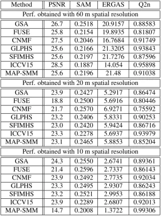
To assess the performance of the tested methods, as we do not have any ground truth information, we propose to compare their multi-sharpening outputs with those obtained using the ENVI im-plementation of GS [3]. To do so, we use the same performance cri-teria as in the previous section. However, these results must be care-fully interpreted. Indeed, a good performance index—i.e., a high PSNR, a low SAM, a low ERGAS or a high Q2n—only indicates that the fusion result obtained with a tested method is close to the one reached by GS. On the contrary, the fact that one performance index is “poor” only states that the reached performance is different from GS. At this stage, we are not able to decide whether the per-formance is “better” or “worse” than with GS. Table 2 summarizes the obtained results. One may see that, for each given spatial
resolu-4They are publicly available at https://scihub.copernicus.
Method PSNR SAM ERGAS Q2n Perf. obtained with 60 m spatial resolution GSA 26.7 0.2518 20.9157 0.88583 FUSE 25.8 0.2154 19.8935 0.81807 CNMF 27.5 0.2046 16.7684 0.91749 GLPHS 25.6 0.2166 21.3205 0.93843 SFIMHS 25.6 0.2197 21.7276 0.87596 ICCV15 28.5 0.1887 14.054 0.95898 MAP-SMM 25.6 0.2196 21.48 0.91038
Perf. obtained with 20 m spatial resolution GSA 23.9 0.2427 5.2917 0.86474 FUSE 18.8 0.2500 5.6916 0.80446 CNMF 21.7 0.2570 6.9271 0.75592 GLPHS 23.2 0.2406 5.8331 0.90253 SFIMHS 23.0 0.2420 5.9424 0.86716 ICCV15 23.3 0.2278 5.6937 0.93979 MAP-SMM 23.1 0.2465 5.8853 0.85204
Perf. obtained with 10 m spatial resolution GSA 24.3 0.2550 2.6741 0.89361 FUSE 21.4 0.2596 2.7337 0.86143 CNMF 23.9 0.2492 2.7735 0.92034 GLPHS 23.3 0.2495 2.9307 0.86243 SFIMHS 23.2 0.2521 2.9953 0.86188 ICCV15 23.9 0.2289 2.6807 0.92013 MAP-SMM 14.7 0.2008 1.3722 0.99306 Table 2. Reached performance wrt GS output on real data.
tion, all the tested methods (except MAP-SMM for 10 m of spatial resolution) provide a quite similar performance with respect to these indices. We thus can state that they globally provide a quite similar performance. However, when we visually look at the fused images, one might see some specific behaviors, as we now discuss.
Due to space constraints, we only show the performance reached for 60 m of spatial resolution. As the tested methods generate some datacubes which are not easy to draw in a compact way, we propose the following procedure. For each pixel, we average the amplitudes along the spectrum axis. We then derive an image that we draw ac-cording to the same scale. All these images are shown in Fig. 2. In particular, Fig. 2(a) represents the original 1830×1830×3 Sentinel-2 image that we aim to fuse with the 366 × 366 × 16 Sentinel-3 one plot in Fig. 2(b). Figures 2(c) to 2(i) show the obtained fused im-ages with the different tested methods. One may notice that most of them provide some artefacts. In particular, FUSE seems to provide the worst visual performance. Indeed, one notice some visible arte-facts providing a kind of texture. Moreover, it also provides some negative amplitudes which have no physical meaning. Then, please notice that the Sentinel-3 image seem to provide more spatial infor-mation that the Sentinel-2 one. This is probably due to the fact that, even if both images were taken the same day, they were not taken at the same time and that the considered Sentinel-2 data only con-tain 3 spectral samples. However, CNMF and GSA seem to provide a higher visual quality than the other methods. Both methods can also partially remove clouds from Sentinel-3 images. Then, both SFIMHS and MAP-SMM provide some similar images, with a vi-sually good spatial information. Lastly, ICCV’15 seems to stick to Sentinel-2 spatial information. However, this is not the case when the spatial resolution is 10 m—not shown for space consideration— where it provides the best visual information. Unfortunately, in the
absence of ground truth, it is hard to provide more information about these results, which is a perspective discussed in the next section.
5. CONCLUSION AND PERSPECTIVES
In this paper, we presented a first comparative study of Sentinel-2 and Sentinel-3 image fusion methods. As the ratio between high and low spatial resolutions increases, and for higher spatial resolution (10m), the fusion performance decreases. According to the consid-ered experiments, CNMF and ICCV’15 seem to be the more robust tested methods. In future work, we aim to propose a new method able to take into account all the bands of Sentinel-2 in order to pro-vide a new multi-spectral image with 10-m spatial resolution and Sentinel-3 spectral bands. Moreover, we aim to compare the above methods and our future work with in situ measurements. To that end, atmospheric correction [21] will be applied to Sentinel-2 and 3 data.
6. REFERENCES
[1] N. Yokoya, C. Grohnfeldt, and J. Chanussot, “Hyperspectral and multispectral data fusion: A comparative review of the re-cent literature,” IEEE Geosci. Remote Sens. Mag., vol. 5, no. 2, pp. 29–56, 2017.
[2] L. Loncan, L. B. De Almeida, J. M. Bioucas-Dias, X. Briot-tet, J. Chanussot, N. Dobigeon, S. Fabre, W. Liao, G. A. Lic-ciardi, M. Simoes, et al., “Hyperspectral pansharpening: A review,” IEEE Geosci. Remote Sens. Mag., vol. 3, no. 3, pp. 27–46, 2015.
[3] C. A. Laben and B. V. Brower, “Process for enhancing the spa-tial resolution of multispectral imagery using pan-sharpening,” 2000, US Patent 6,011,875.
[4] Q. Wei, N. Dobigeon, and J.-Y. Tourneret, “Fast fusion of multi-band images based on solving a sylvester equation,” IEEE Trans. Image Process., vol. 24, no. 11, pp. 4109–4121, 2015.
[5] P. Kwarteng and A. Chavez, “Extracting spectral contrast in landsat thematic mapper image data using selective principal component analysis,” Photogramm. Eng. Remote Sens, vol. 55, no. 1, pp. 339–348, 1989.
[6] N. Yokoya, T. Yairi, and A. Iwasaki, “Coupled nonnegative matrix factorization unmixing for hyperspectral and multispec-tral data fusion,” IEEE Trans. Geosci. Remote Sens., vol. 50, no. 2, pp. 528–537, 2011.
[7] S. Li, R. Dian, L. Fang, and J. M. Bioucas-Dias, “Fusing hy-perspectral and multispectral images via coupled sparse tensor factorization,” IEEE Trans. Image Process., vol. 27, no. 8, pp. 4118–4130, 2018.
[8] C. Dong, C. C. Loy, K. He, and X. Tang, “Image super-resolution using deep convolutional networks,” IEEE Trans. Pattern Anal. Mach. Intell., vol. 38, no. 2, pp. 295–307, 2015. [9] A. Korosov and D. Pozdnyakov, “Fusion of data from
Sentinel-2/MSI and Sentinel-3/OLCI,” in Living Planet Symposium, 2016, vol. 740, p. 405.
[10] Q. Wang and P. M. Atkinson, “Spatio-temporal fusion for daily sentinel-2 images,” Remote Sensing of Environment, vol. 204, pp. 31–42, 2018.
[11] F. Palsson, J. R. Sveinsson, and M. O. Ulfarsson, “Sentinel-2 image fusion using a deep residual network,” Remote Sensing, vol. 10, no. 8, pp. 1290, 2018.
(a) (b) (c)
(d) (e) (f)
(g) (h) (i)
Fig. 2. Fused Sentinel-2 (with 60 m spatial resolution) and Sentinel-3 images, with several methods: (a) original Sentinel-2 image, (b) original Sentinel-3 image, (c) GSA, (d) FUSE, (e) SFIMHS, (f) CNMF, (g) GLPHS, (h) ICCV’15, (i) MAP-SMM.
[12] M. Puigt, O. Bern´e, R. Guidara, Y. Deville, S. Hosseini, and C. Joblin, “Cross-validation of blindly separated interstellar dust spectra,” in Proc. ECMS’09, 2009, pp. 41–48.
[13] B. Aiazzi, S. Baronti, and M. Selva, “Improving component substitution pansharpening through multivariate regression of ms + pan data,” IEEE Trans. Geosci. Remote Sens., vol. 45, no. 10, pp. 3230–3239, 2007.
[14] B. Aiazzi, L. Alparone, S. Baronti, A. Garzelli, and M. Selva, “MTF-tailored multiscale fusion of high-resolution MS and pan imagery,” Photogrammetric Engineering & Remote Sens-ing, vol. 72, no. 5, pp. 591–596, 2006.
[15] J. Liu, “Smoothing filter-based intensity modulation: A spec-tral preserve image fusion technique for improving spatial de-tails,” International Journal of Remote Sensing, vol. 21, no. 18, pp. 3461–3472, 2000.
[16] C. Lanaras, E. Baltsavias, and K. Schindler, “Hyperspectral super-resolution by coupled spectral unmixing,” in Proc. IEEE ICCV’15, 2015, pp. 3586–3594.
[17] M. T. Eismann, Resolution enhancement of hyperspectral im-agery using maximum a posteriori estimation with a stochastic mixing model, Ph.D. thesis, University of Dayton, 2004. [18] R. F. Kokaly, R. N. Clark, G. A. Swayze, K. E. Livo, T. M.
Hoefen, N. C. Pearson, R. A. Wise, W. M. Benzel, H. A. Low-ers, R. L. Driscoll, et al., “USGS spectral library version 7,” Tech. Rep., US Geological Survey, 2017.
[19] Grupo de Inteligencia Computacional, UPV/EHU, “Hyper-spectral imagery synthesis (EIAs) toolbox,” http://www. ehu.es/ccwintco/index.php/Hyperspectral_ Imagery_Synthesis_tools_for_MATLAB.
[20] P. Jagalingam and A. V. Hegde, “A review of quality metrics for fused image,” Aquatic Procedia, vol. 4, pp. 133–142, 2015. [21] F. Steinmetz and D. Ramon, “Sentinel-2 MSI and sentinel-3 OLCI consistent ocean colour products using POLYMER,” in Proc. SPIE “Remote Sensing of the Open and Coastal Ocean and Inland Waters”, 2018, vol. 10778.