by
Brian Bennett Reinhold B.A. Brandeis University
(1976)
SUBMITTED IN PARTIAL FULFILLMENT OF THE REQUIREMENTS OF THE
DEGREE OF
DOCTOR OF PHILOSOPHY
at the
MASSACHUSETTS INSTITUTE OF TECHNOLOGY December, 1981
O
Brian Bennett ReinholdThe author hereby grants to M.I.T. permission to reproduce, and to distribute copies of this thesis document in whole or in rart.
Signature of Author
Department of Meteorology and Physical Oceanography December 31, 1981 Certified by Raymond T. Pierrehumbert Thesis Supervisor Accepted by Peter Stone Department Chairman SA SETTS iTUTE OF TECHNOLOGY
W~lT1q982
Liu LIBRARIESTable of Contents Background ... 1 1. Introduction ... 13 2. The Model ... 19 3. Model Scaling ... 26 4. Multiple Equilibria ... 34
5. Time Dependent Behavior ... 41
6. Model Synoptics ... 69
7. Synoptic-Planetary Scale Interactions ... 73
8. Summary ... 88
9. Estimates of Eddy Transports from Stability Theory ... 95
10. Synoptic-Scale Stabilization ... 109
11. Synoptic-Scale Transition Mechanism ... 128
12. Atmospheric Regimes ... 139
13. Conclusions ... 155
14. References ... 159
15. Description of Figures and Tables ... 162 Appendix I: How to Write a Highly Truncated Spectral Model 1.o Appendix II: Calculation of the Interaction Coefficients .5%
Appendix III: Obtaining the Mode 11 Equilibria I6A Appendix IV: Stability Calculation
al2.
by
Brian Bennett Reinhold
Submitted to the Department of Meteorology and Physical Oceanography on December 31, 1981 in partial fulfillment of the requirements for
the degree of Doctor of Philosophy in Meteorology ABSTRACT
We hypothesize that periods of quasi-stationary behavior in the large scales is integrally associated with an organized behavior of the
synoptic scales, thus the terminology "weather regimes". To investigate our hypothesis, we extend the model of Charney and Straus (1980) to
include an additional wave in the zonal direction which is highly baroclinically unstable and can interact directly with the externally
forced large-scale wave. We find that such a model aperiodically vacillates between two distinct weather regime states which are not located near
any of the stationary equilibria of the large-scale state. The state of the model flow may remain in either one of these two states for several synoptic periods. During each of the two regimes, the net transports by the transient disturbances are found to have consistent, zonally
inhomogeneous structure, the form of which depends upon the regime. This result implies that the transports appear as a net additional external forcing mechanism to the large-scale wave, accounting for the differences between the time mean regime state and the stationary equilibria.
Following the analysis proceedure of Frederiksen (1979), we show that the observed structure of these net transports can be accounted for by the spatial modulation of the baroclinically most unstable eigenmodes by the large-scale wave. We then consider only the tendency equations of the large-scale variables where the effects of the transients are
parameterized by solving the stability problem at each time step. We find that such a dynamical system possesses two absolutely stable "regime-equilibria" which are very close in phase space to the time mean states of the regimes appearing in the full model. We then demonstrate that the instantaneous component of the transients are also capable of transfering the state of the model flow from the attractor basin of one of the stable regime-equilibria to the attractor basin of the other. Our experiments thus indicate that the transients are important in determining the
qualitative behavior of both the instantaneous and time mean components of the large-scale flow in our system, and suggest that the very different
short range climates in the atmosphere can result from entirely internal processes.
Thesis Supervisor: Raymond T. Pierrehumbert Title: Professor of Meteorology
One of the most interesting, but poorly understood, phenomena in synoptic meteorology is the occurrence of
large-amplitude, planetary scale waves, which often persist for periods long compared to the passing of a transient
synoptic-scale wave. On a day to day basis, these phenomena appear as persistent, large-scale undulations or meanderings of the circumpolar westerly jet on middle and upper level tropospheric weather maps.
The impact of these events on regional weather can be quite significant, since migratory cyclones have a tendency to be "steered" by the upper level flow pattern. The maintenance of a quasi-stationary wave, or persistence in the upper level flow patterns, is then experienced at the surface as either
persistent or repetitive weather, depending upon ones relative position with respect to the tracks of the migratory cyclones. Surface regions sufficiently equatorward or poleward of the storm track would experience an extended period of dry warm or cold weather, respectively, while regions within the storm track may experience excessive precipitation or highly variable weather on a day to day basis, as a result of the passing disturbances.
remarkable persistence and obtains such large amplitude that the migratory cyclones are diverted far from their
climatologically determined paths for an anomalously extended period of time. These events are so strikingly prominent on
the daily weather maps that synoptic meteorologists have come to refer to the extreme example of a quasi-stationary wave as a "block" or an "omega block" since the undulation in the jet stream often resembles the shape of the Greek letter
2
.The persistence of a planetary-scale quasi-stationary wave and its associated pattern of migratory cyclones will be referred to as a "weather regime" in recognition of its
influence over a considerable fraction of the globe's surface weather. Blocking, from this viewpoint, is simply a special case of the more general weather regime phenomenon.
Weather regimes are perhaps more common than generally recognized, although some rather striking examples which have occurred over the North American sector during the period from
1976 to 1981 have substantially increased interest in this
phenomenon. At least two reasons may account for the lack of recognition of many regimes. One is that most regimes do not appear as striking as the relatively rare Eastern Atlantic block, for which the quasi-stationary component of the flow strongly dominates the fluctuating synoptic component of the flow. Another reason seems to be that unless the nature of
the weather induced by a given regime is sufficiently extreme to arouse publi-c interest, i.e., drought, heatwaves, excessive precipitation, etc., it will often exist unnoticed.
The concept of regimes has not always been so absent from the jargon of the meteorologist; in fact, at one time, the concept was actively pursued. In the early to mid nineteen forties several meteorologists, most notably Baur, Elliot, Krick, and Namias, studied a phenomenon which they referred to
as "weather-types" or "grosswetterlage". In the interests of extended-range forecasting, the studies catologued the shapes of the upper-level quasi- stationary waves and the associated tracks of cyclone events as well as the general flows of
surface warm and cold air. But for some reason, by the early nineteen fifties, the concept of weather-typing phased itself out of analytic meteorology and has since never gotten
re-established into the field.
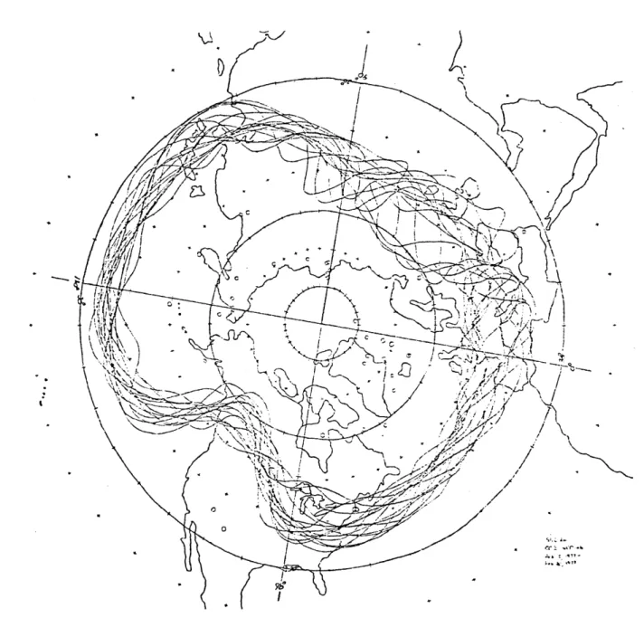
In order to clarify and establish more concretely the phenomenon of weather regimes, we now present a few examples of atmospheric cases. The occurrence of weather regimes (or quasi-stationary waves) is most easily demonstrated by
considering the limited-contour analyses of Sanders (personal communication). Since 1976, Professor Sanders at MIT has maintained what he has called Northern-Hemispheric Continuity Charts. These charts are generated by tracing and superposing
for periods of one week the daily 552 dam height contour of the OOZ 500 mb NMC final analysis (transmitted over NAFAX).
The quasi-stationary waves are defined by the envelope or "eyeball average" of the daily contours. Regions over which the flow is steady will generally be marked by a narrow,
fairly constant meridional width envelope while regions where the flow is unsteady will generally be marked by a wide and bulging envelope. From the presently accumulated 4.5 year
sample (which excludes the months June through August) there are several cases which can serve to illustrate the occurrence of atmospheric weather regimes.
The first example to be considered is the 18 day period from January 26, 1980 to February 15, 1980, shown in Figure A. This was the year that brought record breaking drought to the Olympic Winter Games in the Northeastern United States and record snowfalls to the Southeast States. The most prominent steady features which appear on the map are the large-scale trough which occurs just downstream of the highly disorganized flow over the Eastern Pacific and Western North America, and the near zonal flow from Central Asia to the mid-Pacific. In addition, there appears to be a somewhat more disorganized, smaller scale, ridge-trough-ridge pattern over Europe and Western Asia. However, it is not possible to ascertain from the analysis whether the "disorganization" is real or an artifact of the lack of two- dimensional information. (For
example, if the height gradients of the quasi- stationary pattern over Europe happen to be markedly weaker than other regions about the globe, a given synoptic-scale transient disturbance will produce a higher amplitude "wiggle" in that
location, introducing a spuriously erratic appearance to the otherwise steady regime). Over the Eastern Pacific and
Western North America, on the other hand, the erratic behavior is much more evidently a consequence of unsteady flow, for the
fluctuations are primarily larger scale.
The Eastern North America-Atlantic trough case is an excellent example of the dramatic influence a regime can have upon the behavior of the transient disturbances. The
asterisks, eight of which are concentrated in the Western Atlantic, correspond to the occurrence of surface "bombs"
(explosively intensifying cyclones) as defined by Sanders and Gyakum (1980). According to Sanders and Gyakum, this
frequency of bombs is excessive, suggesting the presence of a regionally highly active baroclinic zone. Many of these bombs
initiated in the Gulf States (a process which, combined with the southward extent of the cold trough, brought the Southeast
States anomalous snowfall amounts) and exploded out over the Gulf Stream, but the deepening cyclones repetitively were
"steered" too far to the east to bring precipitation to the dessicating, anomalously cold, Northeast States. Though we
large-scale configuration, we do not mean to imply that such is the case here. (Indeed, we intend to show that it is
equally likely that the repetitive bomb events were necessary to maintain the large-scale pattern).
The second example, plotted in Figure B, is the period from February 5, 1977 to February 20, 1977, which is the last
16 days of the now infamous winter regime of 1976-1977.
Outside of the very prominent ridge-trough pattern over North America, the flows are basically zonal across Europe followed
by a low amplitude Central Asian ridge and Western Pacific
trough. A significant difference between this 16 day period and the February, 1980 case in Figure A is that the flow
appears quite steady everywhere about the globe.
The feature of interest, however, is the high amplitude ridge-trough pattern over North America. This pattern was established well before the first day included in the figure,
being recognizable as early as the previous October, making this particular regime the longest lasting regime of the data set. The weather associated with this regime had economically disastrous consequences across much of the United States: the west coast suffered severe drought and anomalous warmth, while the east coast, especially the Central East States, was
One of the most spectacular features of the 1976-1977 ridge-trough regime was its sudden collapse. Figure C is a
plot of the 15 day period from February 22, 1977 to March 8,
1977, which directly follows the period shown in Fig. B, save
February 21. The ridge-trough pattern, which had persisted for longer than four months, was completely obliterated in less than two days. In contrast, the rest of the globe, except for Europe, remained essentially unchanged.
The third example, shown in Figure D, is another high amplitude ridge- trough regime over North America, similar to
the 1976-1977 case. This plot encompasses the 16 day period from December 31, 1980 to January 15, 1981 (which marked the end of the 4.5 year data set). The 1981 regime, similar to the 16 day period selected in the 1977 case, is accompanied by steady behavior about the globe, again with a low amplitude mid-Asian ridge and Western Pacific trough. However, the flow
over the Eastern Atlantic and Europe is markedly different. In the 1981 case, a large-amplitude ridge-trough pattern
extends from the Central Atlantic across Europe, in contrast to the zonal flow observed in the 1977 case (Fig. B).
The weather associated with the 1981 North American ridge-trough regime is subtly different from the 1977 case. First, the regime did not become established until the last days of December 1980, and persisted only about 18 days or so.
Second, the feature has a somewhat greater amplitude with a trough axis further east than the 1977 case. The subtle eastward shift has brought polar blasts down on New England instead of the Central East States. These outbreaks result in substantially colder weather in New England and the East Coast States since the cold air is not modified by the eastward
travel across the Appalacians as in 1977. In addition, warmer temperatures have crept further eastward across the Great
Plain States.
The paths taken by cyclones during this regime were remarkably repetitive. Weak Alberta cyclones traveled southeastward into the Great Lakes Regions and turned
northeastward, perhaps associated with weak coastal secondary cyclogenesis. As the primary or secondary storm moved
northeastward, it rapidly intensified, too far to the north and east to bring substantial precipitation amounts west of Newfoundland, but not sufficiently far north and east for the Northeast States to avoid the cold arctic blasts on the
leeward sides of the intensifying storms.
The last two cases, shown in Figures E and F, are
examples of a regime which has not been too common during the winters since 1976; ridging in the Eastern Pacific and
troughing on the West Coast followed by a disorganized attempt at East-coast ridging. This pattern, in a gross sense, is the
reverse of the 1976-1977 and 1981 cases. Figures E and F consist of the 20 day period from March 14, 1977 to April 2,
1977 and the eleven day period from March 26, 1979 to April 5, 1979. The flows in both examples have considerable synoptic signal over North America and, in the 1977 case, part of Western Asia. The remainder of the global flow patterns (except over the Eastern Pacific) are, on the other hand, considerably different in the two cases. The weather
associated with these North American regimes seems to have two possibilities for the East Coast. The tendency for East-Coast ridging brings anomalous warmth, but the highly variable
synoptic waves often develop into cutoff. circulations which linger painfully over the Western Atlantic, bringing extended periods of drizzle, rain, cloudiness, and otherwise general misery, to the Northeast Coast. In the March 26-April 5 case of 1979, it rained 8 out of the 11 days at Logan airport in Boston, Mass., while in the March 14- April 2, 1977 case, a drizzly, rainy period was followed by a heat wave.
There are several other examples of persistent
atmospheric states which have not been displayed. Two of noterity were the ridge-trough regimes over North America during the 1977-1978 and 1978-1979 winters, both of which persisted on the order of 30 days. Each brought heavy precipitation amounts to the eastern United States but a subtle shift in the position of the large- scale trough
between the two cases resulted in heavy snows one year on the East Coast followed by heavy rains in the succeeding year. Another event of note was the intense heat wave of the 1980 summer. Though the summer months were not analyzed, one can be reasonably confident that the heatwave is undoubtedly associated with an anomalous weather regime.
SUMMARY
The limited number of examples above are presented primarily to familiarize the reader with the phenomenon of interest and enable him or her to visualze this otherwise difficult-to-describe feature. Though there is insufficient data to provide conclusive evidence about the behavior and properties of the weather regimes, there are a few statistics of note which can be surmised from this limited sample. First and foremost, there is an extreme diversity in the observed regime persistence, with (subjectively determined) durations ranging from as short as 11 days to as long as 130 days, with no clear evidence of a preferred time scale. Second, regimes appear to be rather strongly localized. This property was evident in the February 1980 case (Figure A), where one sector of the globe varied erratically while other sectors remained essentially unchanged, and in the transition of the 1976-1977 regime (Figures B and C), where the North American sector underwent a radical transition while the ridge-trough over
Asia and the Western Pacific persisted with no change. Third, a few regimes were noted to establish and or collapse at rates approaching a synoptic time scale.
In spite of the presentation of some fairly well defined "textbook" cases, it remains an extremely difficult task to precisely quantify the weather regime (a problem discussed by Dole, 1982). For this reason it is necessary to explicitely point out the distinction between the weather regime and the
"stationary" and "transient" wave decomposition frequently used in general circulation studies, with which it may be confused. The stationary wave is computed as the residual non-zonal component of the atmospheric flow field averaged over some (arbitrarily) chosen time period, i.e., a month, season, year, etc. Though a regime may persist for as long as a season, such instances appear to be exceptional, and it is generally unlikely that the stationary wave decomposition will adequately represent the weather regime phenomenon. Since the majority of observational studies consider several months,
seasons, or even years in their analyses to generate the
stationary and transient components, we may reasonably assume that several regimes, fractions of regimes, as well as periods of "unsteady" flow, are included in the data, and thus a
single regime will be partitioned in an unknown manner between the stationary and transient components. It is evident from the qualitative description provided in this section and the
techniques used to compute the stationary and transient waves, that the three features represent distinctly different
entities. The stationary waves, in this case, may simply represent an "unoccupied average", e.g., the weighted average of the various regime states.
The purpose of this dissertation is to investigate the weather regime phenomenon. Based on what we have described in this section, a potentially very important aspect of the
regimes so far neglected in theoretical studies is the influence of the organized behavior of the synoptic-scale
disturbances. The investigation of the role of the transients and their feedbacks upon the planetary scales during periods of weather regimes as well as periods of regime transition is the primary new contribution of this work.
1. INTRODUCTION
The occasional persistence of certain large-amplitude planetary-scale atmospheric features and their influence upon the behavior of the transient synoptic-scale disturbances has long been noted by forecasters and synoptic meteorologists. Among such persistent events, the group of phenomena known as
blocking is perhaps the most striking. Although blocking has been the subject of much research, the dynamical processes which establish and maintain these quasi-stationary features and couple them to the baroclinic disturbances are not yet well understood.
A promising approach toward explaining blocking is
provided by the concept of multiple flow equilibria introduced
by Charney and DeVore(1979). The multiple flow equilbrium results suggest that the atmospheric flow system in the
presence of zonally inhomogeneous external forcing mechanisms (e.g., topography, land-sea contrasts, heat sources and sinks, etc.) can possess not one, but several equilibrium flow
configurations. The hypothesis, as stated by Charney and DeVore, is that the general behavior of the atmosphere can be understood as a flow which is driven by smaller scale
instabilities from one quasi-stable equilibrium point to another. In this theory, the particular event of blocking occurs when the atmospheric trajectory approaches a
quasi-stable equilibrium solution which possesses both a high wave amplitude and low zonal index configuration.
One of the more important assumptions of the multiple flow equilibria theory (MFET) is that some of the equilibrium flow configurations in the atmosphere are quasi-stable in the sense that a solution starting from an initial condition not too.far from the equilibrium point remains close to that point for a long period of time. However, we are interested in the time dependent behavior of the solution after long periods of time, far from the initialization, i.e. once the solution has settled down into its attractor. It is not always clear that the equilibria form part of the attractor, unless they are absolutely stable. If the equilibria are stable, we know that once the trajectory enters a finite region about the
equilibria, it will remain confined to that region and approach the equilibrium state. In that case, the time
dependent problem becomes trivial. However, if the equilibria are all unstable, there are no mathematical grounds upon which we can make the assumption that the equilbria and the time dependent behavior are related.
Several authors have studied the stability properties of equilibrium states in various highly simplified models. Most of these studies considered barotropic atmospheres. The
weakly unstable to all perturbations (see Charney and DeVore(1979) and Charney et. al. (1981)). These
observations provided the primary motivation for explaining the quasi-stationary disturbances of the atmosphere as
manifestations of these equilibria. The analysis of the baroclinic equilibria, on the other hand, results in
substantially different conclusions. For realistically large values of the driving, Charney and Straus (1980) and Roads
(1980a,1980b) found that the baroclinic equilibria were highly unstable to smaller scale perturbations. However, it was
generally assumed that the effects of the synoptic scale instabilities were minimal and thus it was concluded that
"realizable" equilibria, i.e. those which would be part of the time dependent attractor, were solutions which were found to be stable or weakly unstable to perturbations restricted to the scale of the equilibria. These assumptions, however, have not been validated and clearly require further investigation.
We do know that the real atmosphere is highly
baroclinically unstable to perturbations on the synoptic
scale, in the sense that we frequently observe rapidly growing disturbances on such a scale. a priori, it does not seem
possible to predict the manner in which the vigorous
synoptic-scale baroclinic disturbances of the atmosphere will interact with the theoretical stationary solutions. It is entirely possible that the instabilities may destroy the
equilibria, as they will most-likely extract energy from the large scale. Indeed, it is not clear whether the stability of the analytically- derived stationary solution with respect to perturbations restricted to the scale of those solutions will have any relevance to the phase space behavior of a system including the synoptic scales. Thus we must study the manner
in which the highly active synoptic-scale waves interact with the externally forced stationary waves.
Theoretical and observational studies indicate that the interactions may be significant for both the synoptic and
large scales. A modeling study by Frederiksen (1979)
demonstrated that the presence of a prescribed planetary-scale wave modulated the baroclinic disturbances in such a manner that the spatial configuration of the net transports by the instabilities had distinct maxima relative to the phase of the large scale wave. In a similar modeling study, Niehaus (1980) showed that a prescribed basic state with wavy structure could also account for the occurrence of storm tracks in terms of certain regions of the basic state wave which were more active baroclinically. In both cases, it is apparent that the
presence of a large- scale wave acts in some manner to organize the transients. On the other hand, Gall et. al.
(1979), using a general circulation model, demonstrated that
the small-scale transient disturbances are capable of forcing planetary scale circulations without the presence of any
zonally inhomogeneous ror:ing or initial planetary scale perturbations. In addition, Sanders and Gyakum (1980) in
their observational analvsis have noted the sudden
amplification of plane-ar-y scale ridges just downstream of a region in which severa. successive explosively deepening
cyclones have occurred. :n these studies, it is apparent that the synoptic scales are capable of forcing and altering the large scales.
The combination of tzea organization of the transients by the planetary scale, and ihe forcing of the planetary scale by the organized transients suggests a potentially significant feedback process. It is reasonable to expect that these interactions could esta.zlish some type of balance. This possibility provides a meChanism through which the highly unstable externally forzed planetary scale wave considered in
the MFET can equilibrate with its own instabilities. The
basic hypothesis in this zaper is that exactly such a feedback process is responsible f=- the occurrence of quasi-stationary behavior in the atmosphoere.
Our hypothesis imcp.es that quasi-stationary behavior in the planetary scales is .t.egrally associated with an
organized behavior of t-ne synoptic- scale events. In
recognition of the fact ::st the synoptic scales are generally responsible for what is c:nsidered "weather", these
quasi-stationary periods will be referred to as weather
regimes. The event of blocking, then, which is an unusually steady, high amplitude quasi-steady state, is simply a subset of the more general weather regime phenomenon.
We shall investigate the weather regime phenomenon in the simplest possible model that has the necessary physics to
incorporate the feedback process alluded to above. This will be accomplished by extending the model of Charney and Straus
to include an additional wave in the zonal direction in such a manner that it can directly interact with the externally
forced planetary scale wave. The first aspect of the analysis will be to consider the properties and characteristics of the model theoretical equilibria. We then examine the
time-dependent behavior of the model and investigate the
appearance of regime-type phenomena. We can then consider the qualitative properties of the regimes as a function of the parameters and their relation to the corresponding
theoretically calculated equilibria. The final aspect of the theoretical analysis will be to consider the behavior of the synoptic scales and their roles during both persistent periods and times of transition. In conclusion we will attempt to ascertain in what manner the theory developed in this paper can help us to understand the complex weather regime behavior in the atmosphere.
2. THE MODEL
Our model is essentially the same as the highly truncated two-layer spectral channel model of Charney and Straus (1980). The important difference between the two models is that we retain two waves in the zonal direction so we can represent a baroclinically unstable synoptic scale wave that interacts directly with the large scale wave. As in Charney and Straus, we will use the notation devised by Lorenz (1960b) where
LV= .( * + 'P ) is the mean streamfunction, t = ( ',- 94 ) is the mean shear streamfunction, G + G3)( ) is the mean
potential temperature, G = e , - &,) is the static
stability, which is assumed constant, and , = is the velocity potential. The subscripts 1 and 3 refer to the middle of the upper and lower layers, respectively. The
system of equations becomes:
afi/7t
+ J(T
, z V) + J( -2-, V'2- ) + Ly/n x -. 5 J( T,ffi/H) + .5 J('2,ffi./H) + k''V2-'-_) + J( q , q2C ) + J( C, V-) +f387'/Qx
- f V= +.5 J( ,fh/H) - .5 J( t,f'a/H) - k'' -k;G/,t
+ J( G'X- G\7)=
h''(-8)
(2.1)where the Jacobian J(A,B) is defined as
QA/ax J)B/cy-;B/hx )A/cy, f is the coriolis parameter 2asing(, where is some specified latitude and.Q is the angular velocity of the earth, /2 is the gradient of f, 1/a,(Jf/Ad),
where as is the radius of the earth, VI)Lis the horizontal
divergence given by the continuity equation 979=-ow/Ap where w
is the pressure velocity, k'' is the Ekman damping coefficient at the surface, k '' is the Ekman damping coefficient between
the layers, H is the thickness of each layer, 6iis the topographic height, where hi0/H
<<
1, h is the Newtioniancooling coefficient, and
e&
is a prescribed radiativeequilibrium temperature field. The system of equations is closed by the thermal wind relation
2-r= -(c~b*/2f)V 9
(2.2)
where cgis the heat capacity of air at constant pressure, and b equals (p, /p. ) -(p, /p. ) where p, and p. are the pressure levels at the center of the two layers (400 and 800 mb,
respectively), p. is the surface pressure, 1000 mb., and K is the ratio R/c,=2/7, where R is the gas constant. This form of
the thermal wind relation for a two layer model is derived by Young (1966). For details of the model, see Appendix I.
Following Lorenz (1960a), we will maximally simplify the two layer quasi-geostrophic system by expanding the dependent variables in orthonormal eigenfunctions of the Laplace
operator 72and retaining the fewest number of modes possible that still possess the necessary physics to simulate the
hypothesis, the model must contain the interaction between an externally forced planetary scale wave and a baroclinically unstable synoptic scale wave. We must choose our truncation such that this minimum requirement is met.
The decomposition of the equations into spectral form is given by Lorenz (1962, 1963), Young (1966), Yau (1977,1980), Charney and DeVore (1979), and Charney and Straus (1980) and will not be repeated in detail here. In essence, we write the equations in dimensionless form and expand the dependent
variables in terms of the orthonormal eigenfunctions F;. The expansions and the relations between the nondimensional(RHS) and dimensional(LHS) forms of the parameters and the dependent variables (where the nondimensional dependent variables are denoted by subscripts) are given by:
LV Fj=-a F,.
=L2 f Y WF 7=f f w;F.- k' '=fk
't
=L
.''F.e
F;f
=ALa f GF
k' ''=fk'
G=ALe f G;F to=t/f h''=fh
= H 7_-iF1,
P
=(L/a. )cot96 G =AL fG',x. =xL yo=yL = G (Thermal wind)
(2.3)
where L is some horizontal scale factor, A=-(2f/cgb" ), and to,
x., and y. are the dimensional forms of the time and eastward
and northward coordinates, respectively. The spectral form of the equations is obtained by substituting the above expansions
into the original equations. We obtain: + b
/a.h-3~c
[ (a -ak )( +9 +.,Ja I+ w + h( G ;)T- ( a ( + )+ -ti(G -
)
+ )]/a. b /a k (9 - G;) 9;=IF-c~ 1,~~
~
~
,)
- -h (9-)
- (1 -Gi) I/ aPk
I
3
.
+ bG/a
- w;/al + kM'. - (k + 2k' G; (2.4)where cY,; =L2 /27t F; J(F ,F' )dx dy are the interaction
coefficients, and b , = L/27t
fF
F, aF, /.x dx dy. This system can be further simplified by eliminating w;between the twoequations.
Our model, like that of Charney and Straus, is a channel model with zonal walls at nondimensional y=O and y=7tand is subject to the boundary conditions of no flow through the wall and no net torque or momentum drag on the wall. The
rectangular geometry and these boundary conditions determine the final form of the allowable orthonormal eigenfunctions F;.
We will choose to truncate the model at two waves in x and two waves in y. This is the fewest number of components possible that provides a planetary scale and a synoptic scale and a nonzero wave-wave interaction coefficient. This
wave-wave interaction coefficient is the main new feature of this model and is the dynamic mechanism through which the planetary scale and the synoptic scale are directly coupled.
We will label these eigenfunctions as Fiwhere = 1,2,3,... ,lO. They are: Mode 11 Mode 21 F, =T2 cos(y) F ,=2 cos(2y) F = 2 sin(y)cos(nx) F5= 2 sin(2y)cos(nx) F = 2 sin(y)sin(nx) F = 2 sin(2y)sin(nx) Mode 12 Mode 22 F = 2 sin(y)cos(2nx) F,= 2 sin(2y)cos(2nx) F = 2 sin(y)sin(2nx) F = 2 sin(2y)sin(2nx) (2.5)
where n is one half the ratio of the meridional wavelength to the zonal wavelength and is related to the global wavenumber m
by m=nascos /L. In addition, we have classified each set of eigenfunctions into "modes" which represent the scale of the particular two dimensional wave and zonal flow (both the Mode 11 and Mode 21 variables contain eigenfunctions which have only zonal structure, i.e. F, and F, ). For example, Mode 12 corresponds to one wave in y and two waves in x,
1W, and Y . In this manner we can categorize what scales of
motion influence a given variable. From the form of the equations, we note that only topography and the nonlinear
advective terms provide coupling mechanisms between the modes. The remaining linear terms are effective only within a given mode.
ordinary differential equations for the amplitude coefficients of the ten eigenfunctions of the streamfunction
Y
and the potential temperature G . Before the equations can be written down, we must decide upon the form of the heatingG
and the topography Ifi.. To best-simulate the equator to pole differential heating, the model will be driven byapplying only a zonally symmetric south to north temperature difference, thus all components of are zero except 6. The nondimensional heating profile is then given by
6(y)=2
Gecosy, which is a fairly good first approximation
of the earth's equator to pole radiative equilibrium
temperature field. Topography, then, will provide the only zonally inhomogeneous forcing in the model. For consistency with our hypothesis, we require that the flow be forced at the
largest possible scale, which is designated by the
eigenfunctions F and F,. For simplicity, only the amplitude of the F. topographic component will be chosen different from zero. The final model equations become:
(See following pages) (2.6)
where the non-zero interaction coefficients (the calculation of the interaction coefficients is given in Appendix II) are:
-842 n/157L = c, /5 = c, /4 = c3/1O =c,/8
=
c,/16(2.7)
I. 2. 2
and the eigennumbers a, ,a , a 3
a, = 1 a =(n +1) a
=(n +1)
a= 4 a =(4n Z+1) a a, =(4n +1) S? a7 ,..., a are:as =(n +4)
a
=n 1+4)
= (4n (++4) =(4n +4) (2.8)From the form of the equations we note that there are certain independent subsystems. For example, if all the variables except the Mode 11 variables are set to zero, they will remain zero. The remaining tendency equations for the Mode 11 variables then form an independent subsystem. Other
independent subsystems are:
i.e., Modes 11 and 22.
3. MODEL SCALING
One of the most important aspects of any model study is the degree to which the model under consideration simulates the atmosphere. Even this particular very simple highly
truncated model contains parameters representing the magnitude of various physical effects, such as Ekman friction. Though we can always set these parameters to values we consider appropriate to the atmosphere, this does not guarantee that the model will behave in a manner that we would consider as realistic. The severe truncation and lack of smaller scales undoubtedly enhances the sensitivity of the few remaining scales of motion to the parameters. In fact, it may not be possible to simultaneously have both the dimensional values of all the parameters and the qualitative aspects of the time dependent flow "earthlike". It is reasonable to assume that at least some of the parameters will have to be adjusted to
compensate for the effect of spatial scales and physical processes left out of the model.
The relation between the dimensional and nondimensional variables and external parameters is given by (2.3). All we
need do then, is to select appropriate values for L, H, f, and the dissipative time scales and all the nondimensional
parameters are determined. However, of these scale factors and time scales, only f is known precisely. There are a range
of acceptable values for L, H, and the dissipative time scales which lead to a large range of nondimensional parameters for
our model which are arguably earthlike. The problem, however, is not so much the scaling, but the sensitivity of the model to the external parameters. For example, estimates of the atmospheric dissipative time scale easily vary by a factor of three; however, in our model, a factor of three difference in the nondimensional parameter k results in qualitatively very different flows. We shall therefore consider a range of nondimensional parameters and scale factors which arguably correspond to atmospheric values, and then subjectively
determine whether or not the qualitative behavior of the model flow is atmospheric. Each category of parameters will be
considered individually.
1). The dissipative parameters
Appropriate values for the atmospheric dissipative time scales (k'') and (h'') are generally ascertained to range from about 6 to 20 days. If we select f to be 10 /s, its
approximate value at 45 north, then the corresponding
nondimensional parameters k and h range from .02 to .005. The internal dissipative time scale, (k'') , which is not well known (but should be very long), will be taken to be about an order of magnitude longer, which gives a nondimensional range of values for k' of .002 to .0005.
2). The beta effect.
Beta is scaled by Lcot//a~where a0is the radius of the
earth, about 6400 km. An approximate range for L will be taken to be 1200 to 2000 km., or a channel widthiL=4000 to
7000 km., which gives a nondimensional beta of .18 to .33 at 45"N. However, a change of only 5 degrees latitude in where
we choose to center our channel (which also changes f slightly), say from 45 to 50 N with L=1600 km., changes
nondimensional beta from .25 to .21. Consequently, even for fixed L there is considerable flexibility in our selection of beta.
3). The temperature parameters.
The temperature scales depend upon the parameter A which is determined by the thermal wind relation (2.2). If we
choose our model top to be at 200 mb, and the surface to be at
1000 mb., A=1.1886X10 s*K/cm3 (see Young, 1966), which for our
previous range of L, gives a range in the quantity AL f of 170 to 475. Typical values of the north south radiative
equilibrium temperature difference are given by 70 to 200 * K (Stone, personal communication). In our model, since the heating is given by e(y)=2 G*ALtf cosy, appropriate nondimensional values of G, then range from .05 to .25.
The static stability measures the temperature difference between the middle layer and the upper or lower layer, which in our model is separated by 200 mb. Appropriate values for the lapse rate of potential temperature over the depth of the atmosphere range from perhaps as low as 50K/200 mb to 150K/200
mb. For the US standard atmosphere, the lapse rate is approximately 11"K/200 mb. These values correspond to a nondimensional range of G' from about .02 to .06 for the previously mentioned range of L.
4) Topography
The topography is scaled by the thickness H of each model layer. Since we have chosen the model top to be at 200 mb., the thickness of each layer is about 400 mb. which
corresponds to an H of about 4 to 5 km. The dimensional mountain height is then given by 'i=2Hn sinycosnx. The
nondimensional value of fi is then restricted by the condition that h,<<.5.
5) Wavenumber
The parameter n corresponds to the global wavenumber m through the relation m=na.cos
#/L.
The selection of n then determines the scale of the longest wave in our model. To be consistent with our hypothesis, we must select n such that thelargest scale in our model corresponds to a planetary scale disturbance, i.e., m<5, but more importantly, n must be chosen such that the 2n wave (Mode 12) is more unstable
baroclinically than the n (Mode 11) wave. To meet both of these criteria, we find that n generally must be less than
1.5.
In summary, "arguably" earthlike ranges for our 8 nondimensional parameters are then given by:
k=.005 to .02, k'=.0005 to .002,p =.15 to .35,
2h <.35, h=.005 to .02,
G=.02
to .06,G
=.05 to .25, and n<l.5.(3.1)
Though we cannot justify completely independent variation of certain parameters, we see that there is still considerable flexibility in the range of nondimensional parameters that correspond to earthlike conditions.
However, time dependent calculations with the above nondimensional parameters indicate that the qualitative behavior of the flow does not become "earthlike" until we
substantially increase the dissipative parameters and slightly increase the static stability. With the values of the
dissipative parameters as they stand, the model has a tendency to develop absurd easterly surface flows (>40 m/s) with an associated near zero zonal flow aloft, a configuration far
from an earthlike situation. The reason for this behavior is not entirely clear, but the fact that the problem can be
eliminated by sufficiently increasing the nondimensional
dissipative parameters suggests that excessive dissipation is necessary to compensate for the lack of eddy damping that would normally be present in an untruncated model. (The lack
of eddy damping in highly truncated models is also discussed
by Young (1966)). We have found that increasing the
dissipative parameters to values where k and h are greater than .03 is generally sufficient to limit the surface
easterlies to reasonable speeds for most ranges of the other parameters.
With the values of the static stability as they stand the time integrations lead to flows in which the small scale
circulations are too vigorous, i.e., all the energy is
contained in these scales. This problem is directly related to ascertaining the scale height H, or the thickness of each layer of the model. Our selection of 200 mb. as the model top has inadvertently given us an H of 4 to 5 km. However, from the dispersion relation for baroclinic instability in a two layer model (see Pedlosky(1979)) it is found that in order to best simulate the baroclinic dispersion relation of the continuous atmosphere, H should be 7 to 8 km., the typical scale height of baroclinically unstable modes in the
the model atmosphere then appears to extend into the stratosphere. The problem is that we cannot relate the pressure levels and corresponding heights of the observed atmosphere directly to the two layer approximation and simultaneously simulate the baroclinic processes in the continuous atmosphere. Consequently, since it is more
important to simulate the physical processes of the continuous atmosphere, we "stretch" the pressure height relationship in the sense that the 600 mb. level centers at 7 to 8 km.
instead of 4 to 5 km. as observed. The stretching of the scale height also demands that the nondimensional values of the static stability and mountain heights must also be
stretched. The dimensional static stability and mountain heights that correspond to these stretched nondimensional values then appear unrealistically large, but if they are viewed relative to the pressure levels instead of the scale heights, they become much more realistic. With these
considerations, the dimensional static stability parameter
G
ranges from about .08 to .20.With these alterations, the following ranges of
nondimensional parameters will be considered as "atmospheric" and appropriate for experiments:
k=.03-.06 k'=.001-.02
(
=.15-.35diZ <.35
h=.03-.06
G'
=.09-.20
,=.05-.25 n<1.5. (3.2)
As mentioned above, it is not entirely correct to select any arbitrary combination of the 8 parameters. Thus we have
considered a range of parameters that result in flows which, qualitatively, are earthlike, primarily to de-emphasize the practice of quantitatively associating a given parameter set with a specific set of external conditions on the earth. However, if we fix L=1600 km., we can narrow our choice of
parameters somewhat, though we may wish to vary parameters such as B , , and n beyond values which we consider as
earthlike for academic purposes. In any case, with L fixed as above, acceptable ranges for the nondimensional parameters dependent upon L become:
=.20 to .27
G;0=.09 to .18
e=.
0 5to .25
n<1.5
4. MULTIPLE EQUILIBRIA
There already have been a host of studies concerned with the multiple flow equilibrium problem, therefore we will not consider the properties of the equilibria in any great detail. We are primarily interested in obtaining the model equilibria
to study their relation to the time dependent behavior of the model when the effects of synoptic-scale instabilties are
included.
To obtain the equilibria we could set the tendency terms to zero and solve the twenty simultaneous nonlinear equations for the twenty variables. This would be an arduous if not impossible task. However, obtaining all the equilibria for the twenty variable system is most likely unnecessary. As we have pointed out in the Introduction, any equilibrium state is
highly baroclinically unstable to synoptic-scale perturbations
(this claim will be explicitly demonstrated shortly through the examination of the stability problem). Though there are undoubtedly model equilibrium solutions with synoptic-scale components, rapidly growing instabilities at the synoptic scale are likely to destroy any degree of organization of the time mean state at this scale. This suggests that we
concentrate our efforts upon obtaining only the large-scale equilibria. In our model, the planetary scale corresponds to the directly externally forced Mode 11 variables, which form
an independent subsystem. Thus the equilibria for the Mode 11 prognostic equations are also solutions to the entire twenty variable model.
The implication that only the Mode 11 equilibria are important to the time-dependent behavior of the model is an assumption which can only be truly justified in hindsight. If
the synoptic-scale components of the equilibria were
important, we would expect to see some signal from them in the time mean, but as will be seen shortly, the only non-zero
components in the time-average state of the model flow are the Mode 11 variables.
The Mode 11 system of equations, from which our
equilibria will be calculated, is identical to the system from which Charney and Straus obtained their equilibria. To solve the system we reduced the 6 equations in 6 variables to one algebraic equation in 9% which is solved numerically by a one dimensional binomial chop, (for details, see Appendix III). Consequently, we can always obtain all the roots for any set of external parameters, limited only by the resolution of the computer. The Mode 11 equations are:
0= c,% Z2 - (+ 1-k ( Y, - G,)
0= c, n ( e++ 33G )+/ n+' -k(n +l)(-G)
O=-c,
n
(++ G2-n -n+1(W-&)c3( -)O= c, ( 4- 4,Ge ) +c, c;, ii, (P-9e )+h(
91
- 9,)J+kg -c, (k+2k ' )oc;G,
O=-c,[ (1- c n? )4 -(l+ %n4 ) 1+flnD, -hG +k c; (n +1), -(ni+1)
g
(k+2k' )G
O= c,[ (1- G n7)G,+, -(1+ c(n? )41 e, If G;ne.-h, +k ag (n'+1)41
- (n + 1) 06 (k+2k')13+ ci
,(4.1)
One solution, which can be obtained immediately by
setting all the wave variables equal to zero, is the purely
zonal equilbrium state referred to as the Hadley Solution by
Lorenz (1962, 1963).
From the 41 tendency equation we see
4= Gwhich implies that there is no surf ace f
low and thus no
interaction with topography. From the etendency equation we
obtain
G,%
h 0% /(2k' G70 + h).All the remaining equilibria have nonzero wave components and
can only be obtained numerically.
It is not possible to investigate the complete behavior
of the wavy equilibria as a function of the eight parameters,
but some qualitative aspects of the solutions can be
others fixed. There are two qualitative aspects of the equilibiria that are of interest to this study. First, we find that the phase and amplitude of the equilibria are very sensitive to small changes in the external parameters,
especially k, ,i l3 , Gand n (for example, see Figure 1). As mentioned previously, the extreme sensitivity of the
equilibria is probably an artifact of the severe truncation. Second, the wavy equilibria occur in pairs; thus the total number of solutions, including the Hadley state, is either one, three or five. At least one of these pairs of wavy equilibria consist of a trough near the mountain ridge while the other solution consists of a ridge (though by no means related by a simple 180 degree phase shift), suggesting the super and subresonant locking phenomena discussed by Charney and DeVore (1979) and Roads (1980a, 1980b).
One property of the equilibria that is of interest to this study is the stability of the equilibria to the various modes. This property can be ascertained in the standard manner by linearizing the model equations about the various equilibrium states and solving an eigenvalue problem for the growth rates 1. The form of the equations is such that the eigenmodes separate into either pure Mode 11, Mode 22, and coupled Mode 21 and Mode 12 structure (the perturbation
matrices are given in Appendix IV). The eigenvalues '6 of the pure Mode 11 and Mode 22 eigenmodes then determine the
stability of the equilibria to Mode 11 and Mode 22
perturbations respectively. To determine the stability of the equilibria to Mode 12 and Mode 21 disturbances we must
consider the detailed structure of the unstable coupled eigenmodes to ascertain which perturbation scale dominates. Through these methods, we can obtain the e-folding times of the instability of each equilibrium state to each of the four classes of modes in the model.
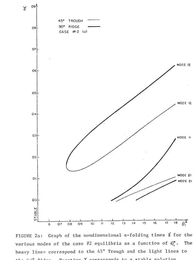
For an example we consider the equilibria and their
stability properties as a function of for the parameter set k=.04, k'=.005,
(
=.22, li=.3, h=.045, G-,=.15, n=1.22 forC
ranging from .06 to .18. (This is a case which we consider in Chapter 5, in which we discuss the time dependent behavior of the model). In Figure 1, we plot the amplitude of the W- component of the equilibria as a function ofG.
For low values of , only the Hadley Solution exists, which is purelyzonal and has no wave amplitude. For Ge>.075, two wavy equilibria appear and for G=,>.105 two more wavy equilibria appear. The upper branch of the first two solutions shall be called the 90ORidge, since the phase of the Mode 11 wave is generally about 90 west of the orographic ridge for the bulk of the values of O considered, while the lower branch will be referred to as the 450Trough for similar reasons. The upper branch of the second pair of solutions shall likewise be
as the Near Hadley solution since it has very low wave amplitude and a high zonal index. (For plots of the
equilibrium flow patterns as they appear in the model, see Chapter 6, on model synoptics).
In Figures 2a and b, we plot the e-folding times of the instabilities of the various equilibria to the four modes of the model. (For this particular case, all the solutions are stable to Mode 22 perturbations, so we need only to consider the other three modes). The 906Ridge and the 45 Trough are considered in Fig. 2a and the remaining three equilibria in Fig. 2b.
We see that on the whole the stability of the equilibria decreases as Gincreases. The primary exceptions to this tendency are the Mode 11 disturbances labeled "orographic". These orographic or form drag instabilities, discussed in
detail by Charney and Straus, are characterized by the lack of an imaginary component in the eigenvalues; thus they are
disturbances which grow in place. All the other instabilities are topographically modified baroclinic disturbances. We note that the Mode 12 disturbance is the most rapidly growing
instability for all the equilibria, with e-folding times generally less than 4 to 5 days. The only exception is the very high growth rates obtained by the Mode 11 orographic
somewhat greater than .14.
It is also interesting to note that the Hadley Solution becomes completely stable to Mode 11 disturbances at G*=.13 since the orographic eigenmode becomes stable and the
baroclinic eigenmode does not become unstable until G,=.14. For some parameter sets, both orographically and
baroclinically unstable Mode 11 eigenmodes exist simultaneously, cf. Charney and Straus (1980).
RECAPITULATION
We have extended the simple highly truncated spectral channel model of Charney and Straus to include both a
topographically forced planetary scale wave and a synoptic scale wave which can directly interact. The model has eight external parameters k, k', , 2, h, G; ,
G,
and n which must be specified before the system can be integrated. We then considered a range of nondimensional values for each of these eight parameters which could arguably correspond to earthlike values. A technique was developed to compute all the large-scale equilibria and their respective stabilities to perturbations on the scale of each of the four modes. We are now ready to investigate the time dependent behavior of the model for general sets of external parameters.5. TIME DEPENDENT BEHAVIOR
We approach the majority of our time dependent
investigations in a similar manner: First we select a set of appropriate external parameters which then remain fixed
throughout the entire process of integration. Once the parameters are chosen, we use the routines discussed
previously to calculate all the equilibria and their
respective stabilities. The model is then initialized at one of its equilibrium states and perturbed by a small Mode 21
( 9',=.002) and Mode 12 ( Y7=.001) disturbance to which all the equilibria are highly unstable. The equations are then
numerically integrated in time steps of 1.5 hours using the N-cycle scheme of Lorenz (1971), with N=4.
The aspects of the time dependent behavior we are most interested in are the periods of quasi-stationarity. As
discussed previously, quasi-stationary behavior is observed to be confined primarily to the planetary scale, which in our simple model is represented by the Mode 11 wave.
Consequently, we can identify the occurrence of a regime or quasi-stationary period simply by observing the behavior of this single wave.
To analyze the time dependent behavior of the Mode 11 wave, we construct phase space plots whose axes are defined by
the streamfunction variables 1' and 941, and observe the motions of this two-dimensional projection of the 20 dimensional model trajectory as a function of time. The occurrence of regimes is then noted by the tendency for the trajectory to be contained within a certain region of phase space for an extended period of time.
Before we actually consider any time dependent
calculations, we briefly discuss the behavior of the flow as anticipated by the multiple flow equilibria theory (MFET). As stated in the introduction, one of the primary assumptions of the MFET is that the synoptic-scale baroclinic instabilties provide a mechanism through which the state of the atmosphere vacillates from one "realizable" equilibrium state to another, where "realizable" equilibria are defined by Charney and
DeVore, Charney and Straus, and Charney et. al. as those equilibria which are quasi-stable to large-scale
perturbations. Implicit in this assumption is that the
effects of the synoptic scales upon the equilibria themselves are minimal. These assumptions imply that the qualitative time dependent behavior of our model is determined by the phase space positions of the equilibria and their respective stabilities to Mode 11 disturbances. In particular, the MFET assumes that periods of quasi- stationary behavior and blocks are intimately tied to the location of the calculated
to aperiodically vacillate between such states.
The most important result of our time dependent experiments is that, for a wide range of the external
parameters, the model atmosphere is observed to aperiodically settle into one of two distinct flow configurations for
extended periods of time. These two preferred states are characterized by the confinement of the Mode 11 components of the trajectory to two distinct regions of phase space,
behavior which we will define as quasi-stationarity in the large-scale Mode 11 wave. Superposed upon these
quasi-stationary large-scale Mode 11 features are erratic eastward propogating synoptic-scale waves with periods on the order of three to five days. This rather remarkable weather regime behavior is best illustrated by the consideration of an example. We select the parameter set
k=.05, k'=.Ol, ( =.2, Ii?= .2,
h=.045, G', =.1, e =.1, and n=1.3,
whose five equilibrium states and respective stabilities to the four modes are given in Table 2.
We can see that the purely zonal Hadley solution (*1) and the low wave amplitude Near-Hadley solution (*2) possess high zonal indexes. The other three solutions possess substantial wave amplitude and lower zonal indexes and are named according to the position of the mid-level wave with respect to the
orography. Two of the equilibria, the Near Hadley solution (*2) and the 90 degree Ridge solution (#3), have easterly
surface flow, N', - G < 0. We also note that even though one of the equilibria is stable and one weakly unstable to Mode 11 perturbations, all of the equilibria are highly unstable to Mode 12 synoptic-scale perturbations. From the form of the eigenmode and the eigenvalue (not shown), it can be
ascertained that the Mode 12 instabilities are all propagating baroclinic disturbances. The only non-propagating orographic instabilities for this particular set of parameters are
Mode 11 perturbations upon the 30 degree Ridge and Near Hadley solutions.
Figure 3a is a plot of the daily position of the
't-~I -component of the trajectory for the first 17 years of the integration period, which is taken as representative of the climatological state of the Mode 11 wave. Though the rather limited range of phases in the climatological state is
in itself noteworthy, the most interesting behavior is not revealed until we compare the climatological state of the model with Figures 3b and 3c. The latter two figures are again plots of the daily position of the N -*-component of the trajectory, but for periods that coincide with the
duration of the two single weather regime events. Figure 3b consists of the 175 day period from time step 20765 to 23564, during which the trajectory remained exclusively in the lower


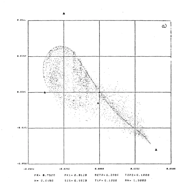


![Degradation Mechanism in La0.8Sr0.2CoO3 [La subscript 0.8 Sr subscript 0.2 CoO subscript 3] as Contact Layer on the Solid Oxide Electrolysis Cell Anode](data:image/gif;base64,R0lGODlhAQABAIAAAP///wAAACH5BAEAAAAALAAAAAABAAEAAAICRAEAOw==)