A Dynamic Programming approach to the Aircraft Sequencing problem

A DYNAMIC PROGRAMMING APPROACH TO THE AIRCRAFT SEQUENCING PROBLEM

by

Harilaos N. Psaraftis

FTL Report R78-4 October 1978

Flight Transportation Laboratory Massachusetts Instittue of Technology

A DYNAMIC PROGRAMMING APPROACH TO THE AIRCRAFT SEQUENCING PROBLEM

ABSTRACT

In this report, a number of Dynamic Programming algorithms for three versions of the Aircraft Sequencing problem are

developed. In these, two alternative objectives are considered: How to land all of a prescribed set of airplanes as soon as possible, or alternatively, how t6minimize the total passenger waiting time. All these three versions are "static", namely, no intermediate aircraft arrivals are accepted until our initial

set of airplanes land. The versions examined are (a) The single runway-unconstrained case, (b) The single runway-Constrained Position Shifting (CPS) case and (c) The

two-runway-unconstrained case. In the two-runway-unconstrained case, no priority con-siderations exist for the airplanes of our system. By contrast, CPS prohibits the shifting of any particular airplane by more than a prespecified number of positions (MPS) from its initial position in the queue. All three algorithms exploit the fact that the airplanes in our system can be classified into a rela-tively small number of distinct categories and thus, realize drastic savings in computational effort, which is shown to be a polynomially bounded function of the number of airplanes per category. The CPS problem is formulated in (b) in a recursive way, so that for any value of MPS, the computational effort

remains polynomially bounded as described above.

All algorithms of this work are tested by various examples and the results are discussed. Implementation issues are

considered and suggestions on how this work can be extended are made.

ACKNOWLEDGEMENTS

This work was supported in part by the Federal Aviation Administration under contract DOT-FA77WA-4007.

The author is particularly indebted to Professors Amedeo Odoni, Christos Papadimitriou and John Devanney for their continuous

assistance. Thanks are also due to Professor Robert Simpson for his comments.

TABLE OF CONTENTS Page ABSTRACT ...--- -TABLE OF CONTENTS -...- - - --...---... ACIOWLEDGEMENTS...---...---.-''.-.--LIST OF FIGURES.--....-....--.-.---...-.-.-.-.-.'.-.--...---LIST OF TABLES...--- ---- ---- *-*-- '--- ---- ---- --- ---- ---- ---INTRODUCTION AND OUTLINE.-.-.-.-.-.-.-.-.-.-.-.-.-.-.-... - - ... PART I: GENERAL BACKGROUND

...-...---CHAPTER 1: Algorithms and Computational Efficiency... 1.0 Introduction: Performance Aspects of Algorithms...

.10 .17 .18 .18

CHAPTER 2:

PART II: THE CHAPTER 3:

1.1 The Concept of NP-Completeness in Combinatorial

Optimization Problems... 23

1.2 Remedies for NP-Completeness...27

The Dynamic Programming Solution to the Travelling Salesman Problem...33

2.0 Introduction...33

2.1 The Dynamic Programming Algorithm...36

2.2 Comparison with Other Approaches...38

AIRCRAFT SEQUENCING PROBLEM (ASP)...43

Aircraft Sequencing: Problem Description...44

3.0 Introduction...44

3.1 Problem Formulation...--47

3.2 Graph Representation of the ASP...49

CHAPTER 4: ASP-Unconstrained Case: Dynamic Programming Solution..... 56

--. 1

TABLE OF CONTENTS (CONT')

Introduction: Dynamic Programming Formulation. Solution Algorithm ... 4.2 Computational Effort and Storage Requirements... 4.3 Computer Runs - Discussion of

CHAPTER 5:

CHAPTER 6:

the Results._{.. . . .. . .} 64

4.4 Directions for Subsequent Investigation... ASP-Constrained Position Shifting (CPS)-Dynamic Programming Solution... 5.0 Introduction: Meaning of CPS... 5.1 Outline of Solution Approach Using Dynamic Programming ---... 5.2 The D.P. Algorithm... 5.3 Computational Effort and Storage Requirements.. 5.4 Computer Runs - Discussion of the Results ... The Two-Runway ASP... 6.0 Introduction: Formulation and Complexity of the Problem ... 6.1 Solution Algorithm... 6.2 Computer Runs - Discussion of the Results ... 6.3 _{Further Remarks on the Two-Runway ASP} .--6.4 Summary of the DP Approach to the ASP .----PART :II: FINAL REMARKS... CHAPTER 7: Conclusions and Directions for Further Research. 7.0 Introduction... 7.1 ASP: Review of the results of this work ... 7.2 ASP: "Dynamic" Case... 7.3 ASP: Multiple Runways... 7.4 ASP: Usefulness of the "Steepest Descent" Heuristic for TPD Minimization ... .... ... 71 ... 73 ... . . 73 -.---. .. 78 ... 83 .. . . .84 ... 86 ... 93 ... 93 ... 97 ... 100 . 107 ...-- 108 ...110 .. .. .111 ... 111 ... 118 ... 120 4.0 4.1 Page ... 56 ... 58 .... 62

TABLE OF CONTENTS (cont'd)

Page REFERENCES

PART IV: APPENDICES...127 APPENDIX A: ASP-Investigation of Group "Clustering"...128 APPENDIX B: ASP-Derivation of the Time Separation Matrix...145 APPENDIX C: ASP-On the "Reasonableness" of the Time Separation

Matrix...149 APPENDIX D: ASP-Equivalence Transformations in Group "Clustering"...154 APPENDIX E: The Computer Programs...167

LIST OF FIGURES

FIig. Page

1.1 Example graph for the MSTP and TSP...24

1.2 Optimal solutions to the MSTP and TSP of the graph Fig. 1.1.. .24

2.1 A 4-node graph and its corresponding cost matrix [d .]...35

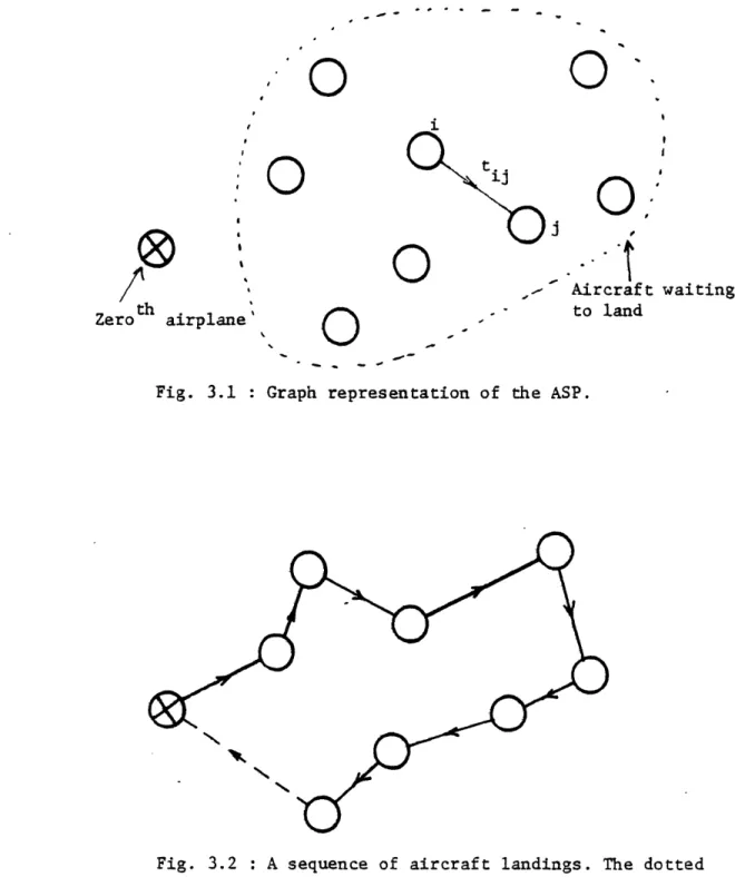
3.1 Graph representation of the ASP...50

3.2 A sequence of aircraft landings...50

3.3 Graph size reduction due to category classifications...54

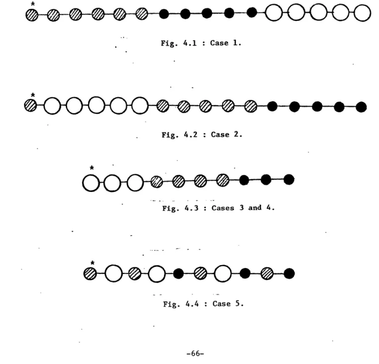
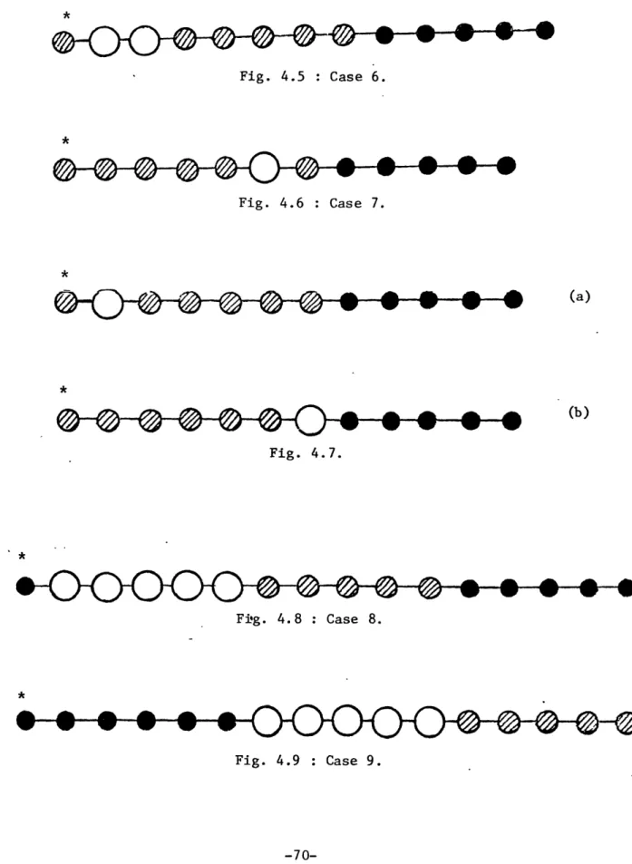
4.1 ASP-unconstrained Case: ASP-unconstrained ASP-unconstrained ASP-unconstrained ASP-unconstrained ASP-unconstrained ASP-unconstrained ASP-unconstrained ASP-unconstrained ASP-CPS ASP-CPS ASP-CPS Case: Case: Case: Case: Case: Case: Case: Case: Case: Casd: Case: Case 1.. Case 2.. Case 3.. Case 1...66 Case 2...66 Cases 3 and 4...66 Case 5...66 Case 6...70 Case 7...70

Further analysis of Case 7... 70

Case 8...70 Case 9...70 ... . . . - - . - - - . - - 88 ... . . . - . . - . - - - - 88 ... . . . - - - - . - - - . 88 4.2 4.3 4.4 4.5 4.6 4.7 4.8 4.9 5.1 5.2 5.3 5.4 5.5 5.6 5.7 6.1 ---- 90 -90 92 92 ... 102

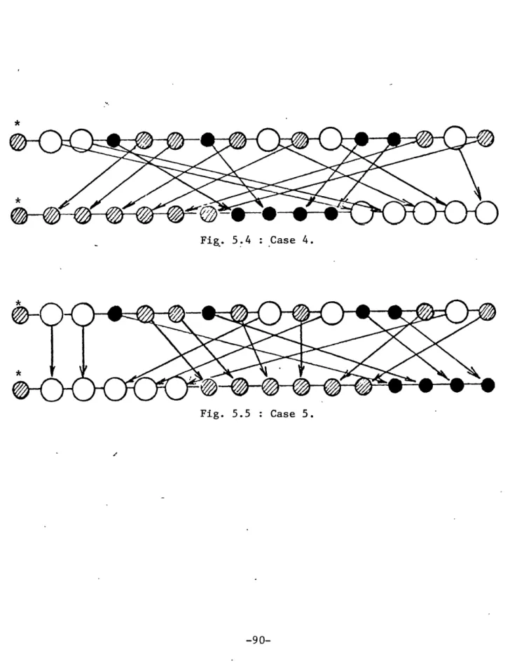
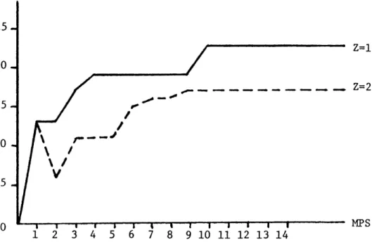
ASP-CPS Case: Case 4... ASP-CPS Case: Case 5... % improvement in LLT with respect to the FCFS discipline % improvement in TPD with respect to the FCFS discipline ASP-Two runway Case: Example...

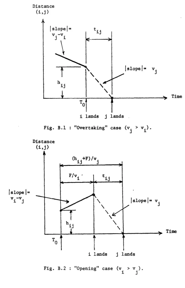
LIST OF FIGURES (CONT'D) Fig. 6.2 6.3 6.4 6.5 6.6 6.7 7.1 A.l A.2 A.3 A.4 A.5 A.6 A. 7 A.8 A.9 A. 10 A. 11 A.12 a. 1 Page Case 1 ... 102 Case 2 ... 102 Case 3 ... 105 Case Case Case ASP-Two runway Case: ASP-Two runway Case: ASP-Two runway Case: ASP-Two runway Case: ASP-Two runway Case: ASP-Two runway Case: ASP-"Dynamic" Case --ASP-Investigation of ASP-Investigation of ASP-Investigation of ASP-Investigation of ASP-Investigation of ASP-Investigation of ASP-Investigation of ASP-Investigation of ASP-Investigation of ASP-Investigation of ASP-Investigation of ASP-Investigation of "Overtaking" Case (v. 4...105 5 ... 105 "clustering": "clustering": "clustering": "clustering": "clustering": "clustering": "clustering": "clustering": "clustering": "clustering": "clustering": "clustering": Results 1 and 2... Result 3... Result 3... Result 4... Results 6 and 7... Result 7... Result 7... Result 8... Results 10 and 11.... Result 12... Result 15... Result 18 ... .105 .114 .131 .131 -131 .131 .136 .136 .136 .136 .140 .140 .140 .140 > v.) ... 148 1 B.2 "Opening" Case (v. > v.)...148 C.1 ASP-Reasonableness of [t..] and consequences...153 D.1 ASP-Equivalence transformations in group clustering...157

group group group group group group group group group group group group

LIST OF FIGURES (CONT'D) Fig. D.2 D.3 D.4 D.5 D.6 D.7 transformations transformations transformations transformations transformations transformations group group group group group group Page clustering...157 clustering ... 160 clustering ... 160 clustering ... 160 clustering...163 clustering...163 ASP-Equivalence ASP-Equivalence ASP-Equivalence ASP-Equivalence ASP-Equivalence ASP-Equivalence

LIST OF TABLES

Table _Page

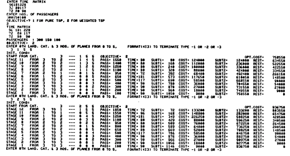
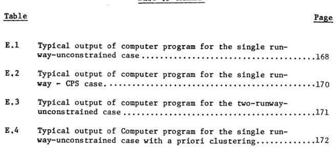
E.1 _{Typical output of computer program for the single}

run-way-unconstrained case...168 E,2 _{Typical output of computer program for the single}

run-way - CPS case...170 E,3 Typical output of computer program for the

two-runway-unconstrained case...171 E,4 Typical output of Computer program for the single

INTRODUCTION AND OUTLINE

This report is excerpted from the author's Ph.D. dissertation "Dynamic Programming Algorithms for Specially Structured Sequencing and Routing Problems in Transportation" (Department of Ocean Engineering, M.I.T., September 1978). Thus, Chapters 1 to 6 as well as Appendices A to D of the report are essentially identical to those of the dissertation. Chapter 7 of the report corresponds to Sections 11.0 to 11.5 of Chapter 11 of the dissertation and Appendix E of the report covers the first half of Appendix E of the dissertation.

The main purpose of this work is to investigate the problem of sequencing aircraft landings at an airport, or what we shall call the

Aircraft Sequencing Problem (ASP). This is a very important problem at the present time, and is currently under investigation by a number of organiza-tions (FAA, NASA, etc.).

Our investigation encompasses the development of analytical models describing the above real-world problem, as well as the design, testing and refinement of novel, specialized and efficient solution procedures tailored to specific versions of this problem. It also includes interpretation of the results of the above procedures and discussion of implementation issues as well as of directions for further research.

In addition to the above, this investigation provides an opportunity to relate this research to some currently "hot" theoretical issues in the areas of computational complexity and algorithmic efficiency and to illustrate

their importance in the area of combinatorial optimization.

is not to be interpreted as a lack of interest for this rapidly growing area of optimization, but rather as an attempt to investigate the

potential savings that may result from exact, specialized solution procedures which exploit the special characteristics (or, what we shall call in this report, the special structure) of the problems at hand.

Now that this attempt has been concluded, our findings in this res-pect are, we believe, interesting and significant.

The material in the report is organized into four parts:

a) Part I presents the necessary background for the investigation to follow.

b) Part II is devoted to the development of Dynamic Programming algorithms for several versions of the ASP.

c) Part III reviews the results of this work and suggests directions for further research.

d) Finally, Part IV includes several appendices with additional technical material on the ASP and a description of the computer programs implementing the algorithms developed in Part II.

Specifically, the organization of the report goes as follows: 1) Part I: General Background

In Chapter 1, we introduce and review the fundamental issues concerning the computational efficiency of algorithms. As a first step, we discuss the generally established classification of algorithms into "efficient" (or poly-nomial") and "inefficient" (or "exponential"). According to this

classifica-tion, an "efficient" algorithm can solve a given problem in running time which is a polynomially bounded function of the size of the problem's input. We argue that for problems of sufficiently large size, "inefficient" algorithms are not likely to be of any practical use. As a second step, we refer to the

For these problems, no "efficient" algorithms are known to exist, but also nobody to date has been able to prove the impossibility of such algorithms. We discuss several remedies to deal with such problems, namely heuristics and exploitation of special structure, if such a

structure exists.

Chapter 2 formulates a famous NP-complete problem, the Travelling Salesman Problem (TSP) and presents a well-known Dynamic Programming approach to solve it. The TSP will be seen to constitute a "prototype" for the Aircraft Sequencing Problem we examine in subsequent chapters.

As expected, the D.P. algorithm for the TSP is an "exponential" algorithm. Also, it is not necessarily the best way to solve this problem in its

general form. It possesses, however, certain characteristics which will be exploited in our specially structured problem later. At this point, we compare the D.P. approach with some other well-established approaches

for the solution of the TSP.

2) Part II: The Aircraft Sequencing Problem (ASP)

In Chapter 3 we formulate an important real-world problem which derives from the TSP and exhibits a special structure that will eventual-ly enable us to solve it in a viable way, the Aircraft Sequencing Problem

(ASP). We describe the physical environment of the problem, that is the near terminal area around airports and we introduce the ASP as a decision problem of the air traffic controller. This problem consists

of the determination of an appropriate landing sequence for a set of airplanes waiting to land, so that some specific measure of performance is optimized. The special structure of the problem is due to the fact that while the total number of airplanes may be substantially large,

these can be "classified" into a relatively small number of "categories" (e.g. "wide-body jets," "medium-size jets," etc.). Another characteristic of the problem, which in fact makes it non-trivial, is that the minimum permissible time interval between two successive landings is far from being constant for all pairs of aircraft categories. Two alternative objectives are considered: Last Landing Time (LLT) minimization and Total Passenger Delay (TPD) minimization. LLT minimization implies that all existing aircraft land as soon as possible. TPD minimization is concerned with minimizing the sum of the "waiting-to-land" times for all passengers in our system, an objective which is identical to the mini-mization of the average-per-passenger delay. The version of the problem which is described in this chapter, is "static," namely no aircraft ar-rivals are permitted (or taken into consideration if they occur) after a point in time t=0.

In Chapter 4 we develop a modified version of the classical D.P. algorithm for the TSP (that was presented in Chapter 2) to solve the

un-constrained case of the single runway ASP. Unun-constrained means that the air traffic controller is not (for the moment) bothered with priority considerations, being free at any step to assign the next landing slot to any of the aircraft not landed so far. The algorithm we have developed evaluates with equal ease either one of the alternative objectives we have suggested in Chapter 3. More importantly however, drastic savings in computational effort are achieved. These savings result from our taking advantage of category classifications. The algorithm exhibits a running time which is a polynomial function of the number of aircraft per

categories but for the ASP this number is small (3 or 4 or, at most, 5). The computer outputs for several cases for which the algorithm was tested, exhibit sufficiently interesting patterns to stimulate further

investiga-tion concerning the underlying structure of the'ASP. Thus, while in most cases, all the aircraft of a given category tend to be grouped in a single "cluster", in other seemingly unpredictable cases this pattern is upset. There are also cases where seemingly negligible changes in the problem input, produce global changes in the optimal sequence. An extensive in-vestigation of these interesting phenomena is left for Appendices A through D.

In Chapter 5, we introduce priority considerationsinto our problem. Specifically, the Constrained Position Shifting rules are introduced. According to these, the air traffic controller is no longer free to

as-sign the next landing slot to any of the remaining aircraft, but is limited to shift the landing position of any aircraft up to a maximum of a prespecified number of single steps upstream or downstream from the initial position of the aircraft in the original first-come, first-serve sequence of arrivals in the vicinity of the near terminal area. This number is known as Maximum Position Shift (MPS) and it is a new input to our problem. An additional input is the (ordered) initial sequence of aircraft. The problem is again assumed "static" with the same alternative objectives as in the unconstrained case. A new D.P. algorithm is developed

incorporating our priority constraints in a way specially suited to the recursive nature of our approach. By contrast to existing complete enu-meration procedures which can deal with CPS problems only for small values of MPS, our algorithm can solve the CPS problem for any value of MPS and

still remain within polynomially bounded execution times with respect to the number of aircraft per category. Computer runs for several cases of this problem have been performed and the results are discussed.

Chapter 6 formulates the problem of sequencing aircraft landings on two identical and parallel runways. We consider again the "static" un-constrained case. The minimization of LLT is seen to constitute a mini-max problem. Our alternative objective is, as before, to minimize TPD.

We see that this problem essentially involves the partitioning of the initial set of airplanes between the two runways, as well as the subse-quent sequencing.of each of the two subsets to each of the two runways, independently of one another. The algorithm we have developed for this problem is a post-processing of the table of optimal values created by a single pass of the unconstrained single runway D.P. algorithm (Chapter 4). Despite the fact that we solve the partitioning subproblem by com-plete enumeration of all possible partitions, the computational effort of the algorithm remains a polynomial function of the number of aircraft per category. Computer runs of this algorithm show some interesting parti-tioning and sequencing patterns. Specifically, while in some cases the composition of aircraft is more or less the same for the two runways, in other cases the partition becomes completely asymmetric. We discuss these and related issues at the end of the chapter.

3) Part III: Final Results

In Chapter 7, we review the main results of this work, suggest directions for possible extensions and address issues on the implementation of the

developed algorithms. In particular, the "dynamic" version of the ASP is seen to constitute a very important extension to this work.

4) Part IV: Appendices

These appendices present additional technical issues related to the ASP. They are organized as follows:

a) Appendix A: Investigation of group "clustering" in the ASP.

b) Appendix B: Derivation of the elements of the time separation matrix in the ASP.

c) Appendix C: Investigation of certain properties of the time separation matrix in the ASP that are connected to group clustering.

d) Appendix D: Development of some equivalence transformations in group clustering and in the case of variable numbers of passengers per air-craft category.

PART I

CHAPTER 1

ALGORITHMS AND COMPUTATIONAL EFFICIENCY

1.0 Introduction: Performance Aspects of Algorithms

An algorithm is a set of instructions for solving a given problem. These instructions should be defined in such a way, so that the following are satisfied:

1) The instructions should be precisely-defined and comprehensive. Thus, nothing should be left to intuition or imagination, and there should be no ambiguity or incompleteness.

2) The corresponding algorithm should be able to solve not just one, but all of the infinite variety of instances of the given kind of problem.

A very simple example of an algorithm is the procedure we use to multiply two numbers. Although not often realized, this procedure con-sists of a sequence of steps. 'each dictating in exact detail the actions

that we should take to solve the problem. Using this procedure we can determine the product of any given pair of numbers.

The nature of an algorithm is such, that it is convenient to represent it in computer language. This convenience, together with the rapid growth in the science and technology of the computer during recent years, have resulted in an increasing effort toward the design and analysis of computer algorithms [AHO 74]*, as well as to the development of solution procedures

for several kinds of problems, that are specifically tailored to computer programming. An example of this approach to optimization and related problems concerning graphs and networks is the excellent work of

Christo-fides [CHRI 75].

The interaction between the theoretical development of an algorithm on the one hand and its computer implementation on the other has been

so strong, that it has now become almost impossible to address the first issue without thinking about the other as well. In fact, a synonym for Ialgorithm" has often been the word "program," which, besides its primary meaning as a set of instructions in computer language, ended up also being

used to describe general as well as specific analytical methodologies: Thus, in the area of optimization we have Mathematical programming, Linear programming, Dynamic programming, etc.

It is conceivable that more than one different algorithms can solve the same problem*. In our multiplication problem, for instance, we can find the product of, say, 24 by 36 by adding 36 times the number 24. We can, of course, apply also our well known multiplication procedure and get the same answer much faster. This elementary example illustrates the fact that certain algorithms are better than others for the solution of a given problem.

For problems of considerable difficulty the above fact becomes very important. For such problems, it is much less important to devise an algorithm that just solves the problem, than to find an algorithm that

*It is also conceivable that no algorithm can be devised for certain prob-blems. This was first demonstrated by Turing in the 1930's[TURl37].

does this efficiently. This is true for all optimization problems and in particular for those where the importance of being able to obtain an optimal solution fast is very high or even crucial.

Subsequent parts of this thesis will be devoted to the examination of such problems and the need for powerful and efficient algorithms will be seen to be apparent. For the moment, we shall introduce some issues regarding algorithmic performance.

Temporarily avoiding being explicit on what is an "efficient" algor-ithm', we start by examining a hypothetical situation: Suppose we have

two different algorithms, A and B, for solving the same instance of a given problem P. A plausible comparison between A and B would be to run both algorithms on the same machine and choose the one exhibiting the

smallest running time (or cost). The disadvantage of this approach is that, conceivably, this comparison will yield different preferences for problems of different size. For example, if the size of the input to P is n (e.g. the number of nodes ina graph*) it may happen that the running

time of algorithm A is equal to 10-n and that of B equal to 2 n. Then ac-cording to the above selection criterion, algorithm B is better than A for n(5, while the opposite happens for n>,. 6.

One way to remove this ambiguity is to base our choice on the ex-amination of what happens for sufficiently large values of the size of the input (n-++o). Using this criterion in the above example, it is clear that algorithm A is "better" than algorithm B. In fact, A will be "better"

* A graph is a collection of points, called nodes, which represent entities, and lines, called links, joining certain pairs of the nodes and represent relationships between them. An elementary knowledge of concepts such as thisis assumed of the reader.

than B even if one uses A on the slowest computer and B on the fastest, for sufficiently large values of n.

In this respect, we may note that any algorithm whose running time is a polynomial function of the size of the input is "better" than any algorithm whose running time is an exponential function of the size of the input, irrespective of what computers these algorithms are run on. Computer scientists have more or less agreed that algorithms that consume time which is exponential relative to the size of the input are not practically useful [LEWI 78). In that spirit, these algorithms have been characterized as "inefficient". By contrast, an "efficient" algor-ith is said to be one whose running time grows as a polynomial function of the size of the input.

It would perhaps be useful to make several remarks concerning this concept:

1) There may be algorithms whose running times are non-deterministic. That is, one may not know beforehand exactly after how many steps the algorithm will terminate, this depending in an unknown fashion upon the values of the particular inputs. If this is the case, it is important to distinguish between worst-case performance and average performance of the algorithm, since these two may be very different. For a given size of the problem's input, an upper bound for the algorithm's running time may be obtainable. The worst-case performance occurs for those instances of the problem that make the algorithm's running time reach this upper bound

(for many non-deterministic algorithms the generation of such worst-case instances, is an art in itself). On the other hand, the algorithm will not be

used only in worst-case instances, but also in other, more easy cases. The aspect of the algorithm's performance that emerges from this consideration

is its average performance.

There seems to be no definite answer to the question of which of the two aspects is more important. Although it would certainly be de-sirable to have a strong "guarantee" for the performance of an algorithm (and such a guarantee can come only from a good worst-case performance), there may be some "controversial" algorithms which have bad worst-case performances and exceptional average performances. In fact, the best known example of such a controversial non-deterministic algorithm is none other than the famous Simplex method introduced by George Dantzig in Linear Programming [DANT 51, DANT 53]. The controversy lies in the fact that while on the average the running time of this algorithm is proportional to a low power polynomial function of the size of the input, carefully worked out instances of Linear Programs, show that Simplex may require an exponential amount of time [ZADE 73]. Thus, a yet unsolved enigma to mathematical programmers is the question of why an algorithm as "bad" as

Simplex(in the sense that there is no polynomial performance guarantee) turns out to work so exceptionally well [KLEE 70].

2) Examining the performance of an algorithm asymptotically as we did for algorithms A and B earlier has the advantage of making the speed of the algorithm its own intrinsic property, not depending on the type of computer being used, or on possible technological breakthroughs in com-puter design and speed. However, this asymptotic behavior should be studied with caution. A hypothetical and extreme example where the poly-nomial/exponential discrimination may be illusory is if we compare a

de-80

terministic algorithm whose running time goes, say, as n with a deter-ministic algorithm for the same problem whose running time goes as 1.001n

"efficient" (polynomial) and reject the second because it is "inef-n80

ficient" (exponential). In fact, it is true that imn n = 0, n ae sn+m 1.001

but the values of n for which 1.001 > n are so large, that they most probably lie outside the range of practical interest.

This example was hypothetical and extreme. In fact, all known poly-nomial algorithms for graph-theoretic problems grow much less rapidly

80 2

than n (most known algorithms of that category grow as n, nlogn, n , n3 and at most n 5). In addition, all known exponential algorithms grow much more rapidly than 1.001n (for'example, there are algorithms growing like 2 n). Therefore, in subsequent sections we shall adhere to the

de-finition of computational "efficiency" given earlier. We shall excersise caution however, and think twice before "accepting" an algorithm just be-cause it is polynomial or "rejecting" it just bebe-cause it is exponential.

1.1 The Concept of NP-Completeness in Combinatorial Optimization Problems. Among problems where the issue of computational efficiency is ex-tremely important are those belonging to the general category of combina-torial optimization problems. Since the Aircraft Sequencing Problem which we will be studying throughout this report belong to that

general category, it is important to examine the issue of computational efficiency from a slightly more specialized point of view.

The two examples which follow constitute well known combinatorial optimization problems and will provide motivation for subsequent parts of the thesis:

Let G be the graph of Fig. 1.1. We assume that if we use a parti-cular link of G, we pay the corresponding cost ($1 for link AB, $2 for link BC, etc.). Missing links have infinite cost (e.g. AC).

Fig. 1.1.

(MSTP) (TSP)

We consider the following problems concerning G:

Problem 1 (Minimum Spanning Tree Problem or MSTP): Use as many links of G as necessary, to connect* all nodesof G at minimum cost. Problem 2 (Travelling Salesman problem or TSP): Find a tour in G of minimum cost. _{(A tour is a sequence of visits to all nodes of} the graph exactly once,which returns to the initial node.)

Before proceeding with more details, we exhibit the optimal solutions to these two problems in Fig. 1.2. We may.at first glance note that

the two problems above seem very similar in structure and we might also expect that they are very similar with respect to solution precedures and computational effort required, as well.

Surprisingly enough however, it turns out that the MSTP is one of the easiest problems known in the field of combinatorial optimization. By _{contrast, the TSP is one of the toughest ones.}

Many "efficient" algorithms exist for the MSTP. The fastest for arbitrary link costs and a general graph structure is the one by Prim

[PRIM 57], in which _{the runniig time goes as n (n: number of nodes of}

the graph). _{For graphs where the nodes are points in a Euclidean plane} and link costs are proportional to the Euclidean distance between the two nodes, one can do even better than that. The algorithm of Shamos and Hoey

[SHAM 75] _{exhibits a computational effort that goes as nlogn.}

By contrast, no "efficient" algorithm _{has been developed for the TSP,} despite the fact that the problem has been a very popular target for am-bitious mathematicians and operations researchers for several decades.

* _{Connectivity means to be able to reach every node of the graph from}

All algorithms that exist today for the TSP are "inefficient." These failures led to the subsequent classification of the TSP into a relative-ly wide class of similarrelative-ly notorious problems, the so called NP-complete problems*. This class of problems has a unique property: If an "ef-fient" algorithm exists for just one of them, then "efficient" algor-ithms exist for all of them. A consequence of this property is that if it is proven that just one of these NP-complete problems cannot have an "efficient" algorithm, then none of these problems can [KARP 75].

As a result of the above ideas, the effort of researchers on-the subject, has been channeled toward two opposite directions: Either to-ward finding an "efficient" algorithm for a specific NP-complete problem,

or, toward proving that this is impossible. The efforts in this latter direction are a natural consequence of the repeated failures in the former.

Unfortunately, however, these new efforts have so far had the same fate as the previous ones. In other words, no one to date has managed to prove the impossibility o-f devising polynomial algorithms for NP-com-plete problems and this leaves the status of this case open. Incidental-ly, it has also been realized that there are some other problems which are one step closer to "darkness" than NP-complete problems are: These are problems for which nobody knows if they are NP-complete or not. (The. problem of Graph Isomorphism and the general Linear Programming problem belong to this category.)

Returning to NP-complete problems, current opinion is divided. Some researchers strongly suspect that no "efficient" algorithm can be

constructed for them. Others speculate that these problems will even-tually yield to polynomial solutions. Finally there are those who be-lieve that the resolution of this question will require the development of entirely new mathematical methods. [KARP 75, LEWI 78].

Some other remarks are worthwhile:

1) The solution of the TSP of the previous example may have seemed tri-vial because there were only two feasible tours in the graph of Figure 1.1. It is important though to bear in mind that the number of

feas-ible tours in a complete graph with symmetric distances grows ex-plosively with the size of the problem, being in fact equal to

(n-l)! As for graphs with missing links like the one we examined, it is conceivable that not even one feasible tour exists. Moreover, the problem of finding whether a given graph has a TSP tour is, in itself, a NP-complete problem.

2) Referring once again to the possibility that the number of feasible solutions to a combinatorial optimization problem may be explosively large, this fact should not be automatically associated with the "tough-ness" of that problem. As a matter of fact the number of feasible so-lutions to the MSTP for a complete graph of n nodes is even larger than to the equivalent TSP! (This number is equal to nn-2; a biblio-graphy of over 25 papers proving this result is given in [MOON 67].) 1.2 Remedies for NP-Completeness

There are several things one can do if faced with a NP-complete prob-lem, besides quitting:

1) Accept the high computational cost of an exponential algorithm. 2) Compromise on optimality.

3) If the problem at hand has a special structure, try to take ad-vantage of it.

The first alternative may be viable only under limited circumstances. Excessive storage or CPU time requirements are the most common character-istics of an exponential algorithm even when the size of the problem ex-amined is of moderate magnitude. Thus, large scale problems or problems requiring real-time solutions may make the use of such algorithms not attractive and even prohibitive.

The second alternative is very interesting. The basic philosophy behind it is the following: "If it is so expensive to obtain the exact optimal solution of a problem, perhaps it is not so expensive to obtain a "reasonably good"* solution. In any event, the exact optimal solution may not be so terribly important because the mathematical problem itself is an abstraction and therefore an approximation of the real-world prob-lem."

Following this line of logic, various techniques have been developed in order to obtain "reasonably good" solutions to a given optimization problem, requiring only a fraction of the computational effort required

to obtain the exact optimal solution.

A major reason for adopting this approach has been the anticipation and subsequent verification of the fact that many algorithms produce a "reasonably good" solution quite rapidly but spend a disproportionate amount of computational effort for closing the remaining narrow gap

be-tween the cost of this "reasonably good" solution and the cost of the exact optimal solution. This is particularly common with algorithms *We shall give an explicit interpretation of this term later.

which produce one feasible solution per iteration and subsequently move to another "improved" feasible solution (according to some rigorous or

heu-ristic criteria), until no further improvement is possible. (It should be noted that not all optimization algorithms are of this hill-climbing

or hill-descending nature.) In these cases, it may often be relatively easy to improve upon a "bad" initial feasible solution (hence the rapid generation of "reasonably good" solutions at the beginning), but hard to improve upon a "reasonably good" solution (hence the substantially greater amount of computation in order to make the last small improvements needed to reach the exact optimum).

Thus, we can immediately see a way to construct an algorithm that only produces a "reasonably good" solution: take an algorithm of the above form and operate it until some termination criteria are met. These termination criteria may be one or more of the following:

First, there may be a "resource" constraint, which is translated to limits in the number of iterations, or in CPU time, cost, etc. If this criterion is followed, the algorithm terminates upon exhaustion of the available resource.

Alternatively, a criterion may concern the quality of the best solu-tion found so far. The algorithm then terminates if this solution is "reasonably good." Different people may interpret the term "reasonably good" in different ways. One of the interpretations usually adopted is the following: A "reasonably good" solution is defined as one whose cost provably cannot exceed the (still unknown) minimum total cost of the

For example one might consider as a "reasonably good" solution one whose cost is within 10% of the optimal cost.

Branch-and-bound algorithms are one class of non-deterministic ex-ponential algorithms which are tailored to incorporate such tolerances from optimality, besides their ability to produce also exact optimal so-lutions, given sufficient time. It is unfortunate that it is not possible

to drop the running times of these algorithms to polynomial by sufficient-ly relaxing the optimality requirements.

By contrast, it may be possible to accomplish this exponential-to-polynomial reduction in the so-called heuristic algorithms. These are procedures using arbitrary rules in order to obtain a "reasonably good" solution. These rules may be anything from "common sense,""intuitive" or even "random" courses of action, to more elaborate procedures, some-times employing separate optimization algorithms (drawn from other prob-lems) as sub-routines. The very name of a "heuristic" algorithm suggests

that the algorithm is not a rigorous procedure for reaching the exact optimum, but rather a set of

empirical

an acceptable solution and more hopefully the optimal solution itself.

A solution produced by a heuristic algorithm will be in general sub-optimal. A heuristic algorithm may or may not possess a performance guarantee in the sense that the cost of its solution is guaranteed to be within prescribed limits with respect to the exact optimum.

Concerning the TSP, Christofides [CHRI 76] has recently developed a heuristic polynomial algorithm which guarantees solutions of cost no more than 150% of that of the optimal solution.

carefully worked-out specific problem instances [FRED 77]. It is inter-esting to note that the specific problems for which this happens have a Euclidean cost structure, structure which could conceivably be exploited

to get better results. The fact that not even a heuristic algorithm can guarantee TSP solutions with cost deviations from optimality of less than 50% without requiring exponential running times, is a further indication of the inherent toughness of this problem. It should be pointed out however that 50% is a worst-case performance. The average performance of

this algorithm has been astonishingly good (solutions average cost devia-tions of 5-10% from optimality) and this is a further indication that worst-case performance should not be confused with average performance,

since these two may diffet substantially.

As a third remedy to NP-completeness, we come to what will be seen to constitute a central concept in this investigation This concept can be broadly named as "exploitation of special structure."

We have already briefly mentioned an example where the special

structure of a problem could be used to solve the problem more efficiently: In the MSTP, the very fact that the graph may be Euclidean, can be used

2

to drop the order of computational effort from n to nlogn. By contrast, no similar improvement can be realized for the TSP. In fact, the Euclidean Travelling Salesman Problem is itself NP-complete (PAPA 77].

Similar or more spectacular refinements of general-purpose algorithms to fit specialized problems have constituted a major topic of research in the area of mathematical programming. These "streamlined" versions of the general-purpose algorithms can perform the same job as the latter, but much more efficiently. Examples of this can be found in the plethora

of specialized algorithms in use for many network problems in tion, such as maximum flow, shortest path, transshipment and transporta-tion problems [DIJK 59, DINI 70, EDMO 72, KARZ 74]. These problems are in essence Linear Programs and can be in principle solved by the Simplex method which we have already mentioned earlier. But it turns out that

these specialized algorithms are so successful, that using Simplex instead of them can be characterized as a waste of effort despite Simplex widely

recognized success. What essentially has been achieved through the ex-ploitation of the special structure of these problems (and of many others) is that the algorithms that have been developed for the problems are polynomial.

CHAPTER 2

THE DYNAMIC PROGRAMMING SOLUTION TO THE TRAVELLING SALESMAN PROBLEM

2.0 Introduction

It will be seen that the Aircraft Sequencing Problem which will be examined in subsequent chapters of this report is closely related to the classical TSP. Differences do exist with respect to objective functions, special constraints and other more subtle aspects. Neverthe-less, one should be able to detect a TSP "flavor" in the ASP.

It seems therefore appropriate at this point to examine how one can solve the TSP. In particular, the classical Dynamic Programming Approach

to the TSP will provide the necessary background and motivation for the more specialized and sophisticated solution algorithms which will be de-veloped later.

In the general formulation of the TSP we shall assume that we are dealing with a directed, complete, and weighted graph G of N nodes.

Directed means that the lines joining pairs of nodes are themselves directed. These will be called arcs (e.g. arc (i,j) is a line from node i to node

j)

Complete means that for every ordered pair of distinct nodes (i,j) there exists an arc from i to

j.

Weighted means that every arc (i,j) is assigned a number, called interchangeably distance, separation or cost, d... It is not necessary that the graph is symmetric i.e. that d.. = d... Also, the cost to go from a node i to another node j of the graph, will depend on what other intermediate nodes will be visited. d.. is the cost of going from i to

i3

j directly, so this cost is sometimes called one-step cost between i and

j

j

j,

1.3 IJ

latter matrix satisfies the so-called triangle inequality, i.e. d. <d +d .

13~ ik

kJ

for all (i,

j,

be-tween i and j.

We will also assume that if a graph is not complete, i.e. certain arcs are missing, then the cost of these arcs is infinite. Thus, in ab-sence of loops, we can put d = 0 for every node i.

An example of a 4-node graph with its corresponding cost matrix is given in Fig. 2.1

The Travelling Salesman Problem then calls for finding a sequence of nodes {L, L₂, LN, LN+1} which forms a tour, so that the total cost

N

associated with it ( dL L

)

j=l

j'

j+1

a tour, +1e L .

*It is possible to construct [d!.} from [d..] in time proportional to N3 [FLOY 62, M4URC 65]. 1

2 4 6 43 00 3 oo 4 2 -c 5 7 [d..]. = d3 6 G - 0 2 2. 1 4o

Without loss of generality we can specify an arbitrary starting node therefore put L1 = LN+ = node 1.

2.1 The Dynamic Programming Algorithm.

We now present the Classical Dynamic Programming Approach for solving problems of this kind. This method is due to Held and Karp [HELD 62].

A stage in the TSP involves the visit of a particular node. It can be seen that the TSP problem above has N+l stages: At stage 1 we are at

the initial node 1. At stage 2 we move to another node and so forth until we return to node 1 at stage N+l.

The information on which we shall base our decision on what node to visit in the next stage n+l, given that we currently are at stage n, is described by the following state variables:

L: the node we are currently visiting.

k k 2,...kN a vector describing what nodes have been visited so far. By definition:

k.

= 0 if node

j

has been visited

By convention, at the beginning of our tour we are at node 1 but since we have to visit this node again at the end, we put k =1.

We also define the optimal value function V(L, k ₁, ... , kN) as the minimum achievable cost to return to node 1 passing through all unvisited

nodes, given our current state is (L, k , ... , k

It is not difficult to see that the difinition of V above implies the following optimality recursion, also known as Bellman's principle of optim-ality [BELL 60]:

V(Lk 1 , ... , k

)

where

X={1} if k 2=k 3 ...=k N=0 and kl=l _{(2. 2)} i: i#l and k.=1} otherwise

k. -1(if.j)

and k' k 1 if (2.3)

k otherwise

In (2.2), the set X of potential "next" nodes is described mathemat-ically and in (2.3) the k-vector of a "next" node x'of X is derived from

(L, k ,...,kN). Two facts are clear: 1) At the end of the tour, V is zero.

So V(1,0,...,O)=O. (2.4)

2) The total cost of the optimal solution is given by the value of V(ll,...,1).

To compute this value we use the technique called backward recursion. According to it, we evaluate (2.1) using (2.2) and (2.3) for all

combina-tions of (L, k 1, ... , kN) in -the following manner: We start from

L=l, kl=...=kN=0 where (2.4) applies and then we move to lexicographical-1y greater* values of the k-vector, each time examining all values of L

*A vector (a1,. a N) is said to be lexicographically greater than another vector (bi,... ,bN) if either:

(a) _{a,> b,}

or (b) there exists an index n between 1 and N such that a. = b. for all lj(n and a n> b .

For example, (1,0,0) is lexicographically greater than (0,1,1) because of ('a) and (1,0,1) is lexicographically greater than (1,0,0) because of (b).

from 1 to N. Each time we apply (2.1) we store two pieces of information: First the value of V. Second, what has been our best choice as to what node to visit next. We store this last item in an array NEXT (L, k ,...kN. This array will eventually serve to identify the optimal tour. This

iden-tification takes place after the backward recursion is completed, i.e. after state (1,1,.. .,l) has been reached.

We know that we are initially at node 1 and our state is (1,1,...,1). The best next node is given by the value of NEXT (11,...,1). Supposing for the sake of arguement that this is equal to 3, this means that our state becomes now (3,1,1,0,1,...,1). The best next node is given by the

corresponding value of NEXT and so forth until, after N steps, we arrive back to node 1 and our state becomes (1,0,0...,&).

2.2. Comparison with Other Approaches

We can see that the computational effort associated with this approach grows quite rapidly as N increases, but still far more slowly than the

factorial function associated with a complete enumeration scheme.

N

In fact, (2.1) will be used a number of times of the order of N.2 The reason is that each of the k's can take two values (0 or 1) and L can

take N values (1 to N). Equivalent amounts of memory should be reserved for each of the arrays V and NEXT. This quite rapid growth makes this ap-proach not practical for the solution of TSP's in graphs of more than

about 15 nodes. By contrast, other exact approaches have been shown to be albe to handle TSP's of about 60-65 nodes [HELD 70, HELD 711, while

several heuristic algorithms handle TSP's of up to 100-200 nodes [LIN 65 LIN 73, KROL 711.

It becomes clear therefore that some explanation should be offered here concerning the purpose of presenting the Dynamic Programming

ap-proach.

One perhaps evasive answer to that question is to state that the reasons for which the Dynamic Programming approach has been introduced will eventually become clear in subsequent chapters of this report.

In fact it will turn out that this approach, in the form of more sophis-ticated algorithms, will prove itself useful in tackling the Aircraft Sequencing Problem.

Nevertheless, we can also state a priori some features of the Dynamic Programming approach that make it particularly advantageous by comparison to other approaches.

The first feature concerns the versatility of this approach with res-pect to the form of objective functions that can be handled. The only requirement concerning the form of objective functions suitable for Dynamic Programming manipulation is that of separability: As this tech-nique is used in multi-stage problems, one should be able to separate the cost corresponding to a stage into the cost corresponding to a sub-sequent stage and the "transition" cost to go from the former stage to

the latter. This separation is not restricted to be additive.

Let us state at the outset that this separability requirement may become very restrictive and even prohibitive if certain forms of ive functions are to be considered. For example, if a quadratic object-ive function is used, then the manipulations required to bring this

func-tion to a separable form, will eventually increase the computafunc-tional effort of the procedure much faster thanof a linear objective function.

Despite this restriction, there still remain several forms of ob-jective functions that can be separated, in addition to the one examined in the "classical" version of the TSP presented above (minimize total cost of tour). We shall have several opportunities to examine these al-ternative forms of objective functions later on. For the moment, for motivation purposes we will present one of them:

Consider the following variation of the TSP: A tour is to be executed by a bus which starts from node 1 carrying a number of passengers. Each of these passengers wishes to be delivered to a specific node of the graph. After completion of all deliveries, the bus has to return to node 1. During the trip, each passenger will "suffer" an amount of "ride time" into the bus till his delivery. What should be the sequence of bus stops which minimizes the sum of ride times (or, equivalently, the average ride

time)?

It should be noticed that due to the different form of the objective function, this problem is not the same as the classical TSP seen earlier and in general the optimal solutions to these two problems will not be identical.

In fact, the problem we have just presented belongs to the general category of "mean finishing time" minimization scheduling problems, which unfortunately, are also NP-complete. A more general version of the veh-icle routing version of this problem has been studied in detail in IPSAR 78]. A generalized version of this objective function will also be studied in

Part II.

The important remark, however, at this stage of our presentation is that Dynamic Programming can handle this new form of objective function

with the same ease as it can handle the previous one, being in addition able to consider any linear combination of these two objective functions.

By contrast, other approaches more successful than Dynamic Program-ming in solving "classical" TSP's, fail completely if alternative forms of objective functions like the one above are considered. An example is the node penalty/subgradient optimization/branch-and-bound approach by the same authors who introduced the Dynamic Programming approach for the TSP. Held and Karp in [HELD 70, HELD 71] have presented an algorithm, able to handle TSP's of 60-65 nodes. It is perhaps not fully appreciated that a critical factor in the success of that approach is the form of the objective function itself. Specifically, Held and Karp ingenuously observed that the identity of the optimal solution to the TSP will not change if an arbitrary set of "penalties" is imposed on all nodes of the graph (so that in addition to the cost incurred in using a particular link of the graph, we also have to pay apenalty for each node we visit). Based on that observation the authors subsequently developed a procedure to

identify the combination of node penalties which will enable one to obtain the TSP solution directly from the equivalent MSTP solution.

With respect to this approach, it turns out that the above fundamental observation of the authors simply does not hold if one is examining an

objective different from the classical one. So one is immediately forced to reject this approach if these alternative objectives are examined.

The same observation holds for other approaches including several heuristic algorithms. In particular, the recent ingenuous algorithm of

Christofides [CHRI 76] cannot be applied if other than classical objectives are examined.

The above argument does not mean that there do not exist specialized algorithms for tackling these alternative objectives; in fact such algor-ithms do exist [IGNA 65, VAND 75]. Rather, the purpose of the discussion was to emphasize the flexibility of the Dynamic Programming approach

re-garding certain alternative forms of objectives.

Other features that make the DP approach attractive are the relative ease in computer coding, the capability of examination of specialized con-straints and an effective "re-optimization" ability.

It is however premature to get into details concerning these positive and some inevitable negative aspects of the technique at this point. We shall have several opportunities to do this in parallel with the examina-tion of the specific problems which will be presented subsequently.

PART II

CHAP-TER 3

AIRCRAFT SEQUENCING: PROBLEM DESCRIPTION

3.0 Introduction

It was mentioned in Part I that certain combinatorial optimization problems exhibit structures, whichif adequately exploited, may lead to

the development of "specialized" algorithms solving these problems much more efficiently than a general-purpose algorithm could do.

Following this philosophy, the purpose of Part II is to introduce and discuss a version of the Aircraft Sequencing Problem (ASP), as well

as to develop a "specialized" algorithm for it. The above problem will be seen to be directly related to the Travelling Salesman Problem (TSP) already introduced in Part I, being in fact itself NP-complete. Never-theless, the structure of this problem is such, that, through specially tailored algorithms, drastic.computational savings can be realized over the effort needed to solve the problem with the classical Dynamic Program-ming algorithm (also described in Part I). Moreover, the same structure will be shown to allow the inclusion of a special kind of priority

con-straints, the Constrained Position Shifting rules. We shall examine these and other issues in detail throughout this Part of the report.

Before presenting the mathematical formulation of the ASP let us take a brief look at the real-world problem:

During peak periods of traffic, the control of arriving and departing aircraft in an airport's near terminal area becomes a very complex task.

The modern air traffic controller must, among other things, see to it that every aircraft in that high density area, either waiting to land or preparing to take off, maintains the required degree of safety. The same person also has to decide what aircraft should use a particular run-way, at what time this should be done and what manoeuvres should be

ex-ecuted to achieve this. The viable accomplishment of such a task becomes more difficult in view of the fact that aircraft are continuously entering

and leaving the system and that at peak periods, the demand for runway utilization may reach, or even exceed the capabilities of the system. It is at such periods that excessive delays are often observed, resulting in passenger discomfort, fuel waste and the disruption of the airlines' schedules. Under such "bottleneck" conditions, an increase in collision risk can logically be expected as well. The interaction between delay and safety goes also in the opposite direction: Because of safety con-siderations, the sequencing strategy used by almost all* major airports of the world today is the First-Come-First-Served (FCFS) discipline. For reasons which will become apparent below, this strategy is very like-ly to contribute to the occurrence of excessive delays.

The minimization of delay or some other measure of performance** related to passenger discomfort, without violation of safety constraints is certainly a desirable goal. This goal is, at least theoretically, achievable, for the following reasons:

* London's Heathrow Airport is an exception: A more sophisticated, com-puter assisted process is used there. [BONN 75.]

**Explicit definitions of these measures of performance will be given as soon as we formulate our version of the problem.

First, safety regulations state that any two coaltitudinal aircraft must maintain a minimum horizontal separation, which is a function of

the types and relative positions of these two aircraft.

Second, the landing velocity of an aircraft will not be in general the same as the landing velocity of another aircraft.

A consequence of the variability of the above parameters (minimum horizontal separation and landing velocities) is that the minimum

permis-sible time interval between two successive landings is a variable quantity. Thus, it may be possible, by rearrangement of the initial positions of the aircraft, to take advantage of the above variability and obtain a landing sequence that results in less delay than the FCFS discipline. In fact, an optimal sequence does exist; it is theoretically possible to

find it by examining all sequences and select the most favorable one. The above argument holds only as far as the potential for improvement over the FCFS discipline is concerned. How to find, and, equally

importan-ly, how to implement an optimal - sequencing strategy is another story. The method suggested above fo'r the determination of the optimal sequence is safe, but extremely inefficient, because the computational effort as-sociated with it is a factorial function of the number of aircraft and it will not be possible to evaluate all the combinations in a short time interval (as the nature of this problem demands), even on the fastest computer*.

It should be pointed out that while the main factor that suggests the existence of an optimal landing sequence is the variability of the *With only 10 aircraft, we would have to make 3,628,800 comparisons and

with 15 aircraft 1,307,674,368,000 comparisons! Real-world problems, may involve the sequencing of 100 or more aircraft.