HAL Id: hal-01609011
https://hal.sorbonne-universite.fr/hal-01609011
Submitted on 3 Oct 2017HAL is a multi-disciplinary open access
archive for the deposit and dissemination of sci-entific research documents, whether they are pub-lished or not. The documents may come from
L’archive ouverte pluridisciplinaire HAL, est destinée au dépôt et à la diffusion de documents scientifiques de niveau recherche, publiés ou non, émanant des établissements d’enseignement et de
On the Perception of Audified Seismograms
Lapo Boschi, Laurianne Delcor, Jean-Loic Le Carrou, Claudia Fritz, Arthur
Paté, Benjamin Holtzman
To cite this version:
Lapo Boschi, Laurianne Delcor, Jean-Loic Le Carrou, Claudia Fritz, Arthur Paté, et al.. On the Perception of Audified Seismograms. Seismological Research Letters, Seismological Society of America, 2017, 88 (5), pp.1279-1289. �10.1785/0220170077�. �hal-01609011�
On the perception of audified seismograms
1
Lapo Boschi
1,5, Laurianne Delcor
2,6, Jean-Lo¨ıc Le Carrou
3,
2
Claudia Fritz
3, Arthur Pat´e
4, and Benjamin Holtzman
43
1
Sorbonne Universit´es, UPMC Univ Paris 06, CNRS, Institut
4
des Sciences de la Terre de Paris (iSTeP), 4 place Jussieu
575005 Paris, France
62
Laboratory of Vibration and Acoustics, 69621 Villeurbanne,
7
France
83
Sorbonne Universit´es, UPMC Univ Paris 06, CNRS, Institut
9
Jean Le Rond d’Alembert, ´equipe LAM, 4 place Jussieu 75005
10Paris, France
114
Lamont-Doherty Earth Observatory, Columbia University,
12
New York, U. S. A.
135
ALSO AT: Sorbonne Universit´es, UPMC Univ Paris 06,
14
CNRS, Institut Jean Le Rond d’Alembert, ´equipe LAM, 4
15place Jussieu 75005 Paris, France
166
ALSO AT: Airbus Helicopters, France
May 22, 2017
18Abstract
19Recordings of the Earth’s oscillations made by seismometers, following earth-20
quakes or other geophysical phenomena, can be made audible by simply 21
accelerating and playing them through an audio reproduction system. We 22
evaluate quantitatively the possibility of using such acoustic display of seis-23
mic data for practical applications. We first present to listeners examples 24
of two categories of data, based on geophysical parameters (the geometry of 25
the seismic fault; the terrain–oceanic or continental–sampled by the propa-26
gating seismic wave) that are not revealed to them. The listeners are then 27
asked to associate each of a set of audified seismograms, that are presented 28
to them binaurally, to either one of the two categories. After this exercise, 29
they are asked to define the features of audified signals that helped them in 30
completing this task. A subset of the listeners undergo a training session, 31
before taking one of the tests for a second time. While the number of listen-32
ers is too small for a definitive statistical analysis, our results suggest that 33
listeners are able, at least in some cases, to categorize signals according to all 34
the geophysical parameters we had chosen. Importantly, we clearly observe 35
that listeners’ performance can be improved by training. Our work opens 36
the way to a number of potentially fruitful applications of auditory display 37
to seismology. 38
Introduction
39Auditory display, or “sonification” of scientific data has been applied suc-40
cessfully to research topics in several disciplines [e.g. Cowen, 2015]. Seismic 41
data analysis naturally lends itself to audification: a particularly simple form 42
of sonification which consists of accelerating seismic signals (whose frequency 43
is lower than that of audible sound) before playing them through an audio 44
reproduction system. Auditory display of seismic data was first explored dur-45
ing the Cold War, when the ability to distinguish underground nuclear tests 46
from natural earthquakes acquired a political relevance [Speeth, 1961; Frantti 47
and Leverault, 1965; Volmar , 2013]. Audification was eventually discarded, 48
in this context, in favour of seismic-array methods [Volmar , 2013]; in recent 49
years, however, it has been revived by seismologists, mostly for purposes of 50
teaching and dissemination [e.g. Dombois and Eckel , 2011; Kilb et al., 2012; 51
Peng et al., 2012; Holtzman et al., 2014; Tang, 2014]. Our own experiments 52
[Pat´e et al., 2016, 2017] have convinced us that it is a valuable and inspi-53
rational tool for the analysis of seismic data in many contexts. We suggest 54
that it might also soon find more specific, e↵ective research applications. 55
This study attempts to contribute to the quantitative analysis of the 56
human auditory system’s response to audified seismic data. As researchers 57
peruse data via auditory display, the implicit assumption is made that they 58
are capable of recognizing patterns and completing some related tasks by 59
hearing. We question this assumption for the case of audified seismic data, 60
and thus begin to evaluate what can be achieved by audification that is 61
not already implemented through “traditional” techniques in seismic data 62
analysis. Both the early work of Speeth [1961] and the recent e↵orts by our 63
group [Pat´e et al., 2016] indicate that listeners can detect meaningful clues 64
in audified seismic signals, and thus categorize the signals according to such 65
clues. Pat´e et al. [2016] showed that the categories formed by the listeners 66
can be associated with several geophysical parameters, but could not entirely 67
distinguish the e↵ects of individual parameters (e.g., source-receiver distance, 68
geological properties of the terrain at the receiver and between source and 69
receiver, etc.) from one another. We present here a di↵erent approach to 70
the analysis of audified data: listeners are asked to complete a constrained-, 71
rather than free-categorization task, on two sets of data, each controlled by a 72
single geophysical parameter (Earth structure in the area where the recorded 73
seismic waves propagate; focal mechanism of the source). The listeners’ 74
performance in auditory analysis is compared with their performance in a 75
similar task, completed via visual analysis of analogous data. We consider 76
the visual analysis of a plot to be a “traditional” task that most individuals 77
with some scientific background are, to some extent, familiar with. Visual 78
analysis serves here as a reference against which results of auditory tests 79
can be compared, and, accordingly, its results are not analyzed in as much 80
detail. Listeners are then briefly trained, and the auditory test repeated 81
after training, with a general improvement of test scores. Finally, listeners 82
are asked to explain the criteria they followed to categorize the data, and 83
their description is compared with quantitative parameters computed from 84
the data. 85
Database
86The work of Pat´e et al. [2016] evidenced the difficulty of disentangling the 87
influences of di↵erent physical parameters on the seismic signal (e.g., source-88
receiver distance, properties of the source, geology at the receiver location, 89
geology between source and receiver). We compiled two new audified seismic 90
data sets, each designed to emphasize the role of one specific parameter. 91
Both data sets only included events of magnitude between 6 and 8, with 92
focal depths estimated by IRIS between 20 and 40 km, and recorded at 93
epicentral distances between 4000 and 6000 km. The scale lengths under 94
consideration are therefore di↵erent from those of Pat´e et al. [2016], who 95
used recordings of a magnitude-5.5 event made no more than a few hundred 96
km from the epicenter. All events contributing to either data set occurred 97
between August 9, 2000, and April 18, 2014. 98
The first data set (DS1) is limited to source mechanisms of the strike-slip 99
type, with magnitude between 6 and 7, and the propagation path (approx-100
imated by an arc of great circle) is required to lie entirely within either a 101
continental or oceanic region. Fig. 1 shows that events in DS1 are located 102
along the Pacific coast of Mexico and in California, while stations can be in 103
North America (continental paths), on ocean islands throughout the Pacific 104
ocean, in Chile or on the Alaskan coast (oceanic paths). It is well known 105
that a seismic waveform is a↵ected in many ways by the properties of the 106
medium through which the wave propagates before being recorded. Based, 107
e.g., on recent work by Kennett and Furumura [2013] and Kennett et al. 108
[2014] on waveform di↵erences across the Pacific Ocean, we anticipated that 109
the bulk properties of oceanic vs. continental crust and lithosphere would 110
result in profoundly di↵erent seismograms and audified signals. We expected 111
this ocean/continent dichotomy to be far more important than other parame-112
ters in characterising traces in DS1, and we assumed that it would also guide 113
the subjects’ response to the corresponding audified signals. 114
The second data set (DS2) is limited to continental propagation paths, 115
but includes both strike-slip and thrust events of magnitude between 6 and 116
8 (Fig. 2). We expected di↵erences between signals generated by strike-slip 117
and thrust events to be more subtle, and harder to detect, whether visually or 118
aurally. Again, all sources contributing to DS2 are in South-Western North 119
America; stations are distributed throughout Canada and the United States, 120
and, in one case, in the Caribbean. Earthquake mechanisms were obtained 121
from the Global Centroid Moment Tensor Project (see “Data and resources” 122
section). 123
Approximately 500 seismograms meeting the requirements of DS1 and 124
DS2 were downloaded from the IRIS database (see “Data and resources” 125
section) but only traces showing, at a visual analysis, a relatively high signal-126
to-noise ratio were kept. As a result, DS1 includes 23 “continental” and 23 127
“oceanic” signals, while DS2 includes 52 strike-slip and 52 thrust signals. No 128
filtering or instrument-response correction was applied to the data. 129
The sampling rate of all downloaded seismic traces is 50 Hz. The duration 130
of traces to be audified is 8000 s, starting 1800 s before the P -wave arrival as 131
found in the IRIS catalog, and including the most significant seismic phases 132
and most or all of the coda. Time is sped up by a factor of 1200, selected 133
so that all frequencies present in the seismic traces are mapped into the 134
audible range [Holtzman et al., 2014]. Each sonified signal was normalized 135
with respect to its maximal value. The resulting, “audified,” 6-s-long signals 136
are turned into Waveform Audio File Format (WAV) files via the Matlab 137
function audiowrite. Their spectra show most energy between 20 and 600 138
Hz. 139
Experiments
140All experiments (table 1) were conducted in an acoustically dry room (i.e., 141
not entirely anechoic, but with very little reverberation of sound). The sub-142
jects played audified seismic signals on a laptop computer via a Matlab-based 143
software interface, and listened to them through an audio card and closed 144
headphones with adjustable volume. Some tests involved the visual, rather 145
than acoustic display of the signals, which was also implemented with the 146
same interface: seismograms were plotted in the time domain as in Fig. 3 (al-147
beit with a longer time window, extending from⇠0 to ⇠20000 s) and subjects
148
had no way to modify the plots’ size or format. We provided each subject 149
with all necessary instructions at the beginning of the test, so that the sub-150
ject would be able to take the test autonomously. The subjects knew that the 151
signals were originated from seismograms; at the beginning of the test, they 152
were told that all signals would belong to one and only one out of two possible 153
“families,” named A and B. By assigning “neutral” names to data families, 154
and providing no information as to their nature, we minimize the bias that 155
might be caused by a specialized (geophysical) knowledge/understanding of 156
the data. After each test, subjects were asked to briefly explain the crite-157
ria they had followed in responding to it. They typed their answers on the 158
computer used for the test. 159
All subjects were researchers, faculty, and graduate and undergraduate 160
students with backgrounds in Earth sciences (referred to in the following 161
as “geoscientists”), room or musical acoustics (“acousticians”) or applied 162
physics/engineering (“physicists”). 163
Constrained categorization without training
164In a first suite of experiments, families A and B were each defined by three 165
examples, that subjects listened to or looked at before starting the test. Each 166
of the three example audified signals could be listened to three times at most. 167
Visual examples were plotted on the screen, and could be looked at for no 168
more than three minutes before starting the test. All subjects were given 169
the same examples. The subjects were then exposed to 40 unknown signals; 170
after listening to/looking at each signal, they selected whether it belonged to 171
family A or B; no other answer was possible. Each auditory signals could be 172
listened to three times at most; plots were visible on the screen for 5 seconds. 173
The subjects’ selections were recorded by the software interface. 174
Importantly, this approach is profoundly di↵erent from that of Pat´e et al. 175
[2016], who asked subjects to form as many categories as they wanted ac-176
cording to their own criteria [Gaillard , 2009]. It is also di↵erent from “paired 177
comparison,” where a subject is presented with two stimuli, and must choose 178
which one belongs to which of two categories. We have explored the latter 179
approach in preliminary tests with few subjects, who all obtained extremely 180
high scores: this strengthened our hypothesis that the geophysical parame-181
ters we had selected (propagation path and orientation of the fault) do map 182
into audible acoustic properties of the corresponding audified signals. We 183
considered, however, that a paired-comparison test does not resemble any 184
real task in seismic data analysis, and discared this approach in our subse-185
quent experiments. 186
Auditory and visual display of DS1 (oceanic vs. continental paths) 187
In a first experimental session, 35 subjects (13 women, 22 men), aged between 188
18 and 61, took two tests involving data from DS1. The group included 18 189
acousticians, 9 geoscientists and 8 physicists. 40 signals were evaluated visu-190
ally in one test, and their audified counterparts were listened to in another. 191
As explained in the “Database” section above, we made the hypothesis 192
that data belonging to DS1 would tend to be categorized according to the 193
terrain sampled by the propagation paths. Signals corresponding to oceanic 194
propagation paths were presented as examples of family A, and “continental” 195
signals as examples of B. In the following, we loosely speak of “correct” 196
answer whenever a subject associates to family A an “oceanic” signal, or to 197
family B a “continental” one. Exactly half of the signals in this experiment 198
correspond to oceanic propagation paths, the other half to continental ones. 199
The signals were the same for all subjects, but their order was random, 200
changing at each realization of the experiment. 201
The average percentage of correct answers (average “score”) in this first 202
experiment amounts to 78% for the visual test, and 63% for the auditory 203
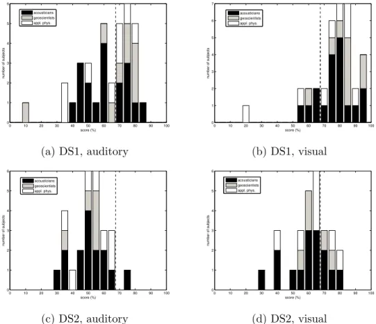
one. All scores are summarized in the histograms of Fig. 4a and b. We 204
suspect the very low scores of two outliers (one per test) to have been caused 205
by a misunderstanding of the intstructions which resulted in the subjects 206
swapping families A and B. 207
For the sake of comparison, we consider the case of entirely random an-208
swers, i.e., the human subject is replaced by an algorithm that generates 209
random yes/no answers, or answers are given by tossing a coin. In this “null 210
hypothesis,” test scores are controlled by the cumulative binomial distribu-211
tion [Press et al., 1992, e.g.]: each signal listened to can be treated as an 212
independent “trial”, with a success probability of 50%. Fig. 4a shows that in 213
the first auditory test about one out of three subjects scored above the 99% 214
confidence level as defined through the cumulative binomial distribution: in 215
other words, the probability that a subject would obtain (at least) such score 216
by giving random answers is less than 1%. It is thus probable that some of 217
the best-scoring subjects have identified a real di↵erence between signals that 218
they classified as belonging to families A and B. Given how we constructed 219
the two families (see “Database” section), it is also reasonable to infer that 220
the auditory clues identified by the subjects are directly related to the e↵ects, 221
on seismic waveforms, of wave propagation through oceanic vs. continental 222
crust. 223
Our data are not numerous enough for the histograms in Fig. 4a,b to 224
clearly suggest specific statistical distributions. By visual inspection of Fig. 4a 225
one might speculate that the distribution of auditory test scores is bimodal, 226
with one peak around 50% corresponding to the null hypothesis, and an-227
other peak around 70% reflecting the performance of subjects who did find 228
meaningful clues in the signals. 229
Scores in the visual test (Fig. 4b) were generally quite high, and higher 230
than for the auditory test. This indicates that, at this point, visual analysis 231
of the data might be a more e↵ective way to complete the task of categorizing 232
DS1 data. 233
Auditory and visual display of DS2 (thrust vs. strike-slip faults) 234
Of the subjects who took part in the experiment described in the previous 235
section, 27 (15 acousticians, 7 physicists, 5 geoscientists; 7 women, 20 men) 236
also participated in a second session, involving 40 signals from DS2. Half of 237
the signals were originated from the strike-slip faults, the other half from the 238
thrust faults shown in Fig. 2b. Again, each subject took an auditory and a 239
visual test, with average scores of 52% and 62%, respectively. The results of 240
both auditory and visual tests are illustrated in Fig. 4c,d. 241
Comparison with the null hypothesis shows that the probability of achiev-242
ing (at least) the average score associated with the visual test by selecting 243
the answers randomly was relatively low (<10%); we infer that at least some 244
subjects are likely to have found visual clues in plotted seismograms. Con-245
versely, the probability of achieving (at least) the average score obtained in 246
the auditory test by giving random answers was about 40%. Too high for 247
the average observed score to be considered significant. It might be guessed 248
that the one subject who achieved a score of 75% might have found auditory 249
clues in the signals, but overall the test cannot be considered a success. 250
Constrained categorization with training
25117 subjects (10 acousticians, 4 physicists, 3 geoscientists; 4 women, 13 men), 252
who had already participated in both the constrained-categorization experi-253
ments, accepted to undergo a training session, followed by an auditory test 254
analogous to those described above. The new exercise was conducted on 255
data from DS2, only half of which were employed in our previous experi-256
ments. Data included in the final test had not been listened to in the course 257
of the training session. The goal of this experiment is to determine whether 258
performance in auditory analysis of seismic data can in principle be improved 259
by training: this is determined below by comparison with performance in a 260
similar task before training. It is therefore not strictly necessary to compare 261
the results against those of visual analysis of the same data, and accordingly 262
the visual test was not repeated. 263
Training 264
Subjects were trained [e.g. Thorndike, 1931; Speeth, 1961] by means of a 265
software interface similar to that used in the actual tests. They first listened 266
to three examples of each family, as before the previous test. They were then 267
presented with up to 24 audified signals in the same way as previously. Half 268
of these signals originated from thrust, the other half from strike-slip faults. 269
Half had been listened to during the previous experiment, half were entirely 270
new. The order in which the signals were presented was random. Upon 271
hearing each signal, subjects were asked by our software interface to evaluate 272
whether it belonged to family A or B. After giving an answer, they were 273
immediately notified whether or not it was “correct” (i.e., consistent with 274
our hypothesis), by the on-screen messages “you have identified the right 275
seismological family” (“vous avez identifi´e la bonne famille sismologique”) 276
and “that is not the right seismological family” (“ce n’est pas la bonne famille 277
sismologique”), respectively. If a subject had a perfect score after listening 278
to the first 16 sample signals, the training session would end. 279
Auditory display of DS2 after training 280
After a brief pause, all subjects who undertook the training session stayed 281
for a final test. 36 signals were randomly picked from DS2. Half of the picked 282
signals had to be from thrust, half from strike-slip faults. Half had to belong 283
to the pool of signals listened to in the test of section “Auditory and visual 284
display of DS2”. 285
The histogram in Fig. 5 shows that scores are generally higher now than 286
when categorizing signals from DS2 before training (Fig. 4c). Only 4 out of 287
17 subjects did not improve their score at all. In the null hypothesis, with 288
36 trials, the probability of achieving a score of at least 69.4% (24 correct 289
answers out of 36) is about 1%: 6 out of 17 subjects scored 70% or more, and 290
we infer that at least some of those 6 learned to recognize relevant auditory 291
clues in the data. Albeit small, these figures appear more significant if one 292
considers that only one brief training session was undertaken. 293
Identifying audio features relevant to
catego-294rization
295At the end of a test, the subject was asked to briefly explain the criteria 296
followed to categorize the signals, via the on-screen message: “according to 297
what criteria have you associated family A and B to the signals?” (“sur 298
quel(s) crit`ere(s) avez vous attribu´e la famille A ou B aux signaux ?”). The 299
subject could answer by typing some comments through our software inter-300
face. 301
Given the difficulty of an exhaustive semantic study of the resulting data 302
[Pat´e et al., 2017], we only give here a preliminary, simplistic analysis of a 303
subset of the recorded comments. Our goal in this endeavour is to identify 304
some of the auditory clues that lead subjects to make their choices. We focus 305
on the subjects whose scores were highest, as the criteria that guided them 306
are probably related to the geophysical parameters that defined our families 307
of signals. 308
Comments on DS1
309We first analyze the comments made by 5 subjects (2 acousticians, 2 geosci-310
entists, and one physicist) who all achieved scores 80% in discriminating
311
audified seismograms corresponding to oceanic vs. continental paths (DS1). 312
Table 2 shows a number of reoccurring suggested clues, namely: the pres-313
ence of what the subjects identify as “background noise,” and its timbre; 314
the duration of what is considered by the subjects to be meaningful signal; 315
the identification of “echos” in the signal. These features can in principle be 316
associated to quantities calculated by seismic data analysis. 317
First of all, it is relatively easy to identify the onset of an earthquake 318
recording on a seismogram (i.e., the P -wave arrival), and it is then reasonable 319
to define as background noise the signal recorded before such arrival. In all 320
our recordings, the first 500 samples clearly precede the arrival of the main 321
signal and we accordingly identify them as noise. We define the beginning 322
of the seismic signal as the first recorded sample whose amplitude is at least 323
three times larger than the largest amplitude found within the 500 noise 324
samples. Let nS denote its index. The signal-to-noise ratio (SNR) in decibels
325
can then be estimated, based on the mean amplitudes of signal and noise, by 326 the formula 327 SNR = 10 log10 "PN i=nSs 2[i] P500 i=1s2[i] # , (1)
where s[i] is the amplitude of the i-th sample, in a recording that consists of N 328
samples total. We compute the SNR of all signals in DS1, and find (Fig. 6a) 329
that continental paths tend to be associated with higher SNR values than 330
oceanic paths. This statistical result is in qualitative agreement with the 331
subjects comments. 332
We evaluate the “timbre” of background noise by taking the Fourier trans-333
form of the first 500 samples only. Fig. 6b shows the distribution of frequency 334
values corresponding to the highest spectral peak in the resulting Fourier 335
spectrum: whether the terrain traversed by the propagating seismic wave is 336
oceanic or continental does not appear to a↵ect significantly the frequency 337
content of noise. 338
We next attempt to quantify the duration of meaningful seismic signal 339
which the subjects believe to have recognized in their listening experiences: 340
after the main, high-amplitude interval that includes body- and surface-wave 341
arrivals, the peak amplitude of all our signals decreases until it becomes as 342
low as the peak amplitude of background noise. For each seismogram, we find 343
the latest sample whose peak amplitude is as large as 10% of its maximum 344
recorded value for that seismogram; we then measure the length of the time 345
interval that separates it from the maximum-amplitude sample, and define 346
it as the duration of seismologically meaningful signal. Fig. 6c shows how 347
such values are distributed for signals associated with oceanic vs. continental 348
propagation paths, and indicates that oceanic signals are, according to our 349
definition, longer than continental ones. 350
Finally, echos can be identified by visual analysis of a seismogram’s en-351
evelope. We calculate the envelopes of all our audified seismograms, and take 352
the averages of all oceanic-path and all continental-path envelopes. In anal-353
ogy with Pat´e et al. [2017], the envelope is defined as suggested by D’Orazio 354
et al. [2011]: starting with i coinciding with the index of the last sample in 355
a signal, if sample i 1 exceeds sample i, then the value of sample i 1
356
is saved as the i-th entry of the envelope; the procedure is iterated for the 357
preceding sample, until the entire trace is processed [D’Orazio et al., 2011, 358
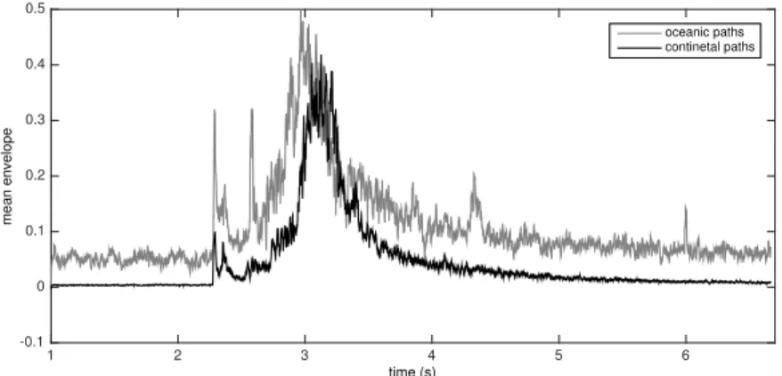
figure 5]. The results of this exercise, illustrated in Fig. 7, show that (i) the 359
amplitude of oceanic-path signal is generally larger than that of continental-360
path signal; (ii) the oceanic-path signal is characterized by a number of 361
high-amplitude peaks that are not visible in the continental-path one; (iii) 362
the large-amplitude portion of the signal lasts longer in oceanic-path than 363
continental-path signal. While the standard deviations of both envelopes 364
are not shown in Fig. 7 in the interest of readability, these inferences are 365
confirmed even if the standard deviation is taken into account. We note 366
that the standard deviation of the oceanic-path envelope is larger than the 367
continental-path one. Observation (ii) reflects several comments made by the 368
subjects (Table 2). 369
Comments on DS2
370The four subjects who achieved the highest scores (> 55%) without training 371
are combined with the four who achieved the highest scores (> 72%) after 372
training, resulting in a group of eight subjects whose verbal comments are 373
summarized in table 3. The group includes three geoscientists, three acous-374
ticians, and two physicists. Two of the subjects in this group were also in 375
the group discussed in the previous section. 376
Table 3 shows that, despite some contradictory comments, most subjects 377
find strike-slip-fault signals to be characterized by a relatively weak “first 378
arrival” followed by a high-energy coda, while on the contrary they associate 379
thrust events with a strong first arrival followed by a weaker coda. This seems 380
to be consistent with the average envelopes of Fig. 8, where (i) the initial 381
peak is clearly identifiable for both families and is roughly twice as high 382
in the inverse-fault case, with respect to the strike-slip-fault one, while (ii) 383
the later inverse-fault signal is of higher amplitude than its strike-slip-fault 384
counterpart, with a ⇠20% di↵erence in their main peaks. If the envelopes’
385
standard deviations (not shown in Fig. 8 for clarity) are taken into account, 386
however, this observation cannot be confirmed; more tests, with a broader 387
data set, need to be conducted to come to a definitive conclusion. 388
Influence of subjects’ background on the
re-389sults
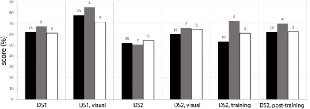
390Fig. 9 shows that test scores are not strongly a↵ected by the background of 391
subjects. The average score achieved by geoscientists is always (except for 392
the auditory categorization of DS2) slightly higher than that of the other two 393
groups, but the subjects are not numerous enough for this small di↵erence 394
to be considered significant. 395
On the other hand, our analysis of the subjects’ recorded descriptions 396
of their categorization strategy shows that acousticians have used about 20 397
more words than both other groups to qualify sounds. We interpret this result 398
as a natural consequence of the acousticians’ specific expertise in describing 399
sounds, while geoscientists and physicists usually represent their data only 400
visually. This speculation is confirmed by the study of Pat´e et al. [2017], 401
who conducted a thorough, quantitative analysis of verbal data collected in 402
a similar experiment (also involving audified seismic data, and subjects with 403
similar backgrounds). 404
Discussion
405Conclusions
406In our experiments, listeners were exposed to two audified seismic data sets, 407
each characterized by a single, binary control factor: the orientation of the 408
fault (strike-slip or thrust) in one case, the nature of the tectonic plate 409
through which the recorded signal had traveled prior to recording (oceanic 410
or continental) in the other. They were then asked to split each data set into 411
two categories, based on examples of signals associated with di↵erent values 412
of the control factor. Purely auditory tests were compared with similar tests, 413
where data were displayed visually rather than acoustically. Overall, listen-414
ers were able to categorize data based on audition alone. Their performance 415
in visual tests was better, but performance in auditory categorization was 416
significantly improved by a brief training session. 417
Asked to comment on the criteria they had chosen to categorize, listeners 418
most often pointed to perception-based physical features that can be summa-419
rized as: signal-to-noise ratio (SNR); the duration of what they interpreted 420
to be meaningful signal as opposed to background noise; the frequency con-421
tent of background noise; the relative amplitude of first seismic “arrivals” 422
with respect to coda. At least two of these features (SNR and meaningful 423
signal duration) do correspond to quantitative parameters that we have been 424
able to define and calculate by simple data processing; we show in Fig. 6a,c 425
that those parameters are di↵erently distributed depending on the value of 426
the relevant control parameter. 427
In summary, human listeners are able to identify geophysically relevant 428
features of audified seismic data, and can be trained to improve their per-429
formance at such tasks. We cannot yet predict the extent to which training 430
can refine our skills at interpreting the data by listening, but we surmise 431
that auditory display can be useful to a variety of endeavors in seismic data 432
analysis. 433
Outlook
434While the resolution and pattern recognition capabilities of the human au-435
ditory system are generally well known [e.g., Hartmann, 1999; Wang and 436
Brown, 2006a], the seismology community does not entirely appreciate the 437
potential of auditory display as a tool for seismic data analysis. A case in 438
point is the interesting work of Moni et al. [2012] and Moni et al. [2013], 439
where an algorithm designed to mimic the human auditory system (in the 440
words of the authors, “to solve the ‘cocktail party problem,’ i.e., separating 441
individual speakers in a room with multiple speakers”) was successfully ap-442
plied to the problem of identifying di↵erent simultaneous microseisms, and 443
yet no attempt was made to use the human auditory system itself, simply 444
listening to the audified data. 445
Besides the benefits derived from exploiting the natural skills of our audi-446
tory system, audification typically involves the acceleration of a seismic signal 447
by a factor between ⇠ 102 and ⇠ 103, depending on the frequency content
448
of the original data, which means that an entire day of seismic recording can 449
be listened to in a few minutes with little or no loss of information. Being 450
able to rapidly analyze large sets of data is important, as seismologists are 451
faced today with large and rapidly growing databases. For instance, precisely 452
locating the epicenters of seismic aftershocks requires solving an enormous 453
number of inverse problems [e.g., Valoroso et al., 2013]. This cannot be en-454
tirely automated if reliable results are to be otbained. All signals recorded by 455
a seismic network can however be listened to simultaneously, by the princi-456
ples of sound spatialization [e.g. Peters et al., 2011], in an anechoic chamber 457
equipped with a dense speaker network or, more simply, binaurally. The 458
human auditory system is naturally equipped to locate the source of a sound 459
[e.g. Hartmann, 1999; Wang and Brown, 2006b], and, through this setup, it 460
is reasonable to hypothesize that one might be able to learn to roughly but 461
quickly locate earthquake epicenters (global, regional or local) by listening 462
to sets of audified seismograms. This approach would involve some impor-463
tant approximations (neglect of dispersion and of Earth lateral heterogeneity 464
e↵ects, etc.), but could be very practical because of its speed and simplicity. 465
The auditory properties of audified seismograms have also been shown to 466
be indicative of several specific seismic processes, including mainshock/aftershock 467
sequences, earthquake swarms that accompany volcanic eruptions, or deep 468
non-volcanic tremors [Kilb et al., 2012; Peng et al., 2012]. Audification is 469
likely to find other potentially important applications in seismology, wher-470
ever large datasets are to be investigated, and unknown/unexpected patterns 471
recognized. Examples include the analysis of the Earth’s seismic background 472
signal [e.g. Boschi and Weemstra, 2015] with implications for monitoring of 473
natural hazards [e.g. Wegler and Sens-Schonfelder , 2007; Brenguier et al., 474
2008], and the problem of determining the evolution of a seismic rupture 475
in space and time from the analysis of seismic data [e.g., Ide, 2007; Mai 476
et al., 2016]. The study of large sets of audified data can further benefit 477
from the possibilities o↵ered by crowd-sourcing platforms: if the sounds are 478
short and meaningful enough, if the listeners’ task is simple enough, and if 479
the data set is correctly distributed among listeners (each sound is given to 480
at least one listener, some are given to several listeners for verification and 481
variability assessment), then a large data set can be e↵ectively explored by 482
the “collaborative” work of a number of listeners. 483
Data and resources
484The image and audio files that were presented to subjects in all the experi-485
ments described here are available online at http://hestia.lgs.jussieu.fr/ boschil/downloads.html. 486
The Global Centroid Moment Tensor Project database was searched using 487
www.globalcmt.org/CMTsearch.html (last accessed September 2016). 488
The IRIS database was searched via the Wilber interface at http://ds.iris.edu/wilber3/find event 489
(last accessed September 2016). 490
Figs. 1 and 2 were made using the Generic Mapping Tools version 5.2.1 491
[Wessel and Smith, 1991, www.soest.hawaii.edu/gmt]. 492
Acknowledgements
493We acknowledge financial support from INSU-CNRS, and from the European 494
Union’s Horizon 2020 research and innovation programme under the Marie 495
Sklodowska-Curie grant agreement No. 641943 (ITN WAVES). Dani`ele Dubois 496
and Piero Poli have contributed to our work through many fruitful discus-497
sions. Zhigang Peng, Debi Kilb and one anonymous reviewer provided careful 498
reviews of our original manuscript. We are grateful to the volunteers who 499
kindly accepted to take our tests. 500
References
501Boschi, L., and C. Weemstra, Stationary-phase integrals in
502
the cross-correlation of ambient noise, Rev. Geophys., 53,
503
doi:10.1002/2014RG000,455, 2015. 504
Brenguier, F., N. M. Shapiro, M. Campillo, V. Ferrazzini, Z. Duputel, 505
O. Coutant, and A. Nercessian, Towards forecasting volcanic eruptions 506
using seismic noise, Nat. Geosci., 1, 126–130, 2008. 507
Cowen, R., Sound bytes, Scientific American, 312, 4447, 2015. 508
Dombois, F., and G. Eckel, Audification, in The Sonification Handbook, 509
edited by T. Hermann, A. Hunt, and J. G. Neuho↵, pp. 301–324, Berlin: 510
Logos Publishing House, 2011. 511
D’Orazio, D., S. De Cesaris, and M. Garai, A comparison of methods to 512
compute the e↵ective duration of the autocorrelation function and an al-513
ternative proposal, J. Acoust. Soc. Am., 130, 19541961, 2011. 514
Ekstr¨om, G., M. Nettles, and A. M. Dziewo´nski, The global CMT project
515
2004-2010: Centroid-moment tensors for 13,017 earthquakes, Phys. Earth 516
Planet. Inter., 200-201, 1–9, 2012. doi:10.1016/j.pepi.2012.04.002 , 2012. 517
Frantti, G. E., and L. A. Leverault, Auditory discrimination of seismic signals 518
from earthquakes and explosions, Bull. Seism. Soc. Am., 55, 1–25, 1965. 519
Gaillard, P., Laissez-nous trier ! TCL-LabX et les tˆaches de cat´egorisation 520
libre de sons, in Le Sentir et le Dire, edited by D. Dubois, pp. 189–210, 521
L’harmattan, Paris, France, 2009. 522
Hartmann, W. M., How we localize sound, Phys. Today, 11, 24–29, 1999. 523
Holtzman, B., J. Candler, M. Turk, and D. Peter, Seismic sound lab: Sights, 524
sounds and perception of the earth as an acoustic space, in Sound, Music, 525
and Motion, edited by M. Aramaki, O. Derrien, R. Kronland-Martinet, 526
and S. Ystad, pp. 161–174, Springer International Publishing, 2014. 527
Ide, S., Slip inversion, in Treatise of Geophysics, Vol. 4, edited by 528
H. Kanamori, pp. 193–223, Elsevier, Amsterdam, 2007. 529
Kennett, B. L. N., and T. Furumura, High-frequency P o/So guided waves 530
in the oceanic lithosphere: I-long distance propagation, Geophys. J. Int., 531
195, 1862–1877, doi: 10.1093/gji/ggt344, 2013. 532
Kennett, B. L. N., T. Furumura, and Y. Zhao, High-frequency P o/So guided 533
waves in the oceanic lithosphere: II-heterogeneity and attenuation, Geo-534
phys. J. Int., 199, 614–630, doi: 10.1093/gji/ggu286, 2014. 535
Kilb, D., Z. Peng, D. Simpson, A. Michael, and M. Fisher, Listen, 536
watch, learn: SeisSound video products, Seismol. Res. Lett., 83, 281–286, 537
doi:10.1785/gssrl.83.2.281, 2012. 538
Mai, P. M., et al., The earthquake-source inversion validation (SIV) project, 539
Seism. Res. Lett., 87, 690–708, doi:10.1785/0220150,231, 2016. 540
Moni, A., , C. J. Bean, I. Lokmer, and S. Rickard, Source sep-541
aration on seismic data, IEEE Signal Process Mag., 29, 16–28, 542
doi:10.1109/MSP.2012.2184,229, 2012. 543
Moni, A., D. Craig, and C. J. Bean, Separation and location of microseism 544
sources, Geophys. Res. Lett., 40, 3118–3122, doi:10.1002/grl.50,566, 2013. 545
Pat´e, A., L. Boschi, J. L. le Carrou, and B. Holtzman, Categorization of 546
seismic sources by auditory display: a blind test, International Journal 547
of Human-Computer Studies, 85, 57–67, doi:10.1016/j.ijhcs.2015.08.002, 548
2016. 549
Pat´e, A., L. Boschi, D. Dubois, B. Holtzman, and J. L. le Carrou, Auditory 550
display of seismic data: Expert categorization and verbal description as 551
heuristics for geoscience, J. Acoust. Soc. Am., accepted, 2017. 552
Peng, Z., C. Aiken, D. Kilb, D. Shelly, and B. Enescu, Listening to the 2011 553
magnitude 9.0 Tohoku-Oku, Japan earthquake, Seismol. Res. Lett., 83, 554
287–293, doi:10.1785/gssrl.83.2.287, 2012. 555
Peters, N., G. Marentakis, and S. McAdams, Current technologies and com-556
positional practices for spatialization: A qualitative and quantitative anal-557
ysis, Computer Music Journal, 35, 10–27, 2011. 558
Press, W. H., S. A. Teukolsky, W. T. Vetterling, and B. P. Flannery, Numer-559
ical Recipes in Fortran 77, Cambridge University Press, 1992. 560
Speeth, S. D., Seismometer sounds, J. Acoust. Soc. Am., 33, 909–916, 561
doi:10.1121/1.1908,843, 1961. 562
Tang, Y., Data sonification with the seismic signature of ocean surf, The 563
Leading Edge, 33, doi:10.1190/tle33101,128.1, 2014. 564
Thorndike, E. L., Human Learning, Century, New York, 1931. 565
Valoroso, L., L. Chiaraluce, D. Piccinini, R. D. Stefano, D. Scha↵, and 566
F. Waldhauser, Radiography of a normal fault system by 64,000 high-567
precision earthquake locations: The 2009L’Aquila (central Italy) case 568
study, J. Geophys. Res., 118, 1156–1176 doi:10.1002/jgrb.50,130, 2013. 569
Volmar, A., Listening to the Cold War: The Nuclear Test Ban negotiations, 570
seismology, and psychoacoustics, 1958-1963, Osiris, 28, 80–102, 2013. 571
Wang, D., and G. J. Brown, Fundamentals of computational auditory scene 572
analysis, in Computational Auditory Scene Analysis, edited by D. Wang 573
and G. J. Brown, pp. 1–44, Wiley & Sons, Hoboken, N. J., 2006a. 574
Wang, D., and G. J. Brown, Computational Auditory Scene Analysis, Wiley 575
& Sons, Hoboken, N. J., 2006b. 576
Wegler, U., and C. Sens-Schonfelder, Fault zone monitoring with passive 577
image interferometry, Geophys. J. Int., 168, 1029–1033, 2007. 578
Wessel, P., and W. H. F. Smith, Free software helps map and display data, 579
EOS Trans. Am. Geophys. Union, 72, 445–446, 1991. 580
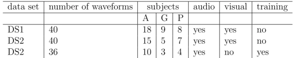
Table 1: Summary of listening experiments.
data set number of waveforms subjects audio visual training
A G P
DS1 40 18 9 8 yes yes no
DS2 40 15 5 7 yes yes no
DS2 36 10 3 4 yes no yes
The first two columns to the left indicate how many signals from which data set were presented to the subjects. The letters A, G and P stand for “acous-ticians,” “geoscientists” and “physicists,” respectively; “audio” and “visual” indicate which type(s) of data were provided to the subjects; “training” refers to whether subjects were trained before taking the test.
Table 2: Listeners’ comments on DS1.
Family A (oceanic paths) Family B (continental paths) second shock very close to the first echo of the first impact’s sound
with an echo / rebound small rebounds
a lot of background noise little background noise high-pitched background noise low-pitched background noise
background noise shorter and duller sound
longer signal sharper and shorter
rising perceived frequency faster arrival
buzz or intense reverberation after the explosion
Summary of written, verbal explanations given by 5 subjects (scoring 80%)
concerning their auditory cateogorization of DS1. All text was originally in French and has been translated into English as literally as possible.
Table 3: Listeners’ comments on DS2.
Family A (strike-slip events) Family B (thrust events) first shock weaker than second one louder low frequencies
wave of rising frequency louder than the first heard shock first shock louder than the second one after the detonation, sound decays more slowly first shock louder than the wave
faster attack and decay more powerful and present sound significant intensity even after a long time sound decays quickly after the detonation
lower-frequency shock slower decay
duller signal higher frequencies
Summary of written, verbal explanations given by 8 subjects (scoring 80%)
for the auditory cateogorization of DS2 before (4 subjects scoring > 55%) and after training (4 subjects scoring > 72%). Again, the original French text was translated into English.
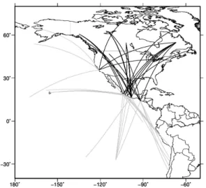
Figure 1: Surface projections of ray paths associated with audified data set DS1. DS1 consists of recordings of events occurring along the west coast
of Mexico, made at stations at epicentral distances of ⇠4000 to 6000 km;
recordings made at north American stations correspond to ray paths only traversing continental terrain (black lines), while stations along the Pacific coast or on ocean islands result in purely oceanic paths (grey lines).
(a) (b)
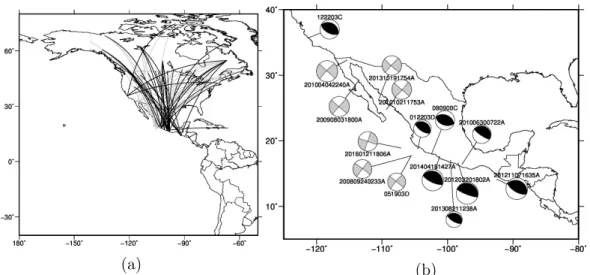
Figure 2: (a) Same as Fig. 1, but for data set DS2, which only includes recordings made at stations within the north American continent, of either strike-slip (grey ray path curves) or thrust (black) events. Their epicenters and focal mechanisms [Ekstr¨om et al., 2012] are shown in (b) using the same color code.
(a) (b)
(c) (d)
(e) (f)
(g) (h)
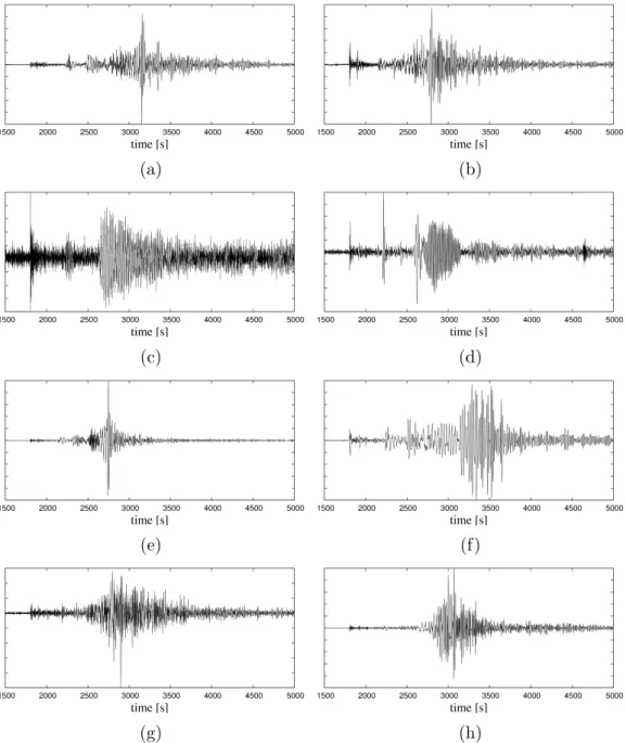
Figure 3: Examples of seismograms used in our study. (a) and (b): DS1, continental paths. (c) and (d) DS1: oceanic paths. (e) and (f): DS2, thrust faults. (g) and (h) DS2, strike-slip faults. The vertical axis is not labeled as we systematically normalize all seismograms (both visual and audio). In our visualization experiments, the horizontal axis was less exaggerated and the time span much longer, so that in principle the exact same information was provided to subjects in visualization and listening tests. The images files used in experiments are available online (see “Data and resources” section).
0 10 20 30 40 50 60 70 80 90 100 0 1 2 3 4 5 6 score (%) number of subjects acousticians geoscientists appl. phys. (a) DS1, auditory 0 10 20 30 40 50 60 70 80 90 100 0 1 2 3 4 5 6 7 score (%) number of subjects acousticians geoscientists appl. phys. (b) DS1, visual 0 10 20 30 40 50 60 70 80 90 100 0 1 2 3 4 5 6 score (%) number of subjects acousticians geoscientists appl. phys. (c) DS2, auditory 0 10 20 30 40 50 60 70 80 90 100 0 1 2 3 4 5 6 score (%) number of subjects acousticians geoscientists appl. phys. (d) DS2, visual
Figure 4: These histograms summarize the results of the constrained catego-rization experiments conducted before training on audified seismograms from data sets DS1 (panels (a) and (b)) and DS2 ((c) and (d)). Scores achieved in auditory tests are shown in panels (a) and (c); scores achieved in visual tests are shown in (b) and (d). The vertical dashed line marks the “99% confidence level,” i.e. the probability of achieving at least that score by cat-egorizing the signal at random is less than 1%. Colors correspond to the di↵erent background of subjects, as explained in the inset.
0 10 20 30 40 50 60 70 80 90 100 0 0.5 1 1.5 2 2.5 3 3.5 4 score (%) number of subjects acousticians geoscientists appl. phys.
Figure 5: Histogram summarizing the results of the constrained categoriza-tion experiment conducted (on DS2) after training. The vertical dotted line, corresponding to a score of 69.4%, marks the 99% confidence level; all scores in the 67.5%-to-72.5% bin actually fall to its right.
(a) 10 20 30 40 50 si g n a l− to − n o ise ra ti o Family B Family A (b) 150 200 250 300 350 400 fre q u e n cy (H z) Family B Family A (c) 2 3 4 5 si g n a l d u ra ti o n (s) Family B Family A
Figure 6: Distributions, shown as box-plots, of three physical parameters, corresponding to properties of the signal that subjects tend to describe as important: (a) SNR; (b) dominant frequency of background noise; (c) dura-tion of meaningful signal. For each parameter, the distribudura-tions of parameter values for oceanic-path (“Family A) and continental-path (“Family B) signal are shown separately. Distributions are summarized by their median (thick grey segments), first and third quartiles (upper and lower sides of boxes), and minimum and maximum values (endpoints of dashed lines). Values that we neglect as outliers (their absolute value is more than 1.5 times the in-terquartile distance) are denoted by grey crosses.
time (s) 1 2 3 4 5 6 mean envelope -0.1 0 0.1 0.2 0.3 0.4 0.5 oceanic paths continetal paths
Figure 7: Signal envelope averaged over all DS1 audified seismograms corre-sponding to continental (black line) vs. oceanic (grey) paths.
time (s) 1 2 3 4 5 6 mean envelope -0.1 0 0.1 0.2 0.3 0.4 0.5 0.6 strike-slip thrust
Figure 8: Same as Fig. 7, but envelopes are averaged over all DS2 signals originated from thrust (black line) vs. strike-slip (grey) events.
Figure 9: Average scores by test (left to right, as indicated under each bar) and by subjects’ background group. Black, grey and white bars are associated with acousticians, geoscientists and physicists, respectively. The number of subjects participating to a test is shown above the corresponding bar. The label “post-training” refers to the auditory test of DS2 conducted after the training session; “training” refers to answers that were given during the aforementioned training session.