HAL Id: hal-01087388
https://hal.archives-ouvertes.fr/hal-01087388
Submitted on 26 Nov 2014HAL is a multi-disciplinary open access archive for the deposit and dissemination of sci-entific research documents, whether they are pub-lished or not. The documents may come from teaching and research institutions in France or abroad, or from public or private research centers.
L’archive ouverte pluridisciplinaire HAL, est destinée au dépôt et à la diffusion de documents scientifiques de niveau recherche, publiés ou non, émanant des établissements d’enseignement et de recherche français ou étrangers, des laboratoires publics ou privés.
Incorporation of diet information derived from Bayesian
stable isotope mixing models into mass-balanced marine
ecosystem models: A case study from the
Marennes-Oléron Estuary, France
Stephen Pacella, Benoit Lebreton, Pierre Richard, Donald Phillips, Theodore
Dewitt, Nathalie Niquil
To cite this version:
Stephen Pacella, Benoit Lebreton, Pierre Richard, Donald Phillips, Theodore Dewitt, et al.. Incor-poration of diet information derived from Bayesian stable isotope mixing models into mass-balanced marine ecosystem models: A case study from the Marennes-Oléron Estuary, France. Ecological Mod-elling, Elsevier, 2013, 267, pp.127 - 137. �10.1016/j.ecolmodel.2013.07.018�. �hal-01087388�
Incorporation of diet information derived from Bayesian stable isotope mixing models into mass-balanced marine ecosystem models: A case study from the Marennes-Oléron Estuary, France
Stephen PACELLA1,2*, Benoit LEBRETON3, Pierre RICHARD3, Donald PHILLIPS2,
Theodore DEWITT2, Nathalie NIQUIL3
1College of Earth, Ocean, and Atmospheric Sciences, Oregon State University, 104
Wilkinson Hall, Corvallis, OR, 97331, USA
2Western Ecology Division, Office of Research and Development, National Health and
Environmental Effects Research Laboratory, United States Environmental Protection
Agency, 200 SW 35th Street, Corvallis, OR, 97333
3Université de la Rochelle-CNRS, UMR 6250, Littoral Environnement et Sociétés
(LIENSs), 2 rue Olympe de Gouges, F-17000 La Rochelle, France
ABSTRACT
We investigated the use of output from Bayesian stable isotope mixing models as constraints for a linear inverse food web model of a temperate intertidal seagrass system in the Marennes-Oléron Bay, France. Linear inverse modeling (LIM) is a technique that estimates a complete network of flows in an under-determined system using a
combination of site-specific data and relevant literature data. This estimation of complete flow networks of food webs in marine ecosystems is becoming more recognized for its utility in understanding ecosystem functioning. However, diets and consumption rates of organisms are often difficult or impossible to accurately and reliably measure in the field, resulting in a large amount of uncertainty in the magnitude of consumption flows and resource partitioning in ecosystems. In order to address this issue, this study utilized
stable isotope data to help aid in estimating these unknown flows. δ13C and δ15N isotope
data of consumers and producers in the Marennes-Oléron seagrass system was used in Bayesian mixing models. The output of these mixing models was then translated as inequality constraints (minimum and maximum of relative diet contributions) into an inverse analysis model of the seagrass ecosystem. We hypothesized that incorporating the diet information gained from the stable isotope mixing models would result in a more constrained food web model. In order to test this, two inverse food web models were built to track the flow of carbon through the seagrass food web on an annual basis, with
units of mg C m-2 d-1. The first model (Traditional LIM) included all available data, with
the exception of the diet constraints formed from the stable isotope mixing models. The second model (Isotope LIM) was identical to the Traditional LIM, but included the SIAR diet constraints. Both models were identical in structure, and intended to model the same
Marennes-Oléron intertidal seagrass bed. Each model consisted of 27 compartments (24 living, 3 detrital) and 175 flows. Comparisons between the outputs of the models showed the addition of the SIAR-derived isotopic diet constraints further constrained the solution range of all food web flows on average by 26%. Flows that were directly affected by an isotopic diet constraint were 45% further constrained on average. These results
confirmed our hypothesis that incorporation of the isotope information would result in a more constrained food web model, and demonstrated the benefit of utilizing multi-tracer stable isotope information in ecosystem models.
Keywords: Ecological model; Stable isotope; Inverse analysis; Food web; Seagrass
1. INTRODUCTION
Current ecological questions are often complex in nature, requiring a holistic perspective in order to adequately address the multitude of variables and relationships. There is thus an ever-increasing pressure on ecologists to address these questions at the ecosystem scale. Quantitative food web models, representing partial or whole ecosystem flux networks, are a promising methodology to address ecological questions (Christian et al., 2009; Leslie and McLeod, 2007). These models are able to simultaneously explore effects of environmental changes on ecosystem structure and function, as well as emergent properties such as system dependencies, recycling, and efficiencies (Niquil et al., 2012). Banašek-Richter et al. (2004) showed that ecosystem descriptors based on quantified systems models are more accurate than their qualitative counterparts. Estimation of complete flux networks of food webs in marine ecosystems is recognized
for its utility to understand ecosystem functioning (Niquil et al., 2012). However, many components of ecosystem models are understood conceptually, but difficult or impossible to measure in the field, and therefore must be estimated (Niquil et al., 1998; van Oevelen et al., 2010; Vezina and Platt, 1988).
Inverse analysis is a powerful quantitative modeling method for estimating unmeasured components in ecosystem structures (Legendre and Niquil, 2012) and has been widely used for this reason in food web modeling (Breed et al., 2004; Daniels et al., 2006; Degré et al., 2006; Donali et al., 1999; Eldridge et al., 2005; Eldridge and Jackson, 1993; Grami et al., 2008; 2011; Jackson and Eldridge, 1992; Kones et al., 2009;
Leguerrier et al., 2007; 2003; Niquil et al., 1998; 2006). It has become commonly referred to as Linear Inverse Modeling (LIM). Similarly to ECOPATH with ECOSIM (Christensen and Pauly, 1992; Pauly, 2000; Walters et al., 1997), LIM produces a static, mass-balanced, temporally integrated snapshot of the complete food web. Recent methodological advances have resulted in moving from models being solved with a single objective function (frequently a minimization function, (Vezina and Platt, 1988); Legendre and Niquil, 2012), to utilizing stochastic Markov Chain Monte Carlo methods to produce probability distributions of model results (LIM-MCMC) (Kones et al., 2009; 2006; Van den Meersche et al., 2009; van Oevelen et al., 2010). This technique avoids underestimates in both the size and complexity of the modeled food web as a result of the parsimony principle (Johnson et al., 2009; Kones et al., 2006). A more thorough review on the subject is covered by Niquil et al. (2012). Few applied studies have made use of recent methodological advances in this field, despite the relevance to informing
conservation and environmental management decisions (Christian et al., 2009);Jorgensen 2007).
Stable isotopes are commonly used to study trophodynamics in ecosystems. Stable isotope analyses allow determination of food sources actually assimilated in the tissues of consumers over time, properly reflecting their trophodynamics depending on food source availability (Fry, 2006). Consumption rates are often difficult or impossible to accurately measure in the field, especially for smaller organisms, resulting in a large uncertainty in the magnitude of consumption flows and trophic resource partitioning in ecosystem models. Stable isotope data can be utilized to estimate these unmeasured flows (Navarro et al., 2011; van Oevelen et al., 2010). While the use of stable isotopes in diet studies has become standard practice (Moore and Semmens, 2008; Post, 2002), the integration of stable isotope data with whole food web network models has not been utilized frequently (Baeta et al., 2011; Navarro et al., 2011). The merits of this technique have been discussed recently in the literature (Navarro et al., 2011; van Oevelen et al., 2010).
Until now, only one stable isotopic marker (δ13C or δ15N) at a time has been
incorporated into inverse analysis models (Eldridge et al., 2005; Jackson and Eldridge, 1992; Oevelen et al., 2010; van Oevelen et al., 2006). Using two or more isotopic markers significantly increases model structure complexity and greatly increases model run time. This problem is compounded in situations where Monte Carlo methods are used to run the inverse analysis thousands of times (Kones et al., 2009; Niquil et al., 2012; van Oevelen et al., 2010). This has significant implications when attempting to
add stable isotope information into food web models solved using the new Linear Inverse Model-Markov Chain Monte Carlo techniques (Kones et al., 2009; Niquil et al., 2012).
Therefore, the goal of this study was to find a way to incorporate information
from multiple stable isotope elements (i.e., 13C, 15N, etc.) into food web models using the
LIM-MCMC technique, with minimum added complexity. In order to do this, we used
the R package SIAR (Parnell et al., 2010) to analyze Bayesian mixing models using δ13C
and δ15N data to estimate food source distributions of the compartments in an inverse
food web model of an intertidal seagrass bed. This information was then integrated into the LIM-MCMC food web model. Results of this model were compared with a
corresponding model of the same system that excluded the isotope information obtained with the SIAR mixing models. We hypothesized that incorporating the food source information gained from the stable isotope information into the LIM-MCMC model would result in a significantly more constrained food web model, with reduced uncertainty associated with each flow.
2. METHODS
2.1 Marennes-Oléron Bay study site and model data
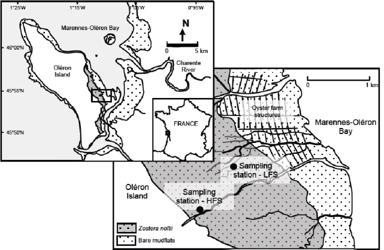
The seagrass system studied was an intertial Zostera noltii meadow located in Marennes-Oléron Bay, on the Atlantic coast of France (45°54’N, 1°12’W) (Figure 1). This is a semi-enclosed, macrotidal bay, which receives freshwater inputs from the
Charente River (15-500 m3 s-1) (Ravail-Legrand et al., 1988). The seagrass bed studied
Primary producer biomass, benthic consumer biomass, and stable isotope data used in this model were obtained from (Lebreton et al., 2012; 2009). Sampling was conducted at two stations (a high flat station and a low flat station) in 2006 and 2007 (Figure 1) and the results were averaged (Table 1). Each station was a homogeneous area
of 100 m2 parallel to the coastline, about 250 m from the upper and lower limits of the
seagrass bed, respectively. The stations were each broken up into 100 plots of 1 m2 for
sampling. Both sampling sites were exposed at every low tide, with the higher in elevation of the two sites being exposed for 5 hours longer on average (Lebreton et al., 2009). Average emersion times on the seagrass bed were computed for this study using bathymetric data and tidal measurements, and those processes (i.e., phytoplankton production, bird grazing, zooplankton grazing, etc.) affected by the tidal cycle were scaled accordingly in the food web model.
2.2 Linear Inverse Model (LIM-MCMC) formulation
Two inverse food web models were built to track the flow of carbon through the
seagrass food web on an annual basis, with units of mgC m-2 d-1. The first model
(Traditional LIM) included all available data, with the exception of the diet constraints formed from the stable isotope mixing models. The second LIM (Isotope LIM) was identical to the Traditional LIM, but included the SIAR diet constraints. Both models were identical in structure, and intended to model the same Marennes-Oleron intertidal seagrass bed.
First, an a priori topological model was formulated of the food web based on local expert knowledge and previous studies (Leguerrier et al., 2003; 2004), defining the
compartments and all probable connections between them. All macrofaunal species sampled in the system were included which had a biomass of at least 0.05 g ash-free dry
weight m-2. This biomass threshold value resulted in 96.5% of the total measured
biomass during sampling being included in the inverse food web model. The benthic and pelagic fauna of the system were parsed into compartments based on similarity of
species-specific characteristics such as taxonomy, habitat, known feeding habits, known
predators, and stable isotope (δ13C and δ15N) values. Priority was placed on aggregating
species into the compartments in such a way so as to balance between maintaining the true trophic complexity of the ecosystem versus the need to keep the model simple enough that solutions could be produced in a timely manner. As the complexity of the model scales exponentially with the number of compartments, some aggregation was necessary. However, loss in precision of stable isotope data due to aggregation of species with dissimilar signatures was considered to be undesirable for the mixing models, and was therefore avoided. Previous studies found that a priori model aggregation at low trophic levels has a greater effect on inverse model results than does aggregation of higher trophic levels (Johnson et al., 2009). In light of these results, primary producers, bacteria, and non-living carbon pools (e.g., dissolved organic carbon) were each given their own compartment. The resulting a priori food web model consisted of 26
compartments (23 living, 3 detrital) (Table 1) and 175 flows among compartments (Table 2).
The Traditional LIM and Isotope LIM were run using a Matlab routine that was a translation of the R packages limSolve and xsample (Kones et al., 2009; Van den
Monte Carlo (MCMC) algorithm to sample the LIM solution space using random jumps of a user-defined length. A “mirror” algorithm within the Matlab program creates a set of hyperplanes that form a convex solution space based on the equality and inequality constraints, out of which the sampling procedure cannot exit (Van den Meersche et al., 2009). These hyperplanes act as mirrors, which the random jumps are reflected by, and that ensure the samples are always taken from within the LIM feasible solution space. This procedure reduces the number of iterations required to fully characterize the solution space when compared with a solution procedure whose searching is not constrained to within the feasible solution space, as all samples of the mirror algorithm procedure are feasible solutions. Adequate sampling of the solution space and convergence was ensured through visual inspection of the sampling and results for each flow of the food web model. Note that the models were solved using the LIM-MCMC technique as described above, but will be referred to as the Traditional LIM and Isotope LIM for simplicity.
2.3 Stable isotope mixing models
The analytical precision of the stable isotope measurements was <0.15‰ and <0.2‰ for δ13C and δ15N values, respectively (Lebreton et al., 2012). Trophic
enrichment factors used were 0.5‰ +/- 0.5 for δ13C and 2.5‰ +/- 1.0 for δ15N (Vander Zanden and Rasmussen, 2001)(Vander Zanden and Rasmussen, 2001).
The SIAR isotopic mixing model (Parnell et al., 2010) was used to characterize the proportions of food sources used by the consumers in the seagrass bed. SIAR is an open-source R package that uses Bayesian inference to address natural variation and
uncertainty of stable isotope data in order to generate probability distributions of food source contributions as percentages of the total diet. SIAR allows for multiple dietary sources, incorporates variability in source, consumer and trophic enrichment factors. As a result, output probability estimates reflect uncertainties in the data better than previous mixing models (Parnell et al., 2010; Phillips and Gregg, 2003; 2001; Phillips et al., 2005). A critical assumption of isotope mixing models is that all food sources are included in the analysis. Excluding a food source will bias the apparent proportions of the other sources that were included in the analysis, and may yield a diet with apparent food source
proportions inconsistent with the observed isotopic composition of the consumer (Parnell et al., 2012; Phillips, 2012). In order to meet this assumption, SIAR mixing models were
only run for those LIM compartments whose food sources all had both δ13C and δ15N
values. Models were not run for those LIM compartments whose food sources were not
all described by both δ13C and δ15N data. For example, because the fish in the seagrass
bed are known to be transitory, it cannot be assumed that all of their food sources are described by isotope data only collected from the within the seagrass bed. SIAR mixing models were therefore not run for this compartment. Of the 20 heterotrophic
compartments in the LIM for which mixing models could potentially be used, 12 compartments met the assumptions required for a SIAR model to be run (Table 2). The 5% and 95% credible bounds of the generated probability density functions (PDF), expressed as percent contribution to the mixture for each food source, were recorded and used as input to the inverse model, as explained below. Credible intervals are used in Bayesian statistics to define the domain of a posteriori probability distribution used for interval estimation (e.g., if the 0.90 CI of a contribution value ranges from A to B, it
means that there is a 90 % chance that the contribution value lies between A and B) (Lebreton et al., 2012).
2.3 Incorporation of mixing model data into the food web model
The 5% and 95% credible bounds of the PDF for each food source were used as lower and upper bounds, respectively, to constrain the relative contributions of each food source to the 12 consumer compartments modeled using SIAR. In order to be
incorporated into the food web model, these lower and upper bounds were transformed into linear inequalities of the form:
lower bound: Ci,j - l *∑C.,j ≥ 0
upper bound: h*∑C.,j - Ci,j ≥ 0
where, Ci,j is the flow of carbon from source i to consumer j, ∑C.,j is the sum of all source
flows to consumer j, l is the 5% credible bound for % mixture contribution, and h is the 95% credible bound for % mixture contribution. Using this methodology, if consumer j had three potential food sources, six inequalities were entered into the food web model to describe consumer j’s diet. Note that while the food web model used carbon as the currency for mass flow, and these isotopic inequalities were written following this form,
the values were informed by both δ13C and δ15N data via the SIAR modeling process.
Two versions of the food web model were created to investigate the effects of using isotopic constraints on the estimated mass flows among compartments within the food web. A first model (Traditional LIM) was built using all available data except the isotopic constraints. The second model (Isotope LIM) was identical to the first model, but included the SIAR-derived isotopic constraints. Each model was run for 50,000 solutions using the LIM-MCMC technique, and convergence to the marginal probability density function (mPDF) for individual flows was verified for both models.
Non-convergence manifests itself as a drift in the mPDF with increased iterations (Kones et al., 2009).
Network indices were calculated for both food web models following the techniques of ecological network analysis (ENA) (Baird et al., 2009; Christian et al., 2009; Ulanowicz, 2004). These indices describe ecosystem network properties, interactions, and emergent properties of the system that are not otherwise directly observable (Fath et al., 2007). Indices computed were total system throughput, average path length, internal ascendency, internal development capacity, ascendency,
development capacity, Finn cycling index and the comprehensive cycling index (Baird et al., 2004; Ulanowicz, 2004).
3. RESULTS
3.1 SIAR mixing models
SIAR mixing models for the 12 consumer compartments whose food sources
were fully described with δ13C and δ15N data resulted in probability distributions of food
potential food source were used as lower and upper bounds of relative contribution to the consumer diet. These resulting 90% credible intervals used in the LIM-MCMC are shown in Table 2.
3.2 Effects of isotopic constraints on the food web model
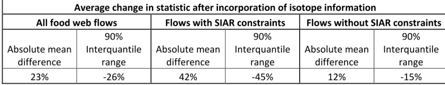
Sixty-four of the 175 flows in the Isotope LIM were constrained using SIAR-derived dietary constraints. The mean value for each flow and the corresponding 90% interquantile range (95% credible interval value – 5% credible interval value) are presented in Table 3. Seventy-nine (45%) and 43 (24%) of the means for the 175 flows were different between the Isotope and the Traditional LIMs by at least 10% and 25%, respectively (Table 3). Of the 64 flows which were constrained with SIAR-derived dietary constraints, 50 had their means change by at least 10%, and 31 had their means change by at least 25%. On average, all flows had a 23% absolute mean difference for the Isotope LIM in comparison with the Traditional; similarly the 90% interquantile ranges of the flows were reduced by 26% for the Isotope LIM in comparison with the Traditional LIM (Table 4). Flows constrained in the Isotope LIM using SIAR-derived diet constraints had, on average, a 42% absolute mean difference in comparison with the corresponding Traditional LIM flows, and their 90% interquantile ranges were reduced 45%. Additionally, the remaining 111 flows (those that were not directly constrained with SIAR-derived diet constraints in the Isotope LIM) had, on average, a 12% absolute mean difference, and 90% interquantile ranges were reduced by 15% on average.
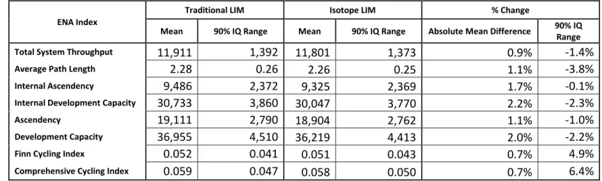
All network indices (total system throughput, average path length, internal ascendency, internal development capacity, ascendency, development capacity, Finn
cycling index and comprehensive cycling index) calculated from the Traditional and Isotope LIMs had small differences in their means (Table 5). Changes in the 90% interquantile ranges with the addition of the SIAR-derived isotope constraints in the Isotope LIM were small when compared with the Traditional LIM (Table 5).
4. DISCUSSION
4.1 Comparison of single flows and integrative indices between LIMs
Both individual flows and integrative indices as calculated from ENA parameters were changed as a result of the addition of the SIAR-derived dietary constraints in the Isotope LIM. However, the comparison of the ENA indices showed smaller differences in the means, uncertainty (90% interquantile ranges), and marginal probability
distributions between the Traditional and Isotope LIMs when compared to those differences between individual flows. This agrees with the findings of Kones et al. (2009), who found that whole network indices are better constrained and more robust than the food webs from which they are calculated. Differences between the two models were more apparent when looking at the individual flow level as compared to a more aggregate, whole system measure (i.e., ENA indices). This suggests that the integration of the stable isotope data has the largest effect when looking at specific flows within the food web. Linear inverse models are most often utilized to quantify systems with a large number of unknown flows and data deficiencies. The fact that the integrative indices calculated from the Traditional and Isotope LIMs show small differences suggests that the LIM-MCMC technique is a robust method for assessing whole-ecosystem properties, even in the absence of site-specific stable isotope data.
Generally, the largest differences seen between the Traditional and Isotope LIMs were in those flows which were directly constrained by SIAR-derived diet constraints (Table 4). However, flows not directly constrained with isotope data were still affected, as evidenced by the reduced uncertainty and changes in means. This demonstrates the interconnected nature of the food web, as well as how constraining some flows with isotope data can have widespread effects on reducing uncertainty in LIM-MCMC models.
4.2 Integration of stable isotope data in food web models
The goal of this study was to find a way to incorporate information from multiple
stable isotope elements (i.e., 13C, 15N, etc.) into food web models using the LIM-MCMC
technique, with minimum added complexity. The technique of using SIAR-derived food
source contribution constraints successfully integrated δ13C and δ15N information into the
LIM-MCMC models. Analysis of LIM-MCMC output showed the Isotope LIM to be significantly different, as well as significantly more precise, than the Traditional LIM.
Thus, the integration of δ13C and δ15N data into the food web model through isotope
mixing model diet constraints succeeded in reducing the uncertainty of the food web
model solution. Van Oevelen et al. (2006) found, similarly, that inclusion of δ13C data
significantly constrained a conventional LIM of a benthic intertidal flat food web. This study builds on this finding by simultaneously including stable isotope information from
two markers (δ13C and δ15N), as well as using stochastic techniques to fully describe the
food web model solution space and associated uncertainty.
The use of the SIAR mixing models allowed for incorporation of uncertainty in both the measured stable isotope values, as well as the fractionation factors.
Incorporating the 90% credible intervals from the mixing models into the LIM-MCMC in the form of inequalities agrees well with conventional practices for building linear
inverse models and is relatively simple to do, but comes at the cost of losing information regarding the tails of the marginal posterior distributions. Future models may choose to incorporate this information in a similar fashion to Hosack and Eldridge (2009), though this would add significant complexity. This methodology allows for data from multiple isotopic markers to be used in order to estimate contributions from all likely food sources
to each consumer. It is well established that a multiple marker approach (δ13C and δ15N)
is significantly more informative when estimating diet contributions when compared to a
single marker (δ13C or δ15N) (Parnell et al., 2012; Phillips, 2012). Due to this, use of
stable isotope mixing models in ecosystem-level food web studies can be advantageous for quantifying consumption flows. These same food web flows are often the most difficult to directly observe and measure as well, making isotopic mixing models a powerful tool for coupling with ecosystem-level food web models. This study used
only two isotopic markers (δ13C and δ15N), as this was the only data available at the time,
although the SIAR mixing models allow for incorporation of more than two (Parnell et al., 2010). However, use of isotopic mixing models utilizing more than three markers becomes problematic, as it is difficult to determine the model fit and visualize the mixing space (this would require > three dimensions) (Parnell et al., 2012).
Additionally, the use of the stable isotope mixing models helped validate the a priori food web model by verifying that the consumer diet networks were possible, and not missing a potential food source as indicated by the isotope data. While no statistical test exists for missing food sources (Parnell et al., 2012), visualization of the iso-space
for food web compartments is a tool that ecologists can use to identify probable predator-prey relationships. As mentioned, multiple isotopic markers help to better elucidate these relationships. Perhaps most importantly, though, is the fact that the stable isotope data specifically constrain consumption flows, which are often the most difficult to obtain reliable data on. This difficulty in obtaining reliable data leads to many ecosystem network models using diet data not specific to the study site of interest, such as from databases like FishBase (www.fishbase.org) (Coll et al., 2011). This can be a dangerous practice, as it has been shown that there can be considerable inter-site variability in the diet of members of the same species. We recommend the use of local diet information in the construction of food web models, as can be provided by mixing models utilizing site-specific stable isotope markers. It is important to note that stable isotope data obtained from the literature or other sites is not useful when building a food web model, as values are site-specific and only comparable within the site and appropriate temporal period from which the stable isotope samples were gathered.
4.3 Effects of SIAR-derived food source constraints on the modeled food web
Integration of mixing model constraints into LIM-MCMC models address an obvious weakness of stable isotope mixing models: current commonly used mixing models do not take into account the availability of food sources (Parnell et al., 2010; Phillips and Gregg, 2003; Semmens et al., 2009). Mixture partitioning is dictated purely by the stable isotope signatures of the consumer and food sources, regardless of whether or not there are enough of those food sources in the system to support the level of consumption suggested by the mixing model. The LIM-MCMC model deals with this
issue through mass balance of each compartment, and incorporating field-measured biomass estimates for each compartment into the model. This constrains the biomass of each compartment in the model, and therefore the amount available for consumption. While a simple concept, this is nonetheless an important attribute of ecosystem models, and an example of how the combination of isotope mixing models with inverse food web models is quite beneficial.
The use of the Markov-Chain Monte Carlo method (van Oevelen et al., 2010) to solve the models enabled the statistical comparison to be done between the Traditional and Isotope models. Previous techniques, which relied on minimization of an objective function to choose one answer for a model, did not allow for statistically rigorous comparisons between models (Vezina and Platt, 1988). Comparison of the mPDFs of each flow allowed for utilization of all solution data from the models, as well as taking into account the uncertainty associated with each flow. The same concept applied to the comparisons of the ENA indices. The LIM-MCMC technique also allows for the repeatability of model solutions, which is imperative for future comparative ecosystem studies.
Acknowledgments:
The present study was carried out at the University of La Rochelle, France and Oregon State University, United States, and partially funded by the European research programs PNEC, EC2CO, COMPECO, ORIQUART, and the Région Poitou Charentes. We are grateful to all of our colleagues who made data available and helped with the modeling process, including Boutheina Grami, Blanche Saint-Béat, and Geoffrey R.
Hosack. This document has been subjected to review by the National Health and Environmental Effects Research Laboratory’s Western Ecology Division and approved for publication. Approval does not signify that the contents reflects the views of the Agency, nor does mention of trade names or commercial products constitute endorsement or recommendation for use.
Baeta, A., Niquil, N., Marques, J.C., Patrício, J., 2011. Modelling the effects of eutrophication, mitigation measures and an extreme flood event on estuarine benthic food webs. Ecological Modelling 222, 1209–1221.
Baird, D., Asmus, H., Asmus, R., 2004. Energy flow of a boreal intertidal ecosystem, the Sylt-Rømø Bight. Mar. Ecol. Prog. Ser 279, 45–61.
Baird, D., Fath, B., Ulanowicz, R., Asmus, H., 2009. On the consequences of aggregation and balancing of networks on system properties derived from ecological network analysis. Ecological Modelling 279, 45-61.
Banašek-Richter, C., Cattin, M.-F., Bersier, L.-F., 2004. Sampling effects and the robustness of quantitative and qualitative food-web descriptors. Journal of Theoretical Biology 226, 23–32.
Breed, G., Jackson, G., Richardson, T., 2004. Sedimentation, carbon export and food web structure in the Mississippi River plume described by inverse analysis. Mar. Ecol. Prog. Ser 278, 35–51.
Christensen, V., Pauly, D., 1992. Ecopath II—a software for balancing steady-state ecosystem models and calculating network characteristics. Ecological Modelling 61, 169–185.
Christian, R., Brinson, M., Dame, J., Johnson, G., 2009. Ecological network analyses and their use for establishing reference domain in functional assessment of an estuary. Ecological Modelling 220, 3113-3122.
Coll, M., Schmidt, A., Romanuk, T., Lotze, H.K., 2011. Food-Web Structure of Seagrass Communities across Different Spatial Scales and Human Impacts. PLoS One 6, e22591.
Daniels, R., Richardson, T., Ducklow, H., 2006. Food web structure and biogeochemical processes during oceanic phytoplankton blooms: an inverse model analysis. Deep Sea Research Part II: Topical Studies in Oceanography 53, 532–554.
Degré, D., Leguerrier, D., Armynot du Chatelet, E., Rzeznik, J., Auguet, J., Dupuy, C., Marquis, E., Fichet, D., Struski, C., Joyeux, E., 2006. Comparative analysis of the food webs of two intertidal mudflats during two seasons using inverse modelling: Aiguillon Cove and Brouage Mudflat, France. Estuarine, Coastal and Shelf Science 69, 107–124.
Donali, E., Olli, K., Heiskanen, A., Andersen, T., 1999. Carbon flow patterns in the planktonic food web of the Gulf of Riga, the Baltic Sea: a reconstruction by the inverse method. Journal of Marine Systems 23, 251–268.
Eldridge, P., Cifuentes, L., Kaldy, J., 2005. Development of a stable-isotope constraint system for estuarine food-web models. Mar. Ecol. Prog. Ser 303, 73–90.
Eldridge, P., Jackson, G., 1993. Benthic trophic dynamics in California coastal basin and continental slope communities inferred using inverse analysis. Mar. Ecol. Prog. Ser 99, 115–115.
Fath, B.D., Scharler, U.M., Ulanowicz, R.E., Hannon, B., 2007. Ecological network analysis: network construction. Ecological Modelling 208, 49–55.
Grami, B., Niquil, N., Sakka Hlaili, A., Gosselin, M., Hamel, D., Hadj Mabrouk, H., 2008. The plankton food web of the Bizerte Lagoon (South-western Mediterranean): II. Carbon steady-state modelling using inverse analysis. Estuarine, Coastal and Shelf Science 79, 101–113.
Functional Effects of Parasites on Food Web Properties during the Spring Diatom Bloom in Lake Pavin: A Linear Inverse Modeling Analysis. PLoS One 6, e23273. Hosack, GR and PM Eldridge. 2009. Do microbial processes regulate the stability of a coral atoll's enclosed pelagic ecosystem? Ecological Modelling 220, 2665-2682. Jackson, G., Eldridge, P., 1992. Food web analysis of a planktonic system off Southern
California. Progress in Oceanography 30, 223–251.
Johnson, G., Niquil, N., Asmus, H., Bacher, C., 2009. The effects of aggregation on the performance of the inverse method and indicators of network analysis. Ecological Modelling 220, 3448-3464.
Kones, J., Soetaert, K., van Oevelen, D., Owino, J., 2009. Are network indices robust indicators of food web functioning? a monte carlo approach. Ecological Modelling 220, 370–382.
Kones, J., Soetaert, K., van Oevelen, D., Owino, J., Mavuti, K., 2006. Gaining insight into food webs reconstructed by the inverse method. Journal of Marine Systems 60, 153–166.
Lebreton, B., Richard, P., Galois, R., Radenac, G., Brahmia, A., Colli, G., Grouazel, M., André, C., Guillou, G., Blanchard, G.F., 2012. Food sources used by sediment
meiofauna in an intertidal Zostera noltii seagrass bed: a seasonal stable isotope study. Marine Biology 159, 1537-1550.
Lebreton, B., Richard, P., Radenac, G., Bordes, M., Breret, M., Arnaud, C., Mornet, F., Blanchard, G., 2009. Are epiphytes a significant component of intertidal Zostera noltii beds? Aquatic Botany 91, 82–90.
comparison of two intertidal mudflat food webs (Brouage Mudflat and Aiguillon Cove, SW France). Estuarine, Coastal and Shelf Science 74, 403–418.
Leguerrier, D., Niquil, N., Boileau, N., Rzeznik, J., Sauriau, P., Le Moine, O., Bacher, C., 2003. Numerical analysis of the food web of an intertidal mudflat ecosystem on the Atlantic coast of France. Mar. Ecol. Prog. Ser 246, 17–37.
Leguerrier, D., Niquil, N., Petiau, A., Bodoy, A., 2004. Modeling the impact of oyster culture on a mudflat food web in Marennes-Oléron Bay (France). Mar. Ecol. Prog. Ser. 273, 147–161.
Leslie, H.M., McLeod, K.L., 2007. Confronting the challenges of implementing marine ecosystem-based management. Frontiers in Ecology and the Environment 5, 540– 548.
Moore, J., Semmens, B., 2008. Incorporating uncertainty and prior information into stable isotope mixing models. Ecology Letters 11, 470–480.
Navarro, J., Coll, M., Louzao, M., Palomera, I., Delgado, A., Forero, M., 2011. Comparison of ecosystem modelling and isotopic approach as ecological tools to investigate food webs in the NW Mediterranean Sea. Journal of Experimental Marine Biology and Ecology 401, 97-104.
Niquil, N., Bartoli, G., Urabe, J., Jackson, G., Legendre, L., Dupuy, C., Kumagai, M., 2006. Carbon steady-state model of the planktonic food web of Lake Biwa, Japan. Freshwater Biology 51, 1570–1585.
Niquil, N., Chaumillon, E., Johnson, G.A., Bertin, X., Grami, B., David, V., Bacher, C., Asmus, H., Baird, D., Asmus, R., 2012. The effect of physical drivers on ecosystem indices derived from ecological network analysis: Comparison across estuarine
ecosystems. Estuarine, Coastal and Shelf Science 108, 132–143.
Niquil, N., Jackson, G., Legendre, L., Delesalle, B., 1998. Inverse model analysis of the planktonic food web of Takapoto Atoll (French Polynesia). MEPS 165, 17–29. Oevelen, D., Meersche, K., Meysman, F.J.R., Soetaert, K., Middelburg, J.J., Vézina,
A.F., 2010. Quantifying Food Web Flows Using Linear Inverse Models. Ecosystems 13, 32–45.
Parnell, A., Inger, R., Bearhop, S., Jackson, A., 2010. Source partitioning using stable isotopes: coping with too much variation. PLoS One 5, e9672.
Parnell, A.C., Phillips, D.L., Bearhop, S., 2012. Bayesian Stable Isotope Mixing Models. arXiv:1209.6457v1.
Pauly, D., 2000. Ecopath, Ecosim, and Ecospace as tools for evaluating ecosystem impact of fisheries. ICES Journal of Marine Science 57, 697–706.
Phillips, D., Gregg, J., 2001. Uncertainty in source partitioning using stable isotopes. Oecologia 127, 171-179.
Phillips, D., Gregg, J., 2003. Source partitioning using stable isotopes: coping with too many sources. Oecologia 136, 261-269.
Phillips, D., Newsome, S., Gregg, J., 2005. Combining sources in stable isotope mixing models: alternative methods. Oecologia 144, 520-527.
Phillips, D.L., 2012. Converting isotope values to diet composition: the use of mixing models. Journal of Mammalogy 93, 342–352.
Post, D., 2002. Using stable isotopes to estimate trophic position: models, methods, and assumptions. Ecology 83, 703–718.
models: a response to Jacksonet al.(2009). Ecology Letters 12, E6–E8. Ulanowicz, R., 2004. Quantitative methods for ecological network analysis.
Computational Biology and Chemistry 28, 321–339.
Van den Meersche, K., Soetaert, K., van Oevelen, D., 2009. xsample (): An R Function for Sampling Linear Inverse Problems. Journal of Statistical Software, Code Snippets 30, 1–15.
van Oevelen, D., Soetaert, K., Middelburg, J., Herman, P., Moodley, L., Hamels, I., Moens, T., Heip, C., 2006. Carbon flows through a benthic food web: Integrating biomass, isotope and tracer data. Journal of Marine Research 64, 453–482. van Oevelen, D., Van den Meersche, K., Meysman, F., Soetaert, K., Middelburg, J.,
Vézina, A., 2010. Quantifying Food Web Flows Using Linear Inverse Models. Ecosystems 13, 32–45.
Vander Zanden, M.J., Rasmussen, J.B., 2001. Variation in δ15N and δ13C trophic fractionation: implications for aquatic food web studies. Limnology and Oceanography 46, 2061-2066.
Vezina, A., Platt, T., 1988. Food web dynamics in the ocean. 1. Best-estimates of flow networks using inverse methods. Marine Ecology Progress Series. Oldendorf 42, 269–287.
Walters, C., Christensen, V., Pauly, D., 1997. Structuring dynamic models of exploited ecosystems from trophic mass-balance assessments. Reviews in fish biology and fisheries 7, 139–172.
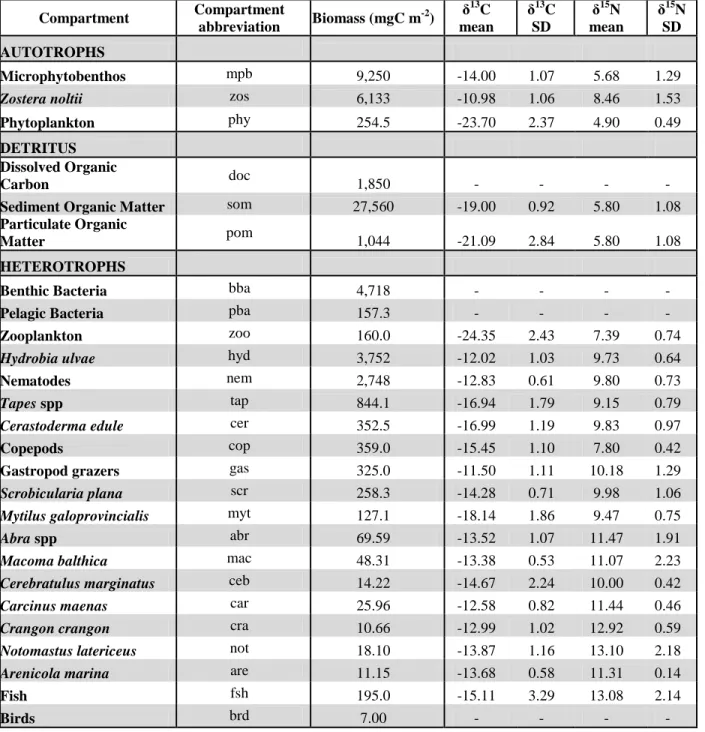
Table 1. Food web compartments, along with their biomasses and stable isotope values used in the Traditional and Isotope LIMs.
Compartment Compartment abbreviation Biomass (mgC m -2) δ13C mean δ13 C SD δ15 N mean δ15 N SD AUTOTROPHS Microphytobenthos mpb 9,250 -14.00 1.07 5.68 1.29
Zostera noltii zos 6,133 -10.98 1.06 8.46 1.53
Phytoplankton phy 254.5 -23.70 2.37 4.90 0.49
DETRITUS
Dissolved Organic
Carbon doc 1,850 - - - -
Sediment Organic Matter som 27,560 -19.00 0.92 5.80 1.08
Particulate Organic
Matter pom 1,044 -21.09 2.84 5.80 1.08
HETEROTROPHS
Benthic Bacteria bba 4,718 - - - -
Pelagic Bacteria pba 157.3 - - - -
Zooplankton zoo 160.0 -24.35 2.43 7.39 0.74
Hydrobia ulvae hyd 3,752 -12.02 1.03 9.73 0.64
Nematodes nem 2,748 -12.83 0.61 9.80 0.73
Tapes spp tap 844.1 -16.94 1.79 9.15 0.79
Cerastoderma edule cer 352.5 -16.99 1.19 9.83 0.97
Copepods cop 359.0 -15.45 1.10 7.80 0.42
Gastropod grazers gas 325.0 -11.50 1.11 10.18 1.29
Scrobicularia plana scr 258.3 -14.28 0.71 9.98 1.06
Mytilus galoprovincialis myt 127.1 -18.14 1.86 9.47 0.75
Abra spp abr 69.59 -13.52 1.07 11.47 1.91
Macoma balthica mac 48.31 -13.38 0.53 11.07 2.23
Cerebratulus marginatus ceb 14.22 -14.67 2.24 10.00 0.42
Carcinus maenas car 25.96 -12.58 0.82 11.44 0.46
Crangon crangon cra 10.66 -12.99 1.02 12.92 0.59
Notomastus latericeus not 18.10 -13.87 1.16 13.10 2.18
Arenicola marina are 11.15 -13.68 0.58 11.31 0.14
Fish fsh 195.0 -15.11 3.29 13.08 2.14
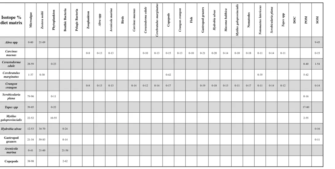
Table 2. SIAR-derived dietary contribution matrix. Lower and upper bounds of the 90% credible intervals are given, with consumers by row and prey items by column. Values are in units of percent contribution to total diet.
Isotope % diet matrix M icr oalgae Z os ter a n olt ii P h y top lan k to n B en th ic B ac te ria P elagi c B ac te ria Z oop la n k ton A br a s p p A re n icola mar in a B irds C ar cin u s maenas C er as toder ma edu le C er ebr atu lu s mar gin at u s Copepo d s C ran gon c ran go n F is h Gas tr op o d gr az er s Hydr obia u lvae M ac oma balt h ica M yti lu s galopr ov in c ial is Ne m at o d es Notomas tu s lat er ice u s S cr obicul ar ia pl an a T ape s sp p DOC POM SOM Abra spp 0-60 21-69 9-45 Carcinus maenas 0-8 0-13 0-13 0-10 0-13 0-15 0-13 0-10 0-21 0-20 0-14 0-10 0-18 0-11 0-14 0-11 0-15 Cerastoderma edule 28-59 0-23 0-40 1-54 Cerebratulus marginatus 1-37 0-30 0-42 0-35 5-42 Crangon crangon 0-8 0-13 0-13 0-14 0-12 0-14 0-17 0-19 0-18 0-13 0-11 0-17 0-11 0-14 0-12 0-14 Scrobicularia plana 79-96 0-11 0-16 Tapes spp 39-65 0-22 17-60 Mytilus galoprovincialis 22-52 10-55 2-55 Hydrobia ulvae 12-53 34-70 0-24 0-16 Gastropod grazers 21-34 59-83 0-14 0-11 Arenicola marina 0-41 21-60 21-56 Copepods 38-98 2-62
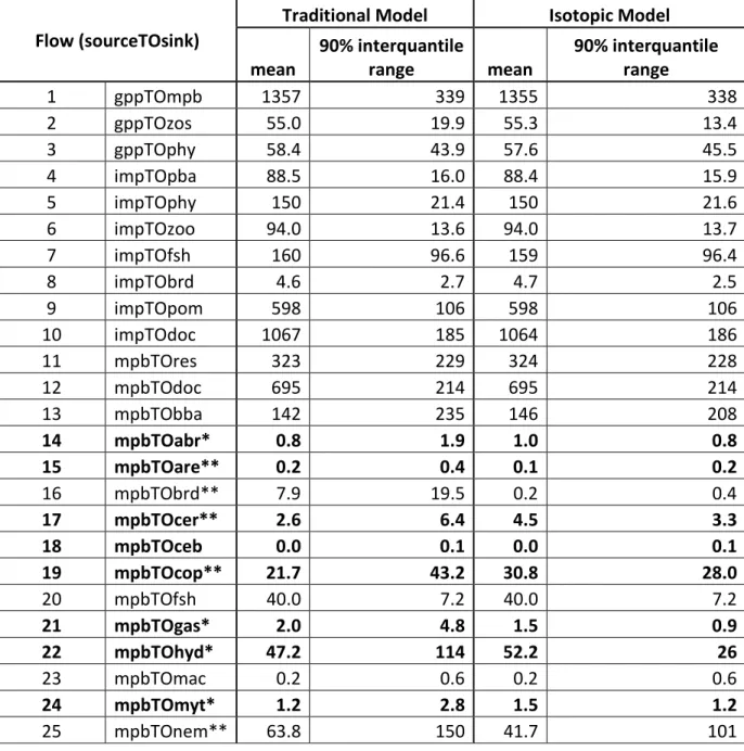
Table 3. Flow means and 90% interquantile ranges of the Traditional and Isotope LIMs. Statistics are calculated with n=50,000 for each model (the number of Monte-Carlo
simulations). 90% interquantile ranges are calculated as the 95% quantile value minus the 5%
interquantile value. Units are mg C m-2 d-1. Each flow is composed of the abbreviation of the
source compartment (see table 1) TO the abbreviation of the sink compartment. gpp = gross primary production, imp = import, exp = export and res = respiration.
Flow (sourceTOsink)
Traditional Model Isotopic Model mean 90% interquantile range mean 90% interquantile range 1 gppTOmpb 1357 339 1355 338 2 gppTOzos 55.0 19.9 55.3 13.4 3 gppTOphy 58.4 43.9 57.6 45.5 4 impTOpba 88.5 16.0 88.4 15.9 5 impTOphy 150 21.4 150 21.6 6 impTOzoo 94.0 13.6 94.0 13.7 7 impTOfsh 160 96.6 159 96.4 8 impTObrd 4.6 2.7 4.7 2.5 9 impTOpom 598 106 598 106 10 impTOdoc 1067 185 1064 186 11 mpbTOres 323 229 324 228 12 mpbTOdoc 695 214 695 214 13 mpbTObba 142 235 146 208 14 mpbTOabr* 0.8 1.9 1.0 0.8 15 mpbTOare** 0.2 0.4 0.1 0.2 16 mpbTObrd** 7.9 19.5 0.2 0.4 17 mpbTOcer** 2.6 6.4 4.5 3.3 18 mpbTOceb 0.0 0.1 0.0 0.1 19 mpbTOcop** 21.7 43.2 30.8 28.0 20 mpbTOfsh 40.0 7.2 40.0 7.2 21 mpbTOgas* 2.0 4.8 1.5 0.9 22 mpbTOhyd* 47.2 114 52.2 26 23 mpbTOmac 0.2 0.6 0.2 0.6 24 mpbTOmyt* 1.2 2.8 1.5 1.2 25 mpbTOnem** 63.8 150 41.7 101
26 mpbTOnot 0.4 0.8 0.4 0.8 27 mpbTOscr** 2.0 4.7 5.3 1.9 28 mpbTOtap** 6.9 15.7 10.6 6.2 29 zosTOres** 10.9 15.2 7.5 13.4 30 zosTOdoc** 2.0 2.4 0.9 0.3 31 zosTOexp** 5.7 15.2 0.1 0.2 32 zosTOsom** 5.8 15.6 0.1 0.2 33 zosTOabr** 0.8 1.8 0.6 0.3 34 zosTOare 0.2 0.4 0.2 0.1 35 zosTObrd** 22.8 23.7 0.4 0.5 36 zosTOceb** 0.0 0.1 0.0 0.0 37 zosTOgas** 1.6 4.1 3.5 0.5 38 zosTOhyd** 5.4 14.7 42.2 0.5 39 phyTOres 11.3 18.2 11.2 18.2 40 phyTOdoc 6.1 4.2 6.0 4.4 41 phyTOexp 139 21.3 140 21.5 42 phyTOpom* 24.2 44.5 29.5 48.6 43 phyTOcer** 2.6 6.3 1.2 2.2 44 phyTOmac 0.2 0.6 0.2 0.6 45 phytOmyt** 1.2 2.8 0.8 1.4 46 phyTOscr** 2.0 4.6 0.3 0.6 47 phyTOtap** 6.5 15.1 2.2 4.2 48 phyTOzoo* 14.6 35.0 16.2 38.5 49 docTOexp 1036 185 1038 185 50 docTOpba 72.5 162 72.8 162 51 docTObba 937 426 937 423 52 pomTOexp 348 456 367 456 53 pomTOsom 436 403 433 407 54 pomTOcer* 2.6 6.5 2.0 3.7 55 pomTOmac 0.2 0.6 0.2 0.6 56 pomTOmyt* 1.3 2.8 1.5 1.9 57 pomTOpba 87.9 176 86.2 174 58 pomTOscr** 2.1 4.6 0.5 0.9 59 pomTOtap 7.1 15.9 7.7 7.0 60 pomTOzoo 21.6 54.1 21.1 53.5 61 somTOexp 167 392 172 398 62 somTOpom 166 399 169 401 63 somTOabr* 0.8 1.9 0.7 0.7 64 somTObba 237 416 218 397
65 somTOcar 0.1 0.2 0.1 0.1 66 somTOceb* 0.0 0.1 0.0 0.1 67 somTOcer 2.6 6.4 2.7 4.5 68 somTOcra 0.1 0.2 0.1 0.1 69 somTOgas** 2.0 4.8 0.3 0.6 70 somTOhyd** 49.0 118 10.9 18 71 somTOmac 0.2 0.6 0.2 0.6 72 somTOnot 0.4 0.8 0.4 0.8 73 bbaTOres 626 234 623 220 74 bbaTOdoc 103 50.9 103 50.8 75 bbaTOare* 0.2 0.4 0.2 0.2 76 bbaTOcop** 25.3 44.0 16.2 26.6 77 bbaTOgas** 2.0 4.8 0.4 0.7 78 bbaTOhyd** 72.0 135 18.5 24 79 bbaTOnem* 487 170 540 107 80 pbaTOres 38.7 92.4 38.7 92.5 81 pbaTOdoc 44.0 99.9 43.4 99.2 82 pbaTOexp 90.3 16.0 90.3 16.0 83 pbaTOzoo 75.9 62.3 75.1 62.7 84 zooTOres 51.7 16.6 51.8 16.5 85 zooTOdoc 35.4 32.7 35.6 32.8 86 zooTOexp 88.0 13.7 88.0 13.7 87 zooTOpom 10.4 21.4 10.4 21.4 88 zooTOcar** 0.1 0.2 0.0 0.1 89 zooTOcra** 0.1 0.2 0.0 0.1 90 zooTOfsh 20.5 26.7 20.5 26.7 91 abrTOres 1.3 0.2 1.3 0.2 92 abrTOsom* 0.9 0.8 0.7 0.7 93 abrTOcar 0.1 0.2 0.1 0.1 94 abrTOcra 0.1 0.2 0.1 0.1 95 abrTOfsh 0.1 0.2 0.1 0.2 96 areTOres 0.2 0.0 0.2 0.0 97 areTOsom 0.2 0.1 0.2 0.1 98 areTObrd* 0.0 0.0 0.0 0.0 99 areTOcar* 0.0 0.0 0.0 0.0 100 areTOcra* 0.0 0.0 0.0 0.0 101 areTOfsh 0.0 0.0 0.0 0.0 102 brdTOres** 24.3 29.1 0.7 1.3 103 brdTOsom** 14.6 19.2 0.4 0.6
104 brdTOexp 4.5 2.7 4.3 2.5 105 carTOres 0.4 0.1 0.4 0.1 106 carTOsom 0.4 0.2 0.4 0.2 107 carTOcra** 0.0 0.1 0.1 0.1 108 carTofsh* 0.1 0.1 0.1 0.1 109 cerTOres 5.3 0.6 5.3 0.6 110 cerTOsom 3.8 3.2 3.8 3.2 111 cerTOcar** 0.1 0.2 0.0 0.1 112 cerTOcra* 0.1 0.2 0.1 0.1 113 cerTOfsh 1.1 0.4 1.1 0.3 114 cebTOres 0.1 0.0 0.1 0.0 115 cebTOsom 0.1 0.1 0.1 0.0 116 cebTOcar 0.0 0.0 0.0 0.0 117 cebTOcra 0.0 0.0 0.0 0.0 118 cebTOfsh 0.0 0.0 0.0 0.0 119 copTOres 26.7 3.4 26.7 3.4 120 copTOdoc 12.4 17.0 12.5 17.0 121 copTOsom 7.7 16.3 7.7 16.3 122 copTOcar 0.1 0.2 0.1 0.1 123 copTOceb* 0.0 0.1 0.0 0.1 124 copTOcra* 0.1 0.2 0.1 0.1 125 craTOres 0.4 0.1 0.4 0.1 126 craTOsom 0.4 0.2 0.4 0.2 127 craTOcar* 0.0 0.1 0.0 0.1 128 craTOfsh* 0.0 0.1 0.0 0.1 129 fshTOres 160 79.6 164 74.6 130 fshTOpom 108 91.2 112 92.9 131 fshTOexp 172 95.4 174 95.3 132 fshTOcar** 0.1 0.2 0.0 0.1 133 gasTOres* 3.5 0.9 3.0 0.3 134 gasTOsom** 2.5 2.1 1.3 0.4 135 gasTOcar** 0.1 0.2 0.1 0.2 136 gasTOcra** 0.1 0.2 0.1 0.2 137 gasTOfsh* 1.4 0.5 1.2 0.4 138 hydTOres* 83.0 18.1 71.9 0.6 139 hydTOsom** 59.9 49.8 26.2 0.7 140 hydTObrd** 8.1 19.8 0.1 0.3 141 hydTOcar** 0.1 0.2 0.1 0.2 142 hydTOcra* 0.1 0.2 0.1 0.1
143 hydTOfsh* 22.3 22.6 25.4 0.7 144 macTOres 0.5 0.0 0.5 0.0 145 macTOsom 0.3 0.3 0.3 0.3 146 macTOcar* 0.0 0.1 0.0 0.1 147 macTOcra* 0.0 0.1 0.0 0.1 148 macTOfsh* 0.0 0.1 0.0 0.1 149 mytTOres 1.9 0.2 1.9 0.2 150 mytTOsom 1.4 1.2 1.4 1.2 151 mytTOcar** 0.1 0.2 0.0 0.1 152 mytTOcra** 0.1 0.2 0.0 0.1 153 mytTOfsh* 0.3 0.3 0.3 0.2 154 nemTOres 198 71.4 207 49.7 155 nemTOdoc 80.8 158 87.4 166 156 nemTOsom 80.8 158 88.5 167 157 nemTOcar** 0.1 0.2 0.1 0.2 158 nemTOceb 0.0 0.1 0.0 0.1 159 nemTOcra* 0.1 0.2 0.1 0.1 160 nemTOfsh 192 87.9 199 85.8 161 notTOres 0.4 0.1 0.4 0.1 162 notTOsom 0.3 0.3 0.3 0.3 163 notTOcar* 0.0 0.1 0.0 0.1 164 notTOcra* 0.0 0.1 0.0 0.1 165 notTOfsh* 0.1 0.1 0.0 0.1 166 scrTOres 3.2 0.2 3.2 0.2 167 scrTOsom 2.2 1.9 2.2 1.9 168 scrTOcar 0.1 0.2 0.1 0.1 169 scrTOcra 0.1 0.2 0.1 0.1 170 scrTOfsh 0.6 0.3 0.6 0.2 171 tapTOres 10.8 0.7 10.8 0.7 172 tapTOsom 7.6 6.4 7.6 6.4 173 tapTOcar** 0.1 0.2 0.0 0.1 174 tapTOcra* 0.1 0.2 0.1 0.1 175 tapTOfsh 2.1 0.6 2.1 0.5
Bold: flow with corresponding SIAR diet constraint
* means of Isotope and Traditional LIM >10% different ** means of Isotope and Traditional LIM >25% different
Table 4. Comparison of means and 90% interquantile ranges for the Traditional and Isotope LIMs. The absolute mean difference for each flow was calculated as the absolute value of the difference between Traditional and Isotope LIM mean flow values. Negative values indicate a reduction in the interquantile range of the Isotope LIM when compared with the Traditional LIM.
Average change in statistic after incorporation of isotope information
All food web flows Flows with SIAR constraints Flows without SIAR constraints
Absolute mean difference 90% Interquantile range Absolute mean difference 90% Interquantile range Absolute mean difference 90% Interquantile range 23% -26% 42% -45% 12% -15%
Table 5. Comparison of the means and 90% interquantile (IQ) ranges of the Ecological Network Analysis indices for each of the models. Negative values for the percent change of 90% IQ Range represent a reduction in the range of the Isotope LIM when compared with the Traditional LIM.
ENA Index
Traditional LIM Isotope LIM % Change
Mean 90% IQ Range Mean 90% IQ Range Absolute Mean Difference 90% IQ
Range
Total System Throughput 11,911 1,392 11,801 1,373 0.9% -1.4%
Average Path Length 2.28 0.26 2.26 0.25 1.1% -3.8%
Internal Ascendency 9,486 2,372 9,325 2,369 1.7% -0.1%
Internal Development Capacity 30,733 3,860 30,047 3,770 2.2% -2.3%
Ascendency 19,111 2,790 18,904 2,762 1.1% -1.0%
Development Capacity 36,955 4,510 36,219 4,413 2.0% -2.2%
Finn Cycling Index 0.052 0.041 0.051 0.043 0.7% 4.9%
Figure 1. Overview of Marennes-Oléron Estuary study site, including the intertidal seagrass bed that was modeled. Sampling locations indicated as HFS (High Flat Site) and LFS (Low Flat Site).
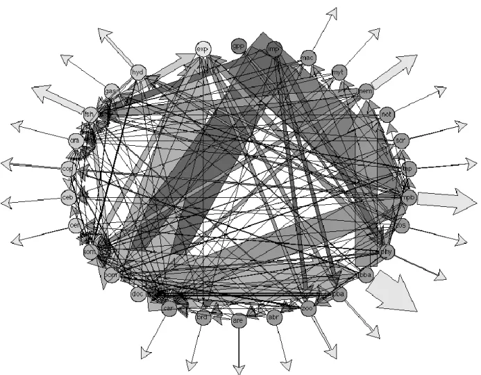
Figure 2. Food web diagram of the Marennes-Oléron intertidal seagrass system, formed using the mean flows from the Isotope
LIM. Width of arrows corresponds to relative magnitude of flow in units of mgC m-2 d-1. Arrows pointing away from center of