1015-1621/06/020154-18 DOI 10.1007/s00027-006-0813-x © Eawag, Dübendorf, 2006
Aquatic Sciences
Research Article
Distribution of diatoms, chironomids and cladocera
in surface sediments of thirty mountain lakes
in south-eastern Switzerland
Christian Bigler1,5,*
, Oliver Heiri2
, Renata Krskova3
, André F. Lotter2
and Michael Sturm4
1
University of Bern, NCCR Climate and Institute of Plant Sciences, Altenbergrain 21, CH-3013 Bern, Switzerland
2
Utrecht University, Palaeoecology, Laboratory of Palaeobotany and Palynology, Budapestlaan 4, 3584 CD Utrecht, the Netherlands
3
Charles University, Dept. of Hydrobiology, Vinicna 7, Praha 2, CZ-128 44, Czech Republic
4
Swiss Federal Institute for Environmental Science and Technology (Eawag), NCCR Climate and Dept. of Surface Waters (SURF), CH-8600 Dübendorf, Switzerland
5
Present address: Umeå University, Dept. of Ecology and Environmental Science, KBC plan 5, S-901 87 Umeå, Sweden
Received: 20 May 2005; revised manuscript accepted: 2 November 2005
Abstract. Surface sediments from 30 mountain lakes in
south-eastern Switzerland (Engadine, Grisons) were ana-lysed for subfossil diatom, chironomid, and cladoceran assemblages. Ordination techniques were used to identify relevant physical and chemical environmental parameters that best explain the distribution of these biota in the stud-ied lakes. Diatom assemblage composition showed a strong relationship with physical (e.g., lake depth, tem-perature, organic content of surface sediments) and chemi-cal variables (e.g., lake-water pH, alkalinity, silica concen-tration). The greatest variance in chironomid and cladoceran assemblages is explained by dissolved organic carbon (DOC) content of lake water, temperature, and the organic content of surface sediments, all parameters which
are highly correlated with lake elevation. Increasing lake depth is refl ected in diatom and cladoceran assemblages by higher percentages of planktonic species, whereas chi-ronomid assemblages in the deep Engadine lakes are char-acterised by a high proportion of lotic taxa. In contrast to similar studies in the Northern and Southern Alps, subfos-sil assemblages in the Engadine mountain lakes showed a strong relationship with DOC, which in these weakly buff-ered lakes is negatively correlated with altitude. According to our fi ndings, chironomid and cladocera remains have a considerable potential as quantitative palaeotemperature indicators in the Engadine area. This potential is somewhat weaker for diatoms which seem to be more strongly infl u-enced by water chemistry and lake bathymetry.
* Corresponding author phone: +46 90 786 97 29; fax: +46 90 786 67 05; e-mail: [email protected] Published Online First: May 17, 2006
Key words. Diatoms; chironomids; cladocera; mountain lakes; water chemistry; Engadine.
Introduction
Alpine and arctic lakes are increasingly affected by changing climatic and environmental conditions (Doug-las et al., 1994; Saros et al., 2003; Smol et al., 2005).
As a direct consequence of the global warming trend, an increase in lake-water temperatures and reduction of ice-cover duration is occurring, as both lake-water tem-peratures and the spring ice break-up dates are related to ambient air temperatures (Livingstone, 1997; Living-stone and Lotter, 1998). Furthermore, these lakes are in-fl uenced by indirect effects of increasing temperature, such as reduced snow cover in the catchment, increasing weathering rates, and increasing erosion
(Sommaruga-Wögrath et al., 1997). Moreover, airborne pollution (e.g., Wolfe et al., 2001) and other human-induced changes such as altered land-use patterns may be superimposed on climatic changes (Heiri and Lotter, 2003). In their combination, it is expected that these factors will exert a considerable infl uence on the physical and chemical structure of alpine and arctic lake ecosystems, and will act as substantial stressors to aquatic biota in these re-gions (Hinder et al., 1999; Rautio et al., 2000). However, due to the remote location of many arctic and alpine lakes and associated logistic constraints, it is often diffi cult to document biotic and abiotic changes on a regular moni-toring basis (e.g., Battarbee et al., 2002).
Palaeolimnological techniques offer the unique op-portunity to assess the lake response to historical envi-ronmental change and impacts of human activity (Ander-son and Battarbee, 1994; Smol, 2002). Both abiotic and biotic proxy-indicators of past environmental conditions are preserved in lake sediments and can be analysed to reconstruct past climatic variability (Lotter et al., 1997; Bigler et al., 2002), chemical conditions (Renberg et al., 1993; Lotter, 1998; Lotter et al., 1998) and biotic assem-blages in lakes (Uutula and Smol, 1996; Heiri et al., 2003). The interpretation of fossil assemblages, however, requires detailed knowledge on the modern occurrence of organisms and the relation of environmental gradients related to that distribution. A lack of ecological understanding of aquatic biota may cause considerable diffi -culties when interpreting fossil records in alpine and arctic areas. These alpine and arctic environments are those most important to understand, because they are particularly sensitive to global change (IPCC, 2001). There is a clear need for information on how climate changes have affected these regions in the past and on how alpine and arctic ecosystems are responding to changing environments.
The Engadine is an alpine valley situated in the east-ern Swiss Alps, that has been the focus of a number of palaeoenvironmental studies to reconstruct the history of human-induced nutrient enrichment (Züllig, 1982; Ariz-tegui and Dobson, 1996; ArizAriz-tegui et al., 1996; Lotter, 2001), glacial activity (e.g., Leemann and Niessen, 1994; Maisch et al., 2000), vegetation history (e.g., Gobet et al., 2003; Gobet, 2004) and to examine the relationships be-tween sedimentation processes and climate (Ohlendorf et al., 1997). However, these studies were carried out in the large lakes situated at the bottom of the Engadine Valley, whereas alpine lakes around the treeline ecotone, which have been shown to be well suited for organism-based environmental reconstruction (Lotter and Bigler, 2000; Hausmann et al., 2002; Lotter et al., 2002; Heiri et al., 2003) remain largely unexplored. A fi rst step to explore these lakes as palaeolimnological archives is to investi-gate their limnological characteristics and the distribu-tion of lacustrine biota. Whereas such extensive survey
data of small alpine lakes are available in the northern and southern Swiss Alps (Lotter et al., 1997; Lotter et al., 1998; Marchetto, 1998; Müller et al., 1998), they are largely missing from the eastern and central parts of the Swiss Alps.
In the following, we present a survey of lacustrine biota in the Engadine area. Subfossil assemblages of chi-ronomids, cladocerans and diatoms in the surface sedi-ment of 30 lakes ranging in elevation from 962 to 2815 m a.s.l. were analysed to assess the taxonomic composition of extant assemblages in subalpine and alpine lakes and to assess the distribution of these organisms with respect to major limnological and climatic parameters, which have been reported to have a strong infl uence on aquatic biota in the Swiss Alps (Lotter et al., 1997; Lotter et al., 1998). The study of subfossil material, however, puts some constraints on the achievable taxonomic resolution of the analyses. Nevertheless, fossil assemblages in sur-face sediment samples have the advantage of integrating biotic remains from the entire lake basin and over a number of years (Frey, 1988). They therefore provide a more comprehensive picture of the extant lacustrine fl ora and fauna than would otherwise be attainable except by intensive monitoring programs. Furthermore, surface sediment assemblages are directly comparable with the fossil record, an obvious advantage if the modern distri-bution of aquatic organisms is to be used to interpret palaeolimnological records. We concentrate on diatoms, chironomids and cladocerans as all of these organisms are diverse (Stoermer and Smol, 1999; Korhola and Rau-tio, 2001; Brooks, 2003), sensitive to limnological and climatic conditions (Lotter et al., 1997; Lotter et al., 1998) and represent different compartments of lake eco-systems (Frey, 1988). Furthermore, the remains of these organisms preserve well and remain identifi able in lake sediments and they are therefore valuable indicators of past environmental change (Battarbee et al., 2001; Ko-rhola et al., 2001; Walker, 2001).
Study area and sites
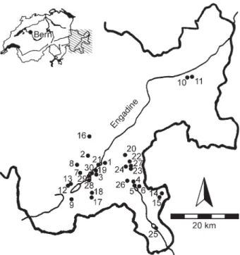
We sampled 30 lakes in south-eastern Switzerland (Grisons). Most of them are located in the Upper Enga-dine, and a few sites are in the Lower Engadine (TAR-10, and NAR-11) and the Poschiavo (VIO-14, SAO-15, and POS-25, Fig. 1). The climate in the Engadine is infl u-enced by air masses both from the south (i.e., the Medi-terranean Sea) and the north (i.e., the North Atlantic Ocean, Urfer et al., 1979). The sites cover broad gradi-ents in temperature and precipitation, as well as catch-ment vegetation types: some are located within the larch (Larix decidua) and stone pine (Pinus cembra) dominat-ed forests, whereas others are well above tree line and vegetation is sparse in the watershed (Table 1). The sam-pled lakes show considerable differences in lake mor-phometry (e.g., maximum lake depth) and catchment
size. In general the large, deep lakes (>30 m) are located in the valley bottom at lower altitudes (STM-21, POS-25, SIL-28, CHS-29, and CHN-30, see Table 1). The bedrock composition in the Upper Engadine consists predomi-nantly of granite and gneiss, with locally present calcare-ous intrusions lead to neutral (pH ~7) lake-water condi-tions in most lakes (Table 1).
Methods
Sampling and laboratory procedures
All lakes were sampled during August 2002, except SIL-28, CHS-29 and CHN-30, which were sampled in No-vember 2002. At each lake, we collected two one-litre water samples, the fi rst at 1-m water depth and the second
c. 1–3 m above the sediment surface, or, for deep lakes,
well below the thermocline (Table 1). The water samples were stored at 4 °C in glass bottles until analysis. A WTW Multi-line P4 (lakes #1–15) and EUTECH pH-Scan2 (lakes #16–30) pH meter was used for pH, and a WTW 330 LF conductivity meter for in situ measure-ments of conductivity and temperature. For both pH and conductivity, equipment was calibrated at each lake prior to measurements.
Further water chemistry analyses were carried out in the laboratories of the Swiss Federal Institute for Envi-ronmental Science and Technology (Eawag), Dübendorf. Alkalinity was measured by titration with strong acid to pH 4.3. Dissolved organic carbon (DOC) concentration was determined by thermal oxidation by a Shimatsu TOC-500 analyzer. Phosphate was determined photo-metrically with the molybdenum blue method, nitrate with the salicylic acid method, and silica (Si) with the molybdosilicate method (DEW, 1996). Total phospho-rous (TP) and total nitrogen (TN) were measured in unfi l-tered samples, after acidic digestion in an autoclave for
2 h at 120 ºC using K2S2O8. The detection limits for DOC,
TP and TN were 0.5 mg C L–1
, 5 µg P L–1
and 0.5 mg N L–1
, respectively.
We used July air temperature (July T) Climate Nor-mals (1961–1990) from the Swiss Meteorological Insti-tute (MeteoSwiss) corrected to sea level. For each lake site the average July T was calculated as the weighted mean of the three closest meteorological stations weight-ed by the inverse distance between lake and meteorologi-cal station. All values were corrected for altitude
apply-ing a lapse rate of 0.6 ºC 100 m–1
(Livingstone et al., 1999) before calculating the weighted average. In the Alps, air temperature and surface water temperature in lakes are closely correlated during the summer months (Livingstone et al., 1998; Livingstone et al., 1999), and mean air temperature can be estimated with a reasonably high accuracy even for remote alpine lakes during the summer months based on the available network of
mete-orological stations. Hence, summer air temperature is probably a more robust approximation of summer water temperature at our study sites than the spot measure-ments taken during fi eldwork.
Surface sediments were obtained in the deepest part of the lake basins using a modifi ed 80 mm diameter Ka-jak-corer (Renberg, 1991). Samples of 0–1, 1–2, and 2– 3 cm sediment depth were stored in NASCO whirl-paks and kept cool and dark until analysis. The organic content in the surface sediments was estimated using loss-on-ig-nition (LOI) and expressed as the percent weight loss af-ter combustion at 550 ºC for 4 h (Dean, 1974; Heiri et al., 2001).
Diatom preparation followed standard procedures
in-volving treatment with H2O2 (30 %) and HCl (10 %),
fol-lowed by heating for >7 h at 70 ºC (Battarbee, 1986). Af-ter rinsing the samples with distilled waAf-ter until pH was neutral, they were dried onto coverslips and permanently mounted using Naphrax mounting medium. Enumeration of diatoms (>500 frustules per sample) was done using a
Leica DMR microscope at 1000× magnifi cation with
phase contrast optics. Diatom taxonomy largely followed Krammer and Lange-Bertalot (1986–1991).
After defl occulation at room temperature in KOH (10 %) for 2 h, chironomid samples were sieved (100 µm mesh size) and chironomid remains were separated from
other remains under a stereo-microscope (40× magnifi
ca-tion). Chironomid head capsules were mounted in Euparal mounting medium after dehydration and identifi ed using a
microscope at 100×–400× magnifi cation. Identifi cation
Figure 1. Map of the study area showing the location of the sampled lakes. The lakes are numbered according to Table 1.
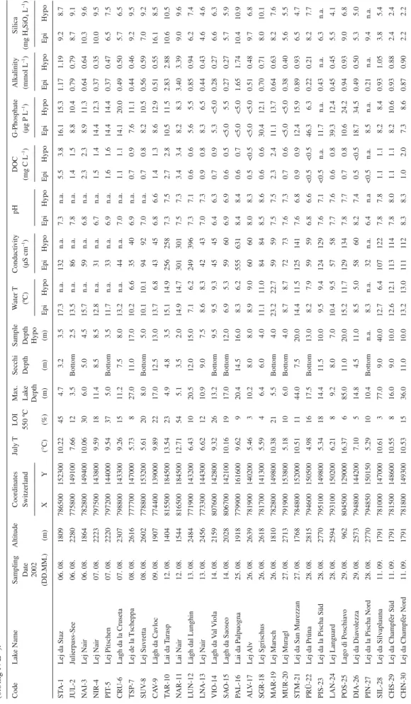
Ta
b
le 1.
Major en
vironmental v
ariables characterizing the sampled lak
es. G-Nitrate w
as belo
w the detection limit (<0.5
mg N L
–1) in all lak
es, e
x
cept in the epilimnion sample of CA
V -9 (0.6 mg N L –1). Code Lak e Name Sampling Altitude Coordinates July T LOI Max. Secchi Sample W ater T Conducti vity pH DOC G-Phosphate Alkalinity Silica Date Switzerland 550 ºC Lak e Depth Depth (ºC) (µS cm –1) (mg C L –1) (µg P L –1) (mmol L –1) (mg H 4 SiO 4 L –1) 2002 Depth Hypo (DD.MM.) (m) X Y (°C) (%) (m) (m) (m) Epi Hypo Epi Hypo Epi Hypo Epi Hypo Epi Hypo Epi Hypo Epi Hypo ST A-1 Lej da Staz 06. 08. 1809 786500 152300 10.22 45 4.7 3.2 3.5 17.3 n.a. 132 n.a. 7.3 n.a. 5.5 3.8 16.1 15.3 1.17 1.19 9.2 8.7 JUL-2 Julierpass-See 06. 08. 2280 775800 149100 7.66 12 3.5 Bottom 2.5 13.5 n.a. 86 n.a. 7.8 n.a. 1.4 1.5 8.8 10.4 0.79 0.79 8.7 9.1 NA I-3 Lej Nair 06. 08. 1864 782800 149400 10.06 30 6.0 5.0 4.5 15.7 n.a. 59 n.a. 6.8 n.a. 2.3 2.3 8.9 11.3 0.64 0.64 10.3 9.6 NIR-4 Lej Nair 07. 08. 2223 797500 143800 9.59 18 11.4 8.5 8.5 12.8 n.a. 31 n.a. 6.7 n.a. 1.5 1.4 14.4 12.3 0.37 0.35 10.0 9.5 PIT -5 Lej Pitschen 07. 08. 2220 797200 144000 9.54 37 5.0 Bottom 3.5 11.7 n.a. 33 n.a. 6.9 n.a. 1.6 1.6 14.4 14.4 0.37 0.47 6.5 7.5 CR U-6 Lagh da la Cruseta 07. 08. 2307 798800 143300 9.26 15 11.2 7.5 8.0 13.2 n.a. 44 n.a. 7.0 n.a. 1.1 1.1 14.1 20.0 0.49 0.50 5.7 6.5 TSP-7 Lej de la Tscheppa 08. 08. 2616 777700 147000 5.73 8 27.0 11.0 17.0 10.2 6.6 35 40 6.9 n.a. 0.7 0.9 7.6 11.1 0.44 0.46 9.2 9.5 SUV -8 Lej Suvretta 08. 08. 2602 778800 153200 5.61 20 8.0 Bottom 5.0 10.1 10.1 94 92 7.0 n.a. 0.7 0.8 8.2 10.5 0.56 0.59 7.0 9.2 CA V -9 Lägh da Ca vloc 09. 08. 1907 774400 139000 9.89 22 17.0 12.5 13.0 13.7 6.8 43 45 6.8 6.6 1.4 1.3 8.6 12.9 0.51 0.55 16.1 8.5 TA R-10 Lai da T arasp 12. 08. 1404 815500 184500 13.54 23 4.9 4.8 3.5 15.1 14.9 256 258 7.3 7.5 2.7 2.8 10.5 11.5 2.83 2.88 10.6 10.5 NA R-11 Lai Nair 12. 08. 1544 816500 184500 12.71 54 5.1 3.5 2.0 14.9 14.7 301 301 7.5 7.3 3.4 3.4 8.2 8.3 3.40 3.39 9.0 9.6 LUN-12 Lägh dal Lunghin 13. 08. 2484 771900 143200 6.43 10 20.5 12.0 15.0 7.1 6.2 249 396 7.3 7.1 0.6 0.6 5.6 5.5 0.85 0.94 6.2 7.4 LN A-13 Lej Nair 13. 08. 2456 773300 144300 6.62 12 10.9 9.0 7.5 8.6 8.3 42 43 7.0 7.3 0.9 0.8 8.3 6.5 0.44 0.43 4.6 4.6 VIO-14 Lagh da V al V iola 14. 08. 2159 807600 142800 9.32 26 13.2 Bottom 9.5 9.5 9.3 45 45 6.4 6.3 0.7 0.9 5.3 <5.0 0.28 0.27 6.6 6.3 SA O-15 Lagh da Saoseo 14. 08. 2028 806700 142100 10.16 19 17.0 Bottom 12.0 6.9 5.3 59 60 6.9 6.9 0.6 0.5 <5.0 5.5 0.27 0.27 5.7 5.9 PA L-16 Lai da P alpuogna 25. 08. 1918 779900 161600 9.62 9 20.4 14.5 16.0 8.3 6.2 555 631 8.4 8.4 0.6 0.7 <5.0 <5.0 1.65 1.74 10.4 10.9 AL V -17 Lej Alv 26. 08. 2639 781900 140200 5.46 3 10.2 8.0 8.0 8.9 9.0 60 60 8.0 8.3 0.5 <0.5 <5.0 <5.0 0.51 0.48 9.7 6.8 SGR-18 Lej Sgrischus 26. 08. 2618 781700 141300 5.59 4 6.4 6.0 4.0 11.1 11.0 84 84 8.5 8.6 0.6 0.6 30.4 12.1 0.70 0.71 8.0 10.1 MAR-19 Lej Marsch 26. 08. 1810 782800 149800 10.38 21 5.5 Bottom 4.0 23.2 22.7 59 59 7.5 7.5 2.3 2.4 11.1 13.7 0.64 0.63 8.2 7.6 MUR-20 Lej Muragl 27. 08. 2713 791900 153800 5.18 10 6.0 Bottom 4.0 8.7 8.7 72 73 7.6 7.3 0.7 0.6 <5.0 <5.0 0.38 0.40 5.6 5.5 STM-21 Lej da San Murezzan 27. 08. 1768 784800 152000 10.51 11 44.0 7.5 20.0 14.4 11.5 125 141 7.6 6.8 0.9 0.9 12.4 15.9 0.89 0.93 6.5 4.7 PRÜ-22 Lej da Prüna 28. 08. 2815 794600 150500 4.98 16 17.5 Bottom 13.0 8.2 7.9 59 59 6.8 6.6 <0.5 <0.5 46.3 6.3 0.22 0.21 8.2 7.7 PIS-23 Lej da la Pischa Süd 28. 08. 2770 795100 149800 5.34 18 14.4 11.5 10.0 9.5 9.4 124 129 7.6 7.1 <0.5 n.a. 11.7 n.a. 0.43 n.a. 6.3 n.a. LAN-24 Lej Languard 28. 08. 2594 793100 150200 6.21 8 9.2 8.0 7.0 10.4 9.5 57 58 7.7 7.6 0.6 0.8 39.3 12.4 0.45 0.45 5.5 4.1 POS-25 Lago di Poschia v o 29. 08. 962 804500 129000 16.37 6 85.0 11.0 20.0 15.2 11.7 129 134 7.8 7.7 0.7 0.8 10.6 24.2 0.94 0.93 9.0 6.8 DIA-26 Lej da Dia v o lezza 29. 08. 2573 794800 144200 7.10 5 14.8 4.5 11.0 8.5 5.0 58 60 8.2 7.4 0.5 <0.5 18.7 34.5 0.49 0.50 5.3 5.0 PIN-27
Lej da la Pischa Nord
28. 08. 2770 794850 150150 5.29 10 10.4 Bottom n.a. 8.3 n.a. 32 n.a. 6.4 n.a <0.5 n.a. 8.5 n.a. 0.21 n.a. 9.4 n.a. SIL-28 Lej da Silv aplauna 11. 09. 1791 781000 147000 10.61 3 77.0 9.0 40.0 12.7 6.4 107 122 7.8 7.8 1.1 1.1 8.2 8.4 0.93 1.05 3.8 5.4 CHS-29 Lej da Champfèr Süd 11. 09. 1791 781500 148600 10.55 8 16.0 9.0 10.0 12.6 12.1 113 114 7.8 8.0 1.1 1.1 8.2 10.6 0.93 0.88 2.4 2.4 CHN-30 Lej da Champfèr Nord 11. 09. 1791 781800 149300 10.53 15 36.0 11.0 10.0 13.2 13.0 111 112 8.3 8.3 1.0 2.0 7.3 8.6 0.87 0.90 2.2 2.2
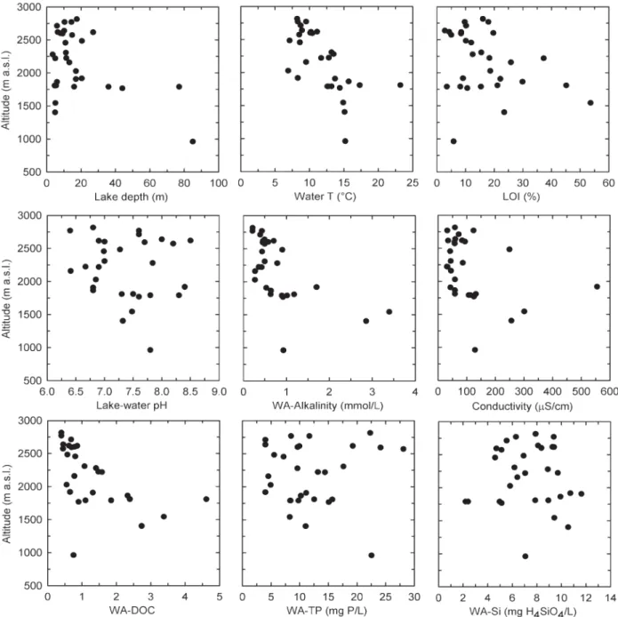
Figure 2. Major environmental variables in relation to the altitude of the study lakes.
was largely based on mentum characteristics described in Hofmann (1971), Wiederholm (1983) and Schmid (1993).
Thienemannimyia-type includes Tanypodinae head
cap-sules with a ventral and dorsal pore arrangement similar to
Conchapelopia, Rheopelopia, Telopelopia and Thiene-mannimyia in Rieradevall and Brooks (2001). Zavrelimyia
A features a pore arrangement on the head capsule as de-scribed by Heiri (2001). Tanytarsini head capsules were split into different categories following Heiri (2004) (for
Tanytarsus I-III, Micropsectra, Cladotanytarsus), Heiri
(2001) (for Paratanytarsus and Tanytarsus IV-VI) and Hofmann (1971) (for Tanytarsus lugens-type).
Cladoceran samples were prepared using standard methods (Frey, 1986; Prazakova and Fott, 1994; Korhola et al., 2001). Sediment was defl occulated using 10 % KOH and heated (approximately 70–80 ºC) for 0.5 h and subsequently sieved using 40 µm mesh size. Aliquots of
the residue were examined using a microscope at 100×
and 200× magnifi cation and identifi ed according to Frey
(1958; 1959), Korinek (1971) and Flössner (2000). The minimum number of exuviae of a given species in the samples was estimated based on the most abundant cladoceran skeletal fragment in the samples (Frey, 1986).
Numerical analyses
Diatom, chironomid and cladoceran taxa (Figs. 3–5) re-corded in less than three lakes were excluded for numeri-cal analyses. The percentage biologinumeri-cal data were square root transformed prior to numerical analyses in order to stabilise their variances. To assess whether to apply line-ar- or unimodal-based numerical techniques (ter Braak, 1986), we analysed each biological data set by Detrended Correspondence Analysis (DCA, Hill and Gauch, 1980), choosing the options detrending-by-segments, non-linear rescaling and downweighting of rare taxa (Fig. 6). As all analysed biological data sets have compositional gradient lengths of more than two standard deviation units, we used unimodal based species-response models (ter Braak and Prentice, 1988; Birks, 1995), i.e., Canonical Corre-spondence Analysis (CCA, ter Braak, 1986).
A series of partial CCAs was carried out with each environmental parameter as sole constraining variable to assess its explanatory power. For this purpose, we aver-aged the two water samples collected in each lake by applying a weighted averaging (WA) procedure for con-ductivity, DOC, TP, alkalinity, and silica as described by Lotter et al. (1998). For pH, we used measurements from 1 m water depth, as the application of WA procedure is not appropriate for parameters on a logarithmic scale. For parameters showing a skewed distribution in the 30 lake data set (i.e., LOI, water depth, conductivity, DOC, TP, alkalinity), log-transformation was applied before further numerical analysis. A TP dummy variable was created taking into account the differences of TP concentrations in epilimnion and hypolimnion, related to the minimum within the data set. The numerical treatments resulted in
PRÜ-22 PIN-27 PIS-23 MUR-20 ALV-17 SGR-18 TSP-07 SUV-08 LAN-24 DIA-26 LUN-12 LNA-13 CRU-06 JUL-02 NIR-04 PIT-05 VIO-14 SAO-15 PAL-16 CAV-09 NAI-03 MAR-19 STA-01 CHN-30 CHS-29 SIL-28 STM-21 NAR-11 TAR-10 POS-25 Lakes Frag ilaria capuci na var. aust riaca Cycl ostepha nos in visita tus 20 Aste rione lla formos a Frag ilaria crot onensi s 20 40 Cycl
otella cycl
opun cta 20 40 Tabel laria fl occu losa AGG . Navi cula d isjunct a Thala ssiosira ps eudon ana 20 Frag ilaria ulna var. acus 20 Frag ilaria const ruens var. bino dis 20 Step hano
discus parvus
Achnan thes minu tissi ma v ar. scot ica Navi cula vitio sa Cymbel la mi crocep hala 20 Achnan thes minu tissi ma Achnan thes leva nderi 20 40 60 Frag ilaria brev istria ta Amp hora li byca Diat oma tenu is Bra chysi ra v itrea Cymbel la de licat ula Navi cula sem inulu m va r. inte rme dia 20 40 60 % Total Diatoms Frag ilaria const ruens var. vent er Achnan thes laterost rata Dent icula t enui s Navi cula cryp tote nella Nitzsch ia font icola Cymbel la mi nuta 20 Frag ilaria pseudo const ruens Navi cula menis culu s 20 40 60 80 Frag ilaria pinna ta Frag ilaria robu sta Amp hora in arien sis Nitzsch ia permi nuta 20 Frag ilaria para sitic a 20 Amp hora f ogedi ana Achnan thes marg inula ta 20 40 60 Cycl
otella comens
is Stau ronei s ancep s var. graci lis Pinn ularia interrupt a (= P. biceps ) Achnan thes scot ica 20 Achnan thes curt issima Aula cosei ra dist ans v ar. al pigena 20 Pinn ularia mic rost auron 20 Navi cula digi tulu s Altitu de >2500 2000-2500 1500-2000 <1500
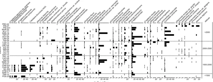
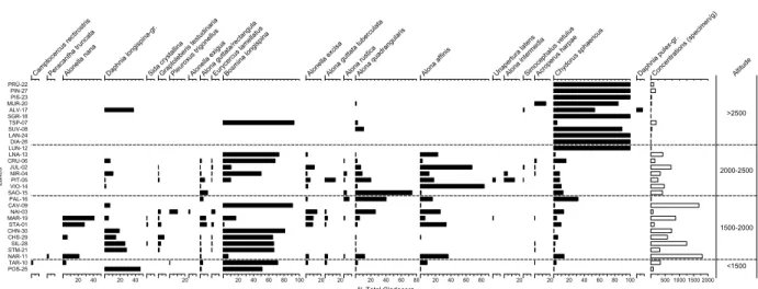
Figure 3. Distribution of most abundant diatoms in surface sediments of the sampled lakes along the altitudinal gradient. The lakes are ab-breviated according to Table 1.
PRÜ-22 PIN-27 PIS-23 MUR-20 ALV-17 SGR-18 TSP-07 SUV-08 LAN-24 DIA-26 LUN-12 LNA-13 CRU-06 JUL-02 NIR-04 PIT-05 VIO-14 SAO-15 PAL-16 CAV-09 NAI-03 MAR-19 STA-01 CHN-30 CHS-29 SIL-28 STM-21 NAR-11 TAR-10 POS-25 Lakes 20 Diam esa Tanyt arsu s II 20 Clad opelm a Thien ema nniel la-ty pe 20 Euk iefferi ella/Tv etenia Micro tendip es Clad otany tars usI Ablabe smyi a Limn oph yes-ty pe Para metrioc nemus /Para phaen oclad ius Crico topus -typ e 20 Orth ocla dius-ty pe Thien ema nnimy ia-type 20 Dicro tendi pes 20 Chiron omus anthra cinus -typ e 20 Proc ladiu s 20 40 Micr opse ctra i nsig nilob us-t ype Para tanyta rsus spp. 20 Tanyt arsu s I 20 Zavrel imyia A 20 Cory non eura s cutell ata-t ype 20 40 60 % Total Chironomids Psect rocl adius (s.s tr.) 20 Hete rotri ssocl adius ma rcid us-typ e 20 40 60 80 Tanyt arsu s luge ns-typ e Para kieffe riella Prot any pus 20 Para tanyta rsus aust riac us-typ e 20 40 60 80 Para cladi us 20 Pseud odiam esa 20 40 60 80 Micr opse ctra r adial is-ty pe 1000 2000 Con cen trati ons (h ead caps ules/g ) 100 200 300 Coun ts Thaum aleida e Chao boru sfla vican s-ty pe 20 Sim uliid ae Altitu de <1500 1000-1500 1500-2000 >2500
Figure 4. Distribution of most abundant chironomids in surface sediments of the sampled lakes along the altitudinal gradient. The lakes are abbreviated according to Table 1.
and alkalinity were low. In contrast, these parameters were more variable at lower elevation. No clear relation-ship between TP, silica, pH, and conductivity and eleva-tion was observed (Fig. 2).
The differences between chemical properties of sur-face waters (1m; epilimnion) and bottom waters (sam-pled a few meters above sediment surface; hypolimnion) are negligible for several chemical variables (i.e., pH, alkalinity, DOC, conductivity). Some lakes showed a distinct thermal stratifi cation (e.g., TSP-7, CAV-9, POS-25, DIA-26 and SIL-28), which particularly affected the TP concentrations, leading to higher TP-concentrations in the bottom water (Table 2). However, three lakes (SGR-18, PRÜ-22 and LAN-24) showed high TP con-centrations in the bottom waters without any distinct thermal stratifi cation. The silica concentrations were in general very similar between surface and bottom waters, except in CAV-9, where a considerably higher value was recorded in the surface water sample (Table 2). The chemical differences in epilimnion and hypolimnion within some lakes illustrate the need for a weighted aver-age approach (see methods) to obtain an appropriate value for each chemical parameter in each lake.
In contrast to TP-concentrations, the measured
TN-concentrations were low (<0.5 mg N L–1
) in all lakes
ex-cept CAV-9 (0.6 mg N L–1
), indicating that the lakes could be nitrogen-limited during the sampled period (Maberly et al., 2002; Camacho et al., 2003). Nitrogen concentra-tions in high altitude lakes are generally rather low in Central Europe, but may show considerable seasonal dif-ferences (Müller et al., 1998). This low nitrogen concen-tration in high altitude lakes is a result of relatively low agricultural land-use in their catchment, but is also af-fected by higher runoff in high-elevation catchments due to increasing precipitation (Müller et al., 1998).
an extension of the number of environmental variables from initially 13 to 29 (Table 1). All 29 environmental variables were initially included in the partial CCAs. The percentage variance explained by each variable was cal-culated (Table 2) and the statistical signifi cance assessed by Monte Carlo permutation tests involving 999 unre-stricted permutations (ter Braak, 1990; Lotter et al., 1997). Subsequently, the environmental data set was re-duced to the most powerful variables explaining the high-est amount of variance in the three biological data sets (Table 2), i.e. July T, LOI, log-Depth, Water T, log1m-Conductivity, 1m-pH, DOC, TP, logWA-alkalinity and WA-Si.
The reduced environmental data set including ten variables and the biological data set including all 30 lakes were used in CCA (Fig. 7). In addition to this direct
gra-dient analysis, we applied a TWINSPAN classifi cation (Hill,
1979) with two division levels to all biological data sets, which resulted in four groups of lakes for each biological data set.
Results
Environmental data and water chemistry
Several environmental variables refl ecting lake water chemistry and lake physical properties are related to cli-matic parameters such as summer and winter tempera-tures, which in the Alps are closely correlated to eleva-tion (Schär et al., 1998) (Table 1). As expected, the measured water temperatures decreased with increasing altitude (Fig. 2), in agreement with a previous survey of the relationship between air and water temperature in the northern Swiss Alps (Livingstone et al., 1999). DOC, LOI, and alkalinity also show a clear relationship with altitude. In high-elevation lakes, values for DOC, LOI
PRÜ-22 PIN-27 PIS-23 MUR-20 ALV-17 SGR-18 TSP-07 SUV-08 LAN-24 DIA-26 LUN-12 LNA-13 CRU-06 JUL-02 NIR-04 PIT-05 VIO-14 SAO-15 PAL-16 CAV-09 NAI-03 MAR-19 STA-01 CHN-30 CHS-29 SIL-28 STM-21 NAR-11 TAR-10 POS-25 Lakes Camp toce rcus recti rostri s Pera canth a tru ncata 20 40 Alon ella nana 20 40 Daphni a long ispin a-gr. Sida crys tallina Grap toleb eris t estud inaria 20 Pleu roxus trigo nellu s Alon ella e xigua Alon a gut tata /rect angul a Eury cerc us lam ellat us 20 40 60 80 100 Bosm ina lon gispi na 20 Alon ella e xcisa 20 Alon a gut tata tube rcula ta Alon a rus tica 20 40 60 80 % Total Cladocera Alon a quad rang ulari s 20 40 60 80 Alon a affi nis Unaper tura late ns 20 Alon a inte rmed ia Sim oce phalu s ve tulu s 20 Acro peru s ha rpae 20 40 60 80 100 Chydor us sp haer icus Daphni a p ule x-gr. 500 1000 1500 2000 Concen tratio ns (s pecim en/g ) Altit ude >2500 2000-2500 1500-2000 <1500
Figure 5. Distribution of most abundant Cladocera in surface sediments of the sampled lakes along the altitudinal gradient. The lakes are abbreviated according to Table 1.
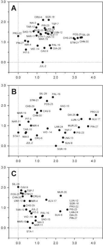
A DCA of all taxa present in at least 3 lakes revealed a compositional gradient of 3.39 standard deviations units along the fi rst axis, indicating that unimodal-based numerical methods are appropriate to analyse the data. The fi rst DCA axis showed a relatively high eigenvalue
(λ = 0.49) and separated the fi ve lakes located at lower
elevations from the rest of the lakes, whereas the second
DCA axis was considerably weaker (λ = 0.17) and did
not show a clear separation of the sampled lakes (Fig. 6A). We calculated a series of partial CCAs using one single constraining environmental variable at a time. For the full lake-set, water depth was identifi ed as the strong-est variable explaining 12.6 % of the variance within the diatom data set (Table 2). Other statistically signifi cant environmental variables were lake-water pH (8.2 %) sili-ca (7.9 %), altitude (7.8 %), alkalinity (7.4 %), mean July
Diatoms
A total of 202 diatom taxa were recorded in the surface sediments of the 30 sampled lakes. The distribution of the most abundant taxa is presented along the altitudinal gra-dient (Fig. 3). Some taxa (e.g., Cyclotella comensis) show distinct abundance patterns in relation to elevation and climate related variables, whereas others (e.g.,
Achnanthes minutissima, Fragilaria spp.) do not. Strong
differences in diatom assemblages were recorded be-tween deep (>30 m water depth) and shallow lakes (3– 15 m). In shallow lakes, surface sediments were domi-nated by periphytic diatoms, whereas in the deeper lakes located at the bottom of the valleys (STM-21, POS-25, SIL-28, CHS-29, CHN-30), planktonic taxa such as
Cy-clotella cyclopuncta, Asterionella formosa and Tabellar-ia fl occulosa dominated the assemblages.
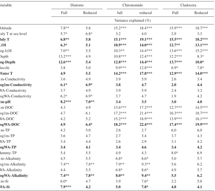
Table 2. Percentage variance explained by each environmental variable in constrained correspondence analyses (CCA) using one single environmental variable at a time. The signifi cance is indicated based on 999 unrestricted Monte Carlo permutations (p < 0.05*, p < 0.01**, p < 0.001***). The full data set includes all 30 lakes; for the reduced data set the deep lakes (i.e., STM-21, POS-25, SIL-28, CHS-29, and CHN-30) were excluded. Bold displayed variables are used for CCA (Fig. 7).
Variable Diatoms Chironomids Cladocera
Full Reduced full reduced Full Reduced
Variance explained (%)
Altitude 7.8** 5.8 15.2*** 18.4*** 15.9*** 18.7***
July T at sea level 5.7* 6.8* 3.2 4.0 2.9 3.3
July T 6.8** 5.8 15.1*** 19.1*** 15.5*** 18.2*** LOI 6.3* 5.1 10.9*** 14.0*** 12.7** 13.1*** log-LOI 7.0** 5.5 10.3** 14.4*** 13.6*** 15.2*** Depth 13.2*** 4.9 10.8*** 12.4*** 12.2*** 8.3* log-Depth 12.6*** 5.4 12.8*** 14.4*** 13.7*** 10.0* Secchi 3.8 5.0 9.9*** 12.8*** 6.9* 7.8* Water T 4.9 5.5 14.2*** 17.8*** 12.9*** 14.0*** 1m-Conductivity 3.6 4.9 3.9 5.9 2.6 3.4 log1m-Conductivity 6.1* 6.9* 3.8 4.7 2.0 4.4 WA-Conductivity 3.7 4.9 3.9 5.9 2.4 3.2 logWA-Conductivity 6.2* 6.9* 3.7 4.7 1.9 4.2 1m-pH 8.2*** 7.0** 3.4 3.5 3.0 4.0 1m-DOC 4.3 4.9 13.6*** 17.2*** 12.7*** 14.5*** log1m-DOC 4.7 6.1 17.2*** 21.4*** 16.3*** 18.7*** WA-DOC 4.2 5.2 15.2*** 18.9*** 13.9*** 16.1*** logWA-DOC 4.9 6.4* 18.2*** 22.4*** 17.4*** 19.9*** 1m-TP 4.2 5.0 2.6 2.7 6.0 6.0 log1m-TP 3.6 4.7 2.7 3.4 3.7 4.3 WA-TP 3.4 4.4 2.6 2.9 3.1 4.2 logWA-TP 3.4 4.1 3.4 4.6 3.4 4.2 dummy-TP 5.4 5.5 4.9 4.3 8.0* 6.9 1m-Alkalinity 4.5 5.5 6.8* 8.6* 5.0 5.7 log1m-Alkalinity 7.4** 7.8** 7.9** 9.3** 5.6 6.2 WA-Alkalinity 4.4 5.5 6.8* 8.6* 4.9 5.7 logWA-Alkalinity 7.4** 7.8** 8.0** 9.4** 5.5 6.2 1m-Si 6.0* 4.7 3.9 7.6* 2.2 5.0 WA-Si 7.9*** 4.2 5.0 7.8* 4.8 4.1
air temperature (6.8 %), LOI (6.3 %) and conductivity (6.1 %). After excluding the fi ve deepest lakes from the data set (STM-21, POS-25, SIL-28, CHS-29, and CHN-30), the explanatory power of lake depth decreased con-siderably and explained only 5.4 % (statistically not sig-nifi cant) of the variance (Table 2). Based on the partial CCA, the set of environmental variables was reduced, by selecting for each parameter the numerical treatment (untransformed/log-transformed, 1 m measurement/WA of measurements) which explained the highest amount of variance in the diatom data set (Table 2).
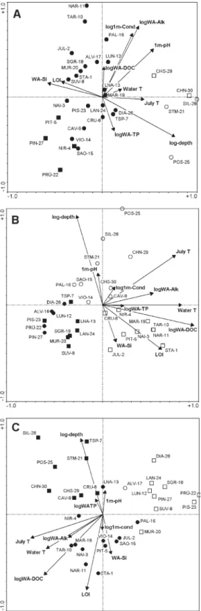
The relationship between the reduced set of environ-mental variables and the diatom distribution was assessed by means of CCA. Lake depth was the strongest environ-mental variable associated with CCA-axis 1 (eigenvalue λ = 0.45) (Fig. 7A), which was negatively correlated with LOI of surface sediment and the silica content of
lake-water (Fig. 7A). The second axis (λ = 0.17) is mainly
related to water chemistry variables, such as conductivity, alkalinity, lake-water pH, and TP. The CCA biplot illus-trates the secondary gradient within the diatom data set, and suggests that both physical (e.g., lake depth, climate, LOI) and chemical (e.g., alkalinity, conductivity, pH, TP) variables have a strong infl uence on diatom distribution patterns.
The diatom classifi cation based on TWINSPAN
separat-ed at the fi rst level the fi ve deep lower-elevation lakes (STM-21, POS-25, SIL-28, CHS-29, CHN-30) from the other samples, mainly because these deep lakes all con-tained the planktonic diatom species Cyclostephanos
in-visitatus (Fig. 7A). At the second level of separation, the
remaining 25 lake-set was split based on water chemistry conditions. One group contained four lakes with rela-tively low lake-water pH (NIR-4, PIT-5, PRÜ-22, PIN-27), where the diatom species Achnanthes scotica and
Achnanthes subatomoides were found. In the large
re-maining lake-subset (n = 21), relatively high pH values were recorded, and diatom assemblages contained spe-cies such as Amphora libyca, Cymbella minuta,
Den-ticula tenuis and Cyclotella comensis. The second
divi-sion within the fi ve deep lakes grouped the two samples from the interconnected lake-basins of Lej da Champfèr (CHN-29, CHS-30) together, based on the occurrence of
Fragilaria robusta. Overall, the TWINSPAN classifi cation
supported the results obtained by ordination methods. Lake depth seems to be the major environmental gradient explaining variations in the diatom fl ora. The secondary gradient seems to be related mainly to water chemistry (pH) and climate (July T).
Chironomids
A total of 62 different chironomid taxa were identifi ed in the surfi cial sediments of the sampled lakes. The chirono-mid assemblages show distinct changes with elevation (Fig. 4). Taxa such as Eukiefferiella/Tvetenia,
Microten-Figure 6. Detrended Correspondence Analysis (DCA) plot includ-ing site scores for (A) diatoms, (B) chironomids and (C) Cladocera. Seven lakes in panel (C) have identical scores due to a uniform fauna.
dipes, and Thienemannimyia-type are found
predomi-nantly in lakes below 2000 m a.s.l. A strong shift in assem-blage composition is apparent at ca. 2300 m a.s.l. A number of common chironomid taxa such as Micropsectra
are largely restricted to lakes below this elevation, and are replaced by taxa such as Paracladius, Pseudodiamesa, and
Micropsectra radialis-type in high-altitude lakes. Only a
few chironomid taxa occur over the entire altitudinal gra-dient, e.g. Corynoneura scutellata-type,
Heterotrissocla-dius marcidus-type or Tanytarsus lugens-type.
A DCA of the chironomid assemblages indicates a gradient length of 4.14 SD units along the fi rst axis (Fig. 6B), therefore indicating that unimodal based numerical methods are appropriate. The fi rst axis separates high-altitude lakes such as PRÜ-22, ALV-17 and PIN 27 from lakes at lower elevations (e.g. STA-1, NAR-11, MAR-19) and is signifi cantly stronger than the second
DCA-axis (λ1 = 0.62, λ2 = 0.22). The second axis seems to be
largely separating deep lakes (e.g. STM-21, SIL-28, POS-25) from the remainder.
Partial CCAs of the full 30-lake data set using a single constraining variable indicate that DOC is the strongest environmental variable explaining 18.2 % of the total variance in the chironomid assemblages (Table 2), close-ly followed by Juclose-ly air temperature (15.1 %) and water temperature (14.2 %). Additional statistically signifi cant variables were maximum water depth (12.2 %), LOI (10.9 %), and conductivity (8.0 %). If the fi ve deep, low-elevation lakes were excluded from the analysis all these parameters explained a distinctly higher proportion of variance in the chironomid assemblages, and the silica concentration became a statistically signifi cant variable (Table 2).
The number of environmental parameters was re-duced by selecting the weighting scheme for the water samples and the transformation that explained the most variance in the partial CCAs (Table 2). A CCA calculated using this reduced environmental data set and the chi-ronomid assemblages of all 30 lakes resulted in a fi rst
CCA axis (λ1 = 0.54) separating high altitude lakes from
lakes at lower elevation (Fig. 7B) and hence also closely related to water temperature, July air temperature and
DOC. The second axis (λ2 = 0.36) separates the deep,
low-altitude lakes from the remaining samples.
At the fi rst level of division, TWINSPAN of the
chirono-mid assemblages splits the 30-lake dataset into two groups of similar size. The fi rst group is characterized by the presence of Micropsectra radialis-type and at least moderate abundances (>2 %) of Paracladius, and con-tains 12 high-altitude lakes (2450–2815 m a.s.l.) with
very low DOC concentrations (0.4–0.9 mg C L–1
). The second group of 18 lakes is typically characterized by
Micropsectra insignilobus-type and includes lakes at
lower altitudes (960–2310 m a.s.l.) with higher DOC
lev-els (0.55–4.61 mg C L–1
). At the second level of division the high altitude lakes are split into a group of seven lakes characterized by the presence of Corynoneura scutellata-type and a group of fi ve lakes characterized by high abundances (>5 %) of Pseudodiamesa, with no clear
dif-Figure 7. Canonical Correspondence Analysis (CCA) ordination biplot with site scores and major environmental variables (see Table 2) for (A) diatoms (B) chironomids and (C) Cladocera. Lake sym-bols are chosen according to TWINSPAN divisions. The fi rst division
separated open from full symbols, the second divisions separated circles from squares.
ferentiation of the two groups in relation to the measured environmental variables. The second division of the lower altitude lakes results in a group of deeper (13–85 m maximum depth), colder lakes (7–15 °C surface water temperature) with lower DOC concentrations (0.6–1.9 mg
C L–1
) and a group of shallower (4–11 m), warmer lakes (12–23 °C water temperature) with somewhat elevated
DOC concentrations (1.1–4.6 mg C L–1
). The group of deeper lakes is characterized by abundances >2 % of
Or-thocladius-type and the shallower lakes by the presence
of Procladius. TWINSPAN confi rms the results of the CCA
by indicating that the chironomid assemblages have the strongest relationship with parameters refl ecting climate and elevation (July air temperature, altitude, DOC), whereas a clear relationship between chironomid assem-blages and lake depth is apparent in lower altitude lakes.
Cladocera
A total of 22 cladoceran taxa were identifi ed in the sam-pled lakes. As in the other two indicator groups the ana-lysed subfossil assemblages show a distinct change and decrease with altitude (Fig. 5). High-elevation lakes typi-cally feature a high abundance of Chydorus sphaericus remains in their surface sediments and a very low diver-sity of cladoceran assemblages. Lakes below ca. 2500 m a.s.l. are characterized by more diverse cladoceran assem-blages including taxa typical for littoral habitats, such as the chydorids Alona quadrangularis, Alona affi nis, and planktonic taxa such as Bosmina longispina and Daphnia
longispina-group. Of the identifi ed cladocerans only a
few are restricted to lakes at lower elevations and of these only Alonella nana occurs in more than one lake. A dis-tinctly lower cladoceran concentration was found in high altitude lakes dominated by chydorids (Fig. 5).
A DCA with the 30-lake dataset reveals a fi rst axis with a gradient length of 2.62 standard deviation units, indicating that unimodal-based numerical methods are appropriate for further analysis. The eigenvalue of the
fi rst DCA axis (λ1 = 0.55) is more than three times higher
than for the second (λ2 = 0.17). The fi rst DCA axis
sepa-rates high-altitude lakes with a high proportion of
Chy-dorus sphaericus from the remaining samples, whereas
the second axis largely separates samples based on the proportion of the planktonic taxa Daphnia longispina-gr. and Bosmina longispina.
Partial CCAs of the full 30-lake data set indicate that DOC explains the highest amount of variance in the cladoceran assemblages (17.4 %), closely followed by altitude (15.9 %), July T (15.5 %), water T (12.9 %) and LOI (12.7 %) (Table 2). All of these environmental vari-ables are signifi cant if assessed by a Monte Carlo permu-tation test. If the deep, low-elevation lakes are eliminated from the analyses the explanatory power of all of these parameters except lake depth shows a distinct increase (Table 2).
A CCA calculated with a reduced environmental da-taset (i.e. with a single value per environmental variable)
produces a fi rst CCA axis (λ1 = 0.46) strongly related to
July T, water T, and partially to DOC (Fig. 7C). This axis separates high altitude C. sphaericus-dominated lakes
from others. The second axis (λ2 = 0.34) is strongly
re-lated to maximum water depth and LOI, partially rere-lated to DOC, and separates the deep, low-elevation lakes and TSP-7 from the remaining lower altitude sites.
The fi rst division of a TWINSPAN classifi cation of
cladoceran assemblages separates 10 high-elevation lakes (>2484 m a.s.l.) from the remaining samples. These lakes are characterized by a high relative abundances (>40 %) of C. sphaericus and low DOC concentrations
(0.4–0.8 mg C L–1
). A single lake (ALV-17) is separated from this group at the second level of division based on the presence of Simocephulus vetulus. The second fi rst division group encompasses lakes over a range of alti-tudes (962–2616 m a.s.l.) with higher DOC
concentra-tions (0.6–5.5 mg C L–1
). At the second-level of TWINSPAN
division this group is split into eight comparatively deeper lakes (max. lake depth 11–85 m) and 12 compara-tively shallower lakes (3.5–20 m) based on the occur-rence of high abundances of B. longispina (>20 %) in the deeper lakes and of the presence of Allonella excisa in the shallower lakes.
Discussion
Biological subfossils in lake sediments contain valuable information about climatic and environmental conditions prevailing during the lifetime of those organisms. How-ever, to interpret subfossil diatom, chironomid and cladoceran assemblages, detailed ecological knowledge about distribution, optima and tolerance of these biota is required. Unfortunately, such information is still frag-mentary (Lotter et al., 1997) and often restricted to local calibration data sets encompassing lakes from a limited geographical area. In the Alps, calibration sets are avail-able for diatoms from the northern and southern Swiss Alps (Lotter et al., 1997; Lotter et al., 1998), the Austrian Alps (Wunsam et al., 1995; Schmidt et al., 2004) and the Italian Alps (Marchetto and Schmidt, 1993). For chirono-mids and cladocerans a surface sediment data set from the northern and southern Swiss Alps has been developed (Lotter et al., 1997; Lotter et al., 1998; Heiri et al., 2003). However, information on the distribution of subfossil di-atoms, chironomids and cladocerans in the surface sedi-ments of lakes from the Central Swiss Alps is still lack-ing. Due to bedrock geology of the catchment of these lakes, the buffering capacity of their waters tends to be low. Consequently, different water chemistry conditions (with respect to, e.g., pH, conductivity, DOC) than in the northern and southern Alps can be expected. Therefore, it
is questionable whether aquatic biota show the same dis-tribution patterns in relation to morphometric, physical and chemical parameters in central Alpine lakes as in hardwater lakes on calcareous bedrock.
The lakes in the Engadine area have been selected to encompass a large altitudinal gradient and include those from high alpine vegetation zones, across the treeline ecotone, to subalpine coniferous forests. In our study lakes, the distribution of diatom, chironomid and cladoceran taxa with respect to elevation is similar to that of the northern and southern Swiss Alps (Lotter et al., 1997; Heiri, 2001). High-elevation diatom assemblages are dominated by species previously reported from alpine lakes in the Alps, such as small Fragilaria taxa (e.g., F.
pinnata, F. pseudoconstruens, F. brevistriata) and Achnanthes minutissima (Fig. 3). At lower altitudes these
species are replaced by planktonic taxa more typical of deep lakes, such as Cyclotella cyclopuncta, Asterionella
formosa, and Tabellaria fl occulosa. Chironomid
assem-blages at high altitudes are dominated by cold steno-thermous taxa, e.g., Micropsectra radialis-type and
Pseudodiamesa (Fig. 4). These taxa are replaced in
warmer, lower elevation lakes by chironomids with a broader altitudinal distribution in the Alps, such as
Tany-tarsus lugens-type and Psectrocladius sordidellus-type,
or in the warmest lakes by taxa such as Micropsectra
in-signilobus-type, Dicrotendipes, Ablabesmyia, Procladius
and Cladopelma. Similar to the northern and southern Alps, high altitude cladoceran assemblages show a very low diversity and often contain Chydorus sphaericus as the only cladoceran species (Fig. 5). At elevations below ca. 2500 m a.s.l. other chydorids become more abundant and planktonic cladocerans such as Bosmina longispina and Daphnia longispina-group can form a large propor-tion of the cladoceran assemblages in the sediments.
Considering the large altitudinal range of our study lakes, it is not unexpected that altitude and correlated environmental parameters such as July T, water T, DOC, and LOI explained a high proportion of variance in the biological proxy data sets (Table 2). This fi nding is in agreement with previously published surface sediment data sets from the northern and southern Swiss Alps,
where summer temperature explained 6.3 %, 6.3 %,
21.4 % and 9.5 % of the variance in subfossil diatom, benthic cladoceran, planktonic cladoceran and chirono-mid assemblages, respectively (Lotter et al., 1997). Simi-larly, summer air or water temperature has been identi-fi ed as important environmental factors in subarctic lakes of northern Europe for diatom (Weckström et al., 1997; Rosén et al., 2000; Bigler and Hall, 2002), cladoceran (Korhola et al., 2000) and chironomid assemblages (Olander et al., 1999; Korhola et al., 2000; Brooks and Birks, 2001; Larocque et al., 2001). Diatoms and cladocerans are not directly exposed to air temperatures during their life-cycle and chironomids only during their
very short adult stage (days to several weeks at most, Oliver, 1971).
It may therefore seem unexpected that July air tem-perature explains more variance in our subfossil assem-blages than the water temperature measurements taken during fi eld work. However, since water temperature can fl uctuate signifi cantly both within the diurnal cycle as well as within a given month, single spot measurements provide only a poor approximation of monthly mean wa-ter temperature values (Livingstone et al., 1999). This may explain the strong relationship between assemblages of all three organism-groups and mean July air tempera-ture in our data set.
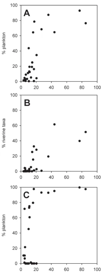
The sampled lakes in the Engadine range from 3.5 to 85 m in maximum depth. Water depth explains a signifi -cant proportion of variance in subfossil assemblages of all three studied organism-groups (Table 2). It has been shown that the proportion of benthic and littoral diatom taxa in sediments from a large, deep lake (Lage Mag-giore, N. Italy) in the southern Alps is low (Marchetto et al., 2004), and similarly, diatom assemblages in deep Engadine lakes (>30 m) consist predominantly of plank-tonic taxa (Fig. 8A). Lake depth affects diatom assem-blage composition mainly through habitat properties and substrate availability (Lotter et al., 2000). Therefore, lake depth is an important explanatory variable for diatom as-semblages in surfi cial lake sediments from the northern and southern Swiss Alps (Lotter et al., 1997), Scandina-via (Bigler et al., 2002) and Alaska (Gregory-Eaves et al., 1999).
Subfossil cladoceran assemblages include both planktonic and benthic taxa. True planktonic taxa in the studied Engadine lakes are Daphnia longispina-group,
D. pulex-group, and Bosmina longispina. Chydorus sphaericus can become planktonic during phases of high
productivity (Frey 1988). However, in the meso- and oli-gotrophic lakes studied during this survey this species, like other chydorid species, most likely forms part of the meiobenthos. In the Engadine, B. longispina is common in lakes below ca. 2500 m a.s.l. and present in a single high altitude lake (TSP-07; Fig. 5). The abundance of this taxon shows no clear relationship with water depth. D.
pulex-group remains have been found in a single
high-altitude lake (ALV-17). In contrast to B. longispina, the abundance of D. longispina-group remains shows a clear relationship with lake depth. With a single exception (ALV-17), high percentages (>18 %) of D. longispina-group are restricted to lakes with a water depth of 36 m or more. The ratio between truly planktonic species and the remaining cladocerans is strongly related to water depth (Fig. 8C), with deeper lakes (>20 m depth) featuring very high percentages of planktonic cladocerans. In shallower lakes a clear relationship between the proportion of planktonic species and water depth is apparent in lakes where Daphnia or Bosmina are present. However, in a
number of shallow lakes true planktonic taxa are absent from the cladoceran assemblages. The distribution of planktonic cladocerans in surface sediments is in agree-ment with other studies which indicate a strong relation-ship between the proportion of planktonic cladocerans in fossil assemblages and lake depth (e.g., Frey, 1988; Ko-rhola et al., 2000; Jeppesen et al., 2001). Planktonic cladocerans in alpine lakes are also strongly affected by the presence of fi sh. For example, Manca and Armiraglio (2002) report that Daphnia remains are largely absent in alpine lakes in northern Italy where fi sh had been regu-larly introduced. Comprehensive data on the presence of fi sh are not available for lakes in the Engadine region, but introduction of salmonids is common practice in lakes in the Swiss Alps (e.g., Barbieri et al., 1999). Therefore, the absence of planktonic cladocerans in many of the shal-lower lakes in our data set may be related to fi sh preda-tion.
In contrast to cladocerans and diatoms, chironomids do not include true planktonic taxa, although the fi rst in-star larvae of some lacustrine species temporarily enter the water column for dispersal. Nevertheless, a statisti-cally signifi cant relationship between chironomid assem-blages and water depth has been observed in the Enga-dine lakes (Table 2). Studies of the distribution of living chironomid larvae indicate that a number of species show a preference for either deep lakes and hypolimnetic envi-ronments, or shallower lakes and littoral environments (e.g., Brundin, 1949; Gerstmeier, 1989; Rieradevall et al., 1999). Surprisingly, subfossil chironomid assemblages in the deepest lakes in our data set show an increased rela-tive abundance of taxa typical of stream habitats rather than of taxa typical for deep lakes. The percentage of chironomids typical of running water ranges between 6 and 27 % in lakes shallower than 6 m but rises to 14 to 85 % in lakes deeper than 15 m (Fig. 8B). Furthermore, deeper lakes such as STM-21, SIL-28, CHN-30, CAV-9 and PAL-16 contain a high proportion of subfossils be-longing to Simuliidae and Thaumaleidae, aquatic insects restricted to running water habitats (Currie and Walker 1992; Wagner 1997) (Fig. 4). In general, the chironomid assemblages in the deepest parts of lake basins are com-posed of species living in the lake center, and those trans-ported into deeper parts originating from the margins of the lake and its tributaries (Hofmann, 1971; Frey, 1988; Heiri, 2004). Furthermore, low oxygen conditions in the bottom waters, as reported from at least one lake in our data set (STM-21, Züllig, 1995), and food limitation in the hypolimnion can become an important factor restrict-ing the occurrence of benthic animals (Wetzel, 2001). Thus, the high proportion of running water chironomid remains in the deepest study lakes could be explained by a reduced abundance of chironomid larvae living in the hypolimnion in combination with a preferential deposi-tion of running water chironomid remains. Available
evi-Figure 8. Percentages of planktonic diatoms (A), running water chironomids (B) and planktonic cladocerans (C) in subfossil assem-blages in the surface sediments of the 30 study lakes.
dence therefore indicates that the strong relationship be-tween lake depth and chironomid assemblages in our data set is infl uenced to a large extent by taphonomic processes (i.e. transport of chironomid remains from stream habitats to the lake center).
Diatom assemblages in our data set show a signifi cant relationship with lake-water pH, alkalinity and silica. Again, these chemical variables have previously been reported as infl uencing subfossil assemblage composi-tion, for example in the northern and southern Swiss Alps (Lotter et al., 1997; Lotter et al., 1998), the Austrian Alps (Wunsam et al., 1995; Schmidt et al., 2004), or in Scan-dinavia (Weckström et al., 1997; Rosén et al., 2000; Bigler et al., 2002). Even though lake-water pH (and al-kalinity) is probably the strongest variable controlling diatom assemblage composition by affecting many chemical and biochemical processes, there is still no de-tailed physiological understanding on how pH infl uences competition between diatom taxa (Battarbee et al., 2001). Silica is important both in regulating the size of phyto-plankton crop and the species composition, but usually phosphorus and nitrogen are the most important nutrients regulating diatom assemblage composition (Battarbee et al., 2001). In our data set, the phosphorus gradient is rather short and nitrogen concentrations are (except in CAV-09) below detection limit, thus giving silica a more important role in explaining the diatom assemblage com-position in the numerical analysis.
For chironomids and cladocerans in the Alpine re-gion, the high explanatory power of DOC is, in contrast to temperature or lake depth, unexpected. In Scandinavi-an humic lakes, where the concentration of DOC is often related to altitude (Karlsson et al., 2001; Larocque et al., 2001), DOC has been reported as a major environmental variable infl uencing chironomid assemblage composi-tion. However, in the Alpine region DOC concentrations are generally substantially lower than in Scandinavian brownwater lakes. Furthermore, chironomid assemblages in our data set are not dominated by taxa typical for hu-mic lakes such as Zalutschia zalutschicola, or
Heterot-anytarsus apicalis. The zooplankton of humic lakes
typi-cally features a high abundance of Chaoborus fl avicans (Diptera: Chaoboridae). However, only a single C. fl
avi-cans-type mandible was found in one of the Engadine
lakes with comparatively high DOC concentrations (NAR-11; Fig. 4). In lakes in the northern and southern Swiss Alps, DOC concentrations explain only 4.8 %, 15.6 % and 6.9 % of the variance in subfossil benthic cladoceran, planktonic cladoceran and chironomid as-semblages, respectively (Lotter et al., 1997). This con-trasts with 17.4–22.4 % of the total variance explained by DOC in the cladoceran and chironomid assemblages ana-lysed in the Engadine area (Table 2). In our study lakes DOC is highly negatively correlated with altitude (r = – 0.69) in lakes higher than 1400 m a.s.l. This relationship
is stronger than the correlation between DOC and alti-tude in lakes in the northern and southern Alps in a simi-lar altitudinal range (r = –0.38) (Lotter et al., 1998). It is therefore possible that the strong relationship between chironomid and cladoceran assemblages and DOC in the Engadine lakes is actually a consequence of the strong infl uence of temperature on the studied lake ecosystems rather than an effect of the different DOC concentrations. However, lakes in the Engadine feature distinctly higher DOC values at the lower end of this altitudinal range than lakes on calcareous bedrock in the northern and southern Alps (Fig. 9). A number of key parameters for lake eco-systems such as light penetration and oxygen concentra-tions can be strongly infl uenced by DOC concentraconcentra-tions, leading to distinct zoobenthos and zooplankton assem-blages in humic lakes (e.g., Brundin, 1949; Nyman et al., 2005). It may therefore also be possible that the elevated DOC concentrations in some of the studied lakes in the Engadine area had a distinct infl uence on chironomid and cladocerans assemblages independent of temperature.
LOI also explains a signifi cant proportion of the vari-ance in the chironomid and cladoceran assemblages (Ta-ble 2). The organic matter content of sediments, usually assessed as LOI, has been reported as a strong explana-tory variable in surface sediment cladoceran and chirono-mid assemblages in Fennoscandia (Korhola et al., 2000; Larocque et al. 2001). However, in these data sets, as in the Engadine lakes, LOI is correlated with summer tem-perature. Next to the correlation with summer tempera-ture (r = 0.35) LOI also shows a negative correlation with water depth in our study lakes (r = –0.39), with the coolest and deepest lakes containing sediments with a very low organic matter content and warm, shallow lakes featuring a wide range of LOI values (Table 1). Further-more, LOI is highly correlated with DOC (r = 0.77). Since at least chironomid larvae can inhabit lake sedi-ments themselves and a number of chironomids and cladocerans are detritus feeders (Pinder, 1986; Korhola et al., 2001) the organic matter content of lake sediments may have a distinct impact on chironomid and cladoceran populations. However, for both organism-groups summer temperature, DOC, and water depth explain a higher pro-portion of the variance. Therefore, the apparent relation-ship between chironomid and cladoceran assemblages and LOI may be infl uenced to a considerable extent by the effects of temperature, DOC, and water depth.
In contrast to a number of studies relating the distri-bution of surface sediment assemblages of diatoms, chi-ronomids, and cladocerans to lake nutrient conditions (e.g., Bennion et al., 1996; Brodersen et al., 1998; Lotter et al., 1998; Brooks et al., 2001), TP values in the studied lakes did not explain a signifi cant proportion of variance for any of the studied organisms. This is likely a conse-quence of the comparatively short phosphorus gradient encompassed by our study lakes, which do not include
strongly eutrophic and hypertrophic lakes. Furthermore, the strong gradients in elevation and lake depth may have further obscured any relationship between the fossil as-semblages and lake nutrient conditions.
Conclusions
We studied the relationship between subfossil diatom, chironomid, and cladoceran assemblages in the surface sediments of 30 lakes in the Engadine area, SE Switzer-land, and major physical and chemical parameters. Our aim was to identify relevant environmental parameters for biota in these lakes in order to compare them with existing calibration data sets on different bedrock or in different geographical regions. Strong, statistically sig-nifi cant relationships have been identifi ed between dia-tom assemblages and water depth, pH, and the silica content of lake water, whereas weaker relationships were observed between diatoms and alkalinity, July air tem-perature, and the organic content of lake sediments. Chi-ronomid and cladoceran assemblages show a strong rela-tionship with parameters correlated with altitude in the Engadine lakes such as the DOC content of lake water, July air temperature, water temperature, and the organic content of lake sediments. Furthermore a strong relation-ship exists with water depth for both organism-groups.
The distribution of diatom, chironomid, and cladocer-an assemblages with altitude is similar in the Engadine region as in the northern and southern Alps, although in the poorly buffered waters of south-eastern Switzerland this relationship may be reinforced by the strong correla-tion between the DOC content of the lakes and elevacorrela-tion. Increasing lake depth is refl ected in diatom and cladocer-an assemblages by a higher proportion of remains
origi-nating from planktonic taxa. In contrast, chironomid as-semblages in the deep Engadine lakes were characterized by high abundances of running water taxa.
The strength of the relationship between the different environmental parameters and the subfossil assemblages indicate that parameters related with altitude and temper-ature exert the strongest infl uence on the composition of subfossil chironomid and cladoceran assemblages in the Engadine area. This suggests that, as in alpine lakes on calcareous bedrock (Lotter et al., 1997; Heiri and Lotter 2005), fossil assemblages of these organisms have con-siderable potential as palaeotemperature indicators. In contrast, the relationship of diatoms to elevation is con-siderably weaker in the Engadine, and assemblages are also strongly infl uenced by water depth and water chem-istry variables such as pH and silica concentrations.
Acknowledgments
We cordially thank P. Bluszcz, C. Casty, U. Heusi, I. Hof-mann, W. HofHof-mann, M. Langmeier, F. Oberli, C. Ohlen-dorf, V. Korinek, T. Kulbe, K. Sarmaja-Korjonen, M. Wehrli, and A. Zwyssig for assistance during fi eldwork, sample preparation, and analysis. The Youth Hostels in St. Moritz and Pontresina, the municipality of Stampa, and the Air Grischa supported us with logistics, trans-ports and sample storage. Meteorological data (Climate Normals 1961–1990) were provided by MeteoSwiss and kindly prepared by D. Steiner. This project was supported by the Swiss National Science Foundation through the NCCR Climate program, and the EU Project EMERGE. OH has been supported by the Nederlandse Organisatie voor Wetenschappelijk Onderzoek (NWO)/Aard – en Levenswetenschappen (ALW) project Holocene winter
precipitation and summer temperatures in the Central Alps: reconstructing long-term NAO indices (Grant Nr.
813.02.006). This is Netherlands Research School of Sedimentary Geology (NSG) publication no 20060201. References
Anderson, N. J. and R. W. Battarbee, 1994. Aquatic community persistence and variability. A palaeolimnological perspective. In: P. S. Giller, A. G. Hildrew and D. Raffaelli (eds.), Aquatic ecology: scale, patterns and processes, Blackwell Scientifi c Publications, London, pp. 233–259.
Ariztegui, D. and J. Dobson, 1996. Magnetic investigations of fram-boidal greigite formation: A record of anthropogenic environ-mental changes in eutrophic Lake St Moritz, Switzerland. The Holocene 6: 235–241.
Ariztegui, D., P. Farrimond and J. A. McKenzie, 1996. Composi-tional variations in sedimentary lacustrine organic matter and their implications for high alpine holocene environmental changes: Lake St Moritz, Switzerland. Organic Geochemistry 24: 453–461.
Barbieri, A., M. Veronesi, M. Simona, S. Malusardi and V. Straškrabová, 1999. Limnological survey in eight high moun-Figure 9. DOC concentrations in lakes in the Engadine region (solid
squares) and in the northern and southern Swiss Alps (open squares; Lotter et al., 1998) plotted versus altitude. Only lakes above 1400 m a.s.l. are shown.