HAL Id: hal-01213803
https://hal.archives-ouvertes.fr/hal-01213803
Submitted on 4 Nov 2015
HAL is a multi-disciplinary open access
archive for the deposit and dissemination of
sci-entific research documents, whether they are
pub-lished or not. The documents may come from
teaching and research institutions in France or
abroad, or from public or private research centers.
L’archive ouverte pluridisciplinaire HAL, est
destinée au dépôt et à la diffusion de documents
scientifiques de niveau recherche, publiés ou non,
émanant des établissements d’enseignement et de
recherche français ou étrangers, des laboratoires
publics ou privés.
The Use of an Array Processor for the Simulation of
X-ray Topographs
Alain Soyer, Yves Epelboin, François Morris
To cite this version:
Alain Soyer, Yves Epelboin, François Morris. The Use of an Array Processor for the Simulation of
X-ray Topographs. Journal of Applied Crystallography, International Union of Crystallography, 1985,
18 (2), pp.85-92. �10.1107/S0021889885009888�. �hal-01213803�
85
J. Appl. Cryst. (1984). 18, 85-92
The Use of an Array Processor for the Simulation of X-ray Topographs
By A. SOYER, Y. EPELBOIN AND E MORRIS
Laboratoire de Mineralogie Cristallographie, associk au C N R S , Universitks P. M. Curie et Paris V I I , 4 place Jussieu, 75230 Paris C E D E X 05, France
(Received 2 April 1984; accepted 19 November 1984)
Abstract
The use of a varying-step algorithm now allows the simulation of traverse topographs and of section topographs taking into account the real width of the incident beam. However, computation time remains a critical factor in practical use. With an array processor it is possible to decrease the computation time signifi- cantly• It is shown that pictures of good quality may be obtained in a reasonable time using local facilities• The influence of various parameters on the accuracy of the simulations is discussed• It is demonstrated that local machines can be more useful, in crystallography, than giant computers often difficult to reach through the network of communications.
Introduction
Simulation is now widely used to understand the contrast of defects in X-ray crystallography. As early as 1967 Balibar & Authier successfully computed the contrast of a dislocation in a section topograph. However, the computation time was too long for any practical use. Improvements in the program and new computers made it possible in 1974 (Epelboin, 1974) where simulation started to be used to understand the contrast of defects. Since then different authors have successfully simulated the contrast of various defects: Ishida, Miyamoto & Kohra (1976) simulated the contrast of a dislocation in a plane-wave experiment; Bedynska, Bubakova & Sourek (1976), Riglet, Sauvage, Petroff & Epelboin (1980) simulated the contrast of dislocations in the Bragg case; Nourtier, Klemen, Taupin, Miltat, Labrune & Epelboin (1979) simulated the contrast of ferromagnetic walls; Capelle, Epelboin & Malgrange (1982) studied the contrast of antiphase boundaries.
Through simulations it has been possible to measure quantitative parameters of various defects but by means of section topographs only. The simula- tion of traverse topographs was impossible because the precision of the numerical algorithm to integrate the Takagi-Taupin (TT) equations (Takagi, 1962, 1969; Taupin, 1964) was not good enough. New algorithms (Petrashen, 1976; Epelboin, 1981)make it now possible (Petrashen, Chukovskii & Shulpina,
1980; Epelboin & Soyer, 1985). However, time remains a critical factor since the simulation of one traverse topograph may need tens of hours using a giant computer such as an IBM 3081!
In this paper we will explain how a small array processor linked to a minicomputer can be used to overcome this difficulty. This was not obvious since T T equations are only partially vectorizable and we had to write special subroutines in assembler language (APAL) for the array processor• Furey, Wang & Sax (1982) have already shown that protein structure refinement can be done using array processors. Our conclusion is that in the future various problems in crystallography may be solved not only with giant and very expensive machines such as a CRAY but also by programming small dedicated machines•
In § I we will briefly recall the principles of numer- ical integration. Then in § II we will explain the main features of the array processor and give some highlights on the flowcharts of the programs• In § III we will discuss the influence of the resolution on the accuracy of the simulations.
I. Principles of the numerical integration
We will only briefly describe the numerical algorithm. Details may be found in other papers (Epelboin & Soyer, 1985; Soyer, 1983) and we will just recall the basic principles.
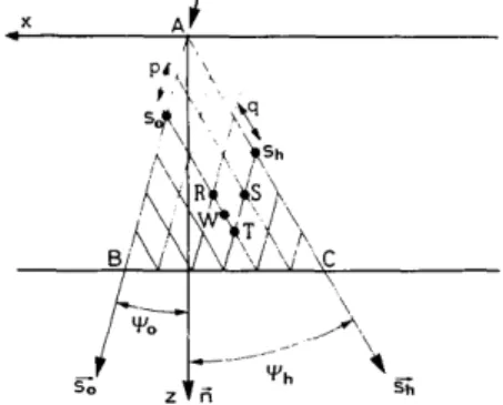
TT equations are a set of partial derivative hyperbo- lic equations (Takagi, 1962, 1969; Taupin, 1964) giving the amplitudes of the refracted and reflected waves D O and Dh at any point inside the Borrmann fan (Fig. 1):
O/OsoDo(r) = _ inkZ Dh(r)
O/•ShDh(r) = -- irckZhDo(r) + 2in[kflh -- 8/~'Shh.U(r)]Dh(r).
(1)
So and Sh are a set of oblique axes parallel to the refracted and reflected directions respectively (Fig. 1).
flh matches the extremities of the wave vectors inside the crystal and is equal to zero in our calculations, Zh
and Z- are the Fourier components of the dielectric
h • • •
susceptlbdlty, h is the reciprocal-lattice vector and u(r) is the local deformation at point r. The equations are written for one state of polarization only.
86 SIMULATION OF X-RAY TOPOGRAPHS These equations are numerically integrated step by
step along the So and Sh directions. Using the half-step derivative method (Authier, Malgrange & Tournarie,
1968) they may be written as:
Oo(So- p,
l o so,
i
\Oh(So, Sh)J
=-d
A B B C, .] IDo(so, sh--q) "LDh(So, Sh - q)_
(2)
p and q are the local steps of integration at point So, sh in the Borrmann fan.
A = - ½ipnkz~ B = --½iqrckZh W = -- ixqc3/C3Sh[h.u(r)]
d = I - W - A B
C~ = I + W; C 2= l - W.
Starting from one point source A along the entrance surface of the crystal (Fig. 1), the amplitudes of the wave fields are computed in all the Borrmann fan
A B C along a set of characteristic lines. Equations (2) show that the amplitudes of the reflected and refracted waves at point T depend on the amplitudes of the waves at points R and S only (Fig. 1). The local deformation of the crystal is computed at point W.
The steps of integration p and q may be fixed through all the integration (Authier, Malgrange & Tournarie, 1968) but the precision of the integration is insufficient to compute traverse topographs or section topographs taking into account the real width of the incident beam. It is necessary to use a varying-step algorithm (Epelboin, 1981, 1983). Its principles are described in Fig. 2. The steps of integration are chosen to follow the oscillations of the amplitudes of the waves (Fig. 2b): they are smaller near the edges of the Borrmann fan, larger in the middle where D o and Dh vary slowly. When a defect intercepts the refracted beam the density of nodes in the network of in- tegration is increased (Fig. 2a). Explanations about the choice of these networks are given by Epelboin (1983).
q x
p~I'\~ J ' \ . "~ q
Fig. 1. Schematic of the numerical calculation.
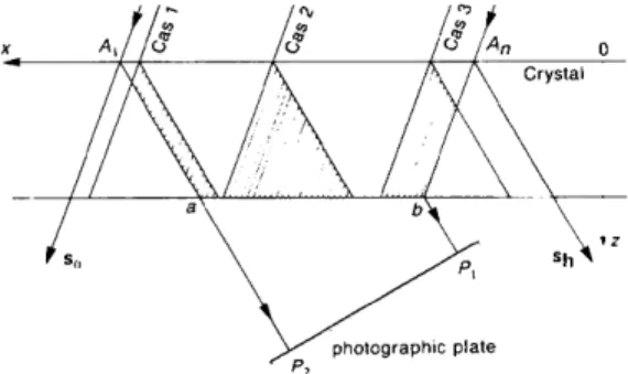
The computation of one integration gives a profile of intensity along the exit surface of the crystal in one plane of incidence. When simulating a section topo- graph, taking into account the real width of the incident beam, the computation is repeated for follow- ing positions of the point source along the entrance surface (Fig. 3). The number of point sources depends on the width of the beam. The same principle applies when simulating a traverse topograph: to compute the intensity along ab on the exit surface of the crystal (Fig. 4) the computation is repeated from O to O' and all the resulting intensities are added together. Since near the edges of the image not all the nodes of the network of integration contribute to the calculation,
x Y" 7?::,2, ~ ' ~ ",~, 2 i',, /, , rSo *z Sh~ (a) x • t S O Vz Sh • (b)
Fig. 2. (a) Network of integration in the areas of the crystal where the direct image exists. (b) Network of integration without refinement for the direct image.
1 2 3 ..' .. / ~
"" ':g ",
L ~
Fig. 3. Principle of the simulation of a section topograph taking the width of the incident beam into account.
A. SOYER, Y. E P E L B O I N A N D E M O R R I S 87 time may be saved by computing the amplitudes of the
waves only in part of the Borrmann fan: near point b only the left part is used as shown in Fig. 5, near point a only the right part is computed. This saves appreciable time especially when the image is not large.
II. Use of an array processor
(a) Principles of programming
An array processor is a computer especially designed for scientific use. The FPS (Floating Point Systems Co.) FPS100 array processor includes three pro- cessors: a floating-point adder, a floating-point multi- plier and an integer arithmetic and logical unit. They can process data in the same cycle in parallel. Their pipe-line structure, the different ways to link them together and to the data and constant memories explain why, when well programmed, an array pro- cessor can achieve a very high speed of calculation: a multiplication is performed in 750 ns; an array of 1000 multiplications using the same operand can be done in 250"5 ItS only. To be efficient a program must take advantage of the pipe-line architecture and of the parallelism to execute the maximum number of opera- tions in the same cycle: in the same cycle one may start an addition and a multiplication and transfer data from/to the memory. The FPS100 is comparable to the FPS120; the main difference is the cycle time: 250 ns instead of 167 ns. I t i / o / /, /,, / ',, i • i " ? i a b
Fig. 4. Principle of the simulation of a traverse topograph.
~S~
a b...
2
photographic plate P2Fig. 5. Principle of the simulation of a traverse topograph; the shaded areas indicate the parts of the Borrman fans that must be taken into account near the edges and in the middle of the image.
The array processor is linked to a host: a BULL MINI6/53 16 bit minicomputer in our case (this machine is comparable in speed to a D E C 11/70). Input and output are done through the host and the programs are compiled in the host. A mathematical library for array calculations is provided with the API00; matrix products, Fourier transforms, signal processing can be done by simple Fortran calls to this library.
Let us assume for simplicity that the steps p and q are the same in all the Borrmann fan as drawn in Fig. 1. Thus the nodes R and S lie along a line parallel to the surface of the crystal. The program can be written in such a way (Authier, Malgrange & Tournarie, 1968) that the amplitudes are computed line by line parallel to the surface of the crystal. The (n + 1)th line (node T) is computed after the calculation of the nth line (nodes
RS)
and from equations (2) it is obvious that this part is vectorizable. It is necessary to store in the computer the values of the reflected and transmitted waves for both lines and 8(n + 1) values for the components of the 2 × 4 matrix at the n nodes.However, some difficulties appear:
To compute the (n + 2)th line it is necessary to replace the values of the amplitudes of the nth line by the values of the amplitudes of the (n + 1)th line. Otherwise all lines should be stored in the central memory of the computer. Thus a complete vectorization would need a very large memory (typically there are more than 105 nodes in the Borrmann fan) to store all the amplitudes and components of the matrix at each node.
Another severe limitation to the vectorization is the problem of the computation of W. It needs a test to avoid an overflow when the node is too near the core of the dislocation.
We may summarize the problem of the vectoriza- tion as follows:
(1) Compute all the components of the 2 × 4 matrix for line n (only partially vectorizable).
(2) Compute line n + 1 (vectorizable).
(3) Transfer the contents of the amplitude arrays for line n + 1 into the arrays for line n (vectorizable).
This process is repeated until the exit surface of the crystal is reached.
O u r analysis shows that 80% of the computation time is used in step l and the Fortran compiler is unable to speed up the calculation when using an array processor. But, when written in assembler lan- guage, a program may take advantage of the archi- tecture of the machine to run all the processors and transfer lines at maximum efficiency. We had to write the program in assembler language (APAL). As a first step we wrote a Fortran version. Then the sensitive part of the program,
i.e.
the integration of TT equa- tions, was written in APAL. The sequence of instruc- tions in the assembler version had to be reordered for a better parallelism. Some operations were performed88 SIMULATION OF X-RAY TOPOGRAPHS
in advance to save cycles each time a processor was not busy. The many registers were used to save intermediate data. No one compiler would be able to reorganize a program as a programmer does! It means that the APAL version, although performing the same calculations as the Fortran version, is logically orga- nized in a complete different way.
(b) Flowchart
Starting from the data of one point source along the entrance surface (point A in Fig. 1) the amplitudes are computed along characteristic lines parallel to So. At the end the intensities along BC are known. This calculation is done in the array processor.
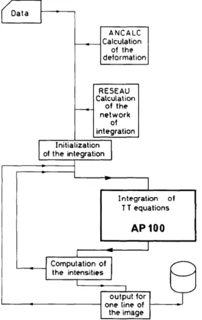
Fig. 6 shows a schematic flowchart for the simula- tion of section topographs (DEF V). When the width of the entrance slit is taken into account the integration is repeated for following positions of point A (Figs. 1 and 3) along the entrance surface and the computed intensities are transferred into the host and added together. Then the result, for one line of the image corresponding to one plane of incidence, is stored on a magnetic device. This is repeated for each line of the image. To save computation time and when maximum
resolution is not required one line of the image over two or three planes of incidence is computed, the missing ones being interpolated.
The computation of a traverse topograph (program
ADELE) is more complicated. The calculation may
need tens of hours and it is not always possible to obtain such a time for one single job or the machine may go down! Thus it was necessary to be able to restart the computation where it had stopped. Fig. 7 is the flowchart for A DELE. Data are read in a separate program I N I T and create a set of save files that are used to start the program itself. Each line of the image (corresponding to one plane of incidence) is computed in the AP100 and then stored on a disk; at the same time the save files are updated so that, in case of need, the computation may restart from the previous line of the image. For safety reasons two save files are alternately updated. To minimize the dialogue between the host and the array processor complete lines of the images are computed in the AP100 and an exchange is initiated only to write on the disk.
The performances of the array-processor versions of
D E F V and ADELE are satisfactory: it is possible to
run these programs faster than using a big machine such as an IBM 370/168 or an Amdhal V7. Table 1
1
ANCALC = Calculation of the deformation RESEAU Calculation of the n e t w o r k of integration Initialization I of the integration D Integration of T T equations APIO0I
I Computation
of J
_~
I the intensities 1 = II output for I one
line of the image
Fig. 6. Flowchart for DEFV. The thick lines indicate the part of the calculation that is performed by the AP100.
Program I N ! T = Initializations Program ADELE I Simulation t " t " Calculation of
r one line of the image
I 4
I output
o, 1 ~ . - ~
L-toutou, o,i
~ t h e s a v e files I
A P I O 0
Fig. 7. Flowchart for ADELE. Initial calculations are performed with program I N I T then the integration is done in a second program ADELE.
A. SOYER, Y. EPELBOIN AND E MORRIS 89 Table 1. Comparison of the times of computation using
different computers
Computer Language Time
Bull MINI6/53 Fortran 77 6 h
with FPS 100 Fortran 77+ APAL 13 min
IBM 370/168 Fortran X 40 min
Amdhal V7 Fortran X 18 rain
Cray I Fortran 77 3 min 46 s
shows the time needed to compute one line of the image in Fig. 8(a) using different computers. This calculation was especially long since the resolution is very high as will be explained in the next section and simulation of traverse topographs may be obtained in a shorter time. This example shows that this small machine programmed in APAL is only three times
(a)
slower than a giant machine such as a CRAY 1 but it must be recalled that vectorized Fortran compilers are not able to vectorize such a program.
Since the result is an image that has to be drawn on a picture system the situation is worse when using the CRAY 1: the results must be shipped back through the telecommunication network, which is not usually fast enough. This is especially true for section topographs where an image is computed in 3 to 15 min using the AP100. The total time needed to use a CRAY 1 and receive the results would always be greater. Only people on the site may obtain faster outputs. Moreover, since most of the computation is done in the array processor only a few resources are needed from the host.
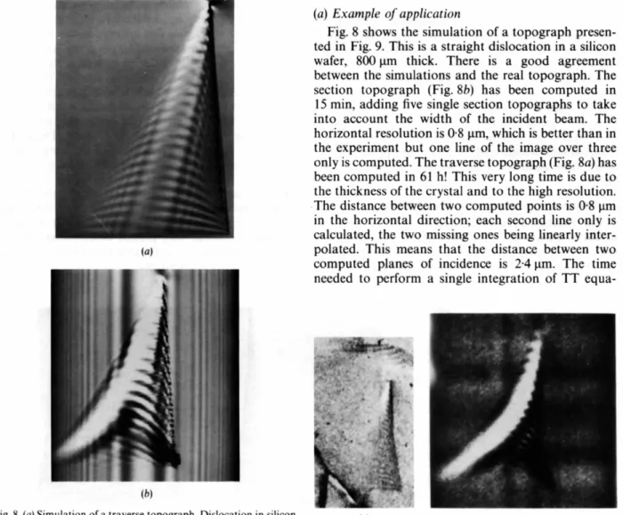
IlL Applications (a) Example of application
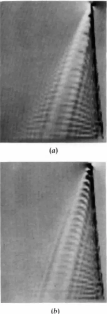
Fig. 8 shows the simulation of a topograph presen- ted in Fig. 9. This is a straight dislocation in a silicon wafer, 800 I~m thick. There is a good agreement between the simulations and the real topograph. The section topograph (Fig. 8b) has been computed in 15 min, adding five single section topographs to take into account the width of the incident beam. The horizontal resolution is 0"8 ~tm, which is better than in the experiment but one line of the image over three only is computed. The traverse topograph (Fig. 8a) has been computed in 61 h! This very long time is due to the thickness of the crystal and to the high resolution. T h e distance between two computed points is 0-8 lam in the horizontal direction; each second line only is calculated, the two missing ones being linearly inter- polated. This means that the distance between two computed planes of incidence is 2-4 ~tm. The time needed to perform a single integration of TT equa-
. .
, ~.~ ~,~ . . •
(b)
Fig. 8. (a) Simulation of a traverse topograph. Dislocation in silicon 800 ~m thick. Mo Kct 220, b-- 1/2 [10I], 400 x 330 I~m. Reso- lution if8 ~tm. Each second line only is computed. Time of computation 61 h. (b) Simulation of the section topograph. Incident slit 17-6 ~tm. Time of computation 15 min.
(a/ (b)
Fig. 9. (a) Experimental traverse topograph corresponding to Fig. 8(a). (b) Experimental section topograph corresponding to Fig. 8(b ).
90 SIMULATION OF X-RAY TOPOGRAPHS tions is proportional to the number of nodes in the
network of integration (Fig. 2), thus roughly propor- tional to the square of the thickness of the crystal. In the traverse topograph one adds single section topo- graphs, translating the source along the entrance surface of the crystal with a step equal to the required horizontal resolution (Epelboin & Soyer, 1985), thus the number of integrations is directly proportional to the resolution in the image. Since this simulation (Fig. 8a) contains 511 x 412 pixels, each line means 790 integrations of TT equations in 171 planes, each integration being computed on 31 250 nodes of the network of integration. Hopefully, as will be explained later, images can be simulated faster.
Some differences may be noticed between the simula- tion and the experiment: fringes are visible in the left part of the simulation that do not appear in the real topograph. This is due to the lower accuracy of the experiment and to the presence of other defects in the vicinity, which locally slightly modify the deformation of the crystal: we always assume a straight dislocation isolated in the crystal. The accuracy of this simulation is good enough to identify the Burgers vector of the dislocation without any doubt (Epelboin & Soyer, 1985).
The images have been drawn on a raster picture system Numelec Pericolor 2000 with 256 different gray levels. An internal transfer function allows the densitometric response of the film to be approximately taken into account. This will be enhanced in the future.
(b) Optimum parameters for image simulation
The preceding example is not very realistic. It would be unwise to simulate traverse topographs over such a long time. This is not true for section topo- graphs where the time of computation is always
reasonable. Since the experimental resolution is never better than 1 lam and quite often of the order of 3 lam, we have investigated which are the most realistic parameters for the practical use of simulation. The answer is not unique since it depends on the object of interest. One must be able to see the details of the structure under study.
Reducing the resolution along a horizontal line does not save any computation time since the number of points where the intensity is calculated along the exit surface of the crystal in one plane of incidence is related to the number of nodes in the network of integration. The pixels along a horizontal line of the image are a sampling of the intensities on the nodes corresponding to the exit surface. The number of nodes cannot be reduced without introducing numer- ical errors. Thus, in the case of section topographs, the interest of a lower resolution is to increase the distance between following planes of incidence decreasing the number of integrations. In the case of traverse topo- graphs it also permits one to reduce the number of elementary section topographs since the sampling of the sources along the entrance surface is equal to the sampling of the pixels along a line of the image (Epelboin & Soyer, 1985). It is also possible to save appreciable time enlarging the distance between fol- lowing planes of incidence and computing additional lines in the image by linear interpolation. Depending on the thickness and orientation of the fringes in the image it might be necessary to compute all the lines of the image or each second one only. When the experi- mental image is known it is theoretically possible to adapt dynamically the distance between integrated lines. However, this is not practical since it would be necessary to make very precise measurements in the image: the position of a defect is never known with an accuracy better than 10 lam.
, ~ ~ : , , :
: ~~
(a) (b) (c)
Fig. 10. (a) Same simulation as in Fig. 8(a). Resolution 1-6 lam. Time of computation 15 h 20 min. (b) Same simulation as in Fig. 8(a). Resolution 2-4 lam. Time of computation 6 h l0 min. (c) Resolution 2.4 lam. One line out of two is computed. Time of computation 11 h 25 min.
A. SOYER, Y. E P E L B O I N AND E MORRIS 91 Fig. 10(a) is the same simulation as in Fig. 8(a) but
the resolution is reduced to 1.6 I~m and one line of the image out of three only is computed, the two missing ones being interpolated. The quality of the image is good and the computing time is reduced to 15 h 20 min. In Fig. 10(b) the data are the same except for the resolution, which is 2.4 pm. Interpolating the missing lines introduces errors: the shape of the horizontal fringes is reversed since the distance be- tween two computed lines is now 7.2 ~tm and this creates an artificial moir6 effect. The computation time is reduced to 6 h and would be satisfactory if the image did not present horizontal features that become wrong. Computing one line out of two (Fig. 10c) with the same resolution gives a good result with a time of 11 h 25 min.
In a first study one is interested in large features of an image only; thus a resolution of 3"2 p.m might be sufficient if one line out of two only is interpolated. Figs. 1 l(a) and (b) show the same dislocation but with two opposite Burgers vectors. The strong white con- trast in Fig. l l(a), near the point where the dislocation intersects the exit surface of the crystal, identifies the
(a)
1
(b)
Fig. 11. (a) Resolution 3.2 pm. Time of computation 5 h 12 min. (b) Same simulation as (a) except b = 1/2 IT10].
Table 2. Time of computation versus resolution and quality of the simulated images
Times are given as ratios of the shortest one, which is 3 h 28 min
Distance between Horizontal computed
resolution lines Time Remarks
0.8 pm 0.8 ~tm 48 Very good but too long 1"6 I.tm 24 Very good but too long
2.4 ~tm 16 Good
1.6 ~tm 1.6 ~tm 12 Good
3.2 I~m 6 Good
4.8 ~tm 4 Good, reasonable time
2.4 I~m 2.4 I~m 5.3 Good
4.8 pm 2.6 Best choice
7.2 ~tm 1.8 Best choice if contrast varies slowly
3.2 ~tm 3.2 pm 3 Very good choice
6.4 ~m 1.5 Good if contrast varies slowly
9.6 I~m 1 For fast characterization only
sense of the Burgers vector without any doubt. The topograph in Fig. 9(a) corresponds to Fig. ll(a).
Table 2 summarizes various choices. Of course this is only a guide. The times of computation are given as ratios of the fastest one; for a given simulation they m a y slightly change, depending on the width of the traverse topograph since along the edges only parts of the Borrman fans are computed. It only demonstrates that a traverse topograph may be simulated in a reasonable time except when interested in very fine features of the images.
Conclusion
Simulated images of defects, computed by integrating numerically TT equations, are now in good agreement with the experimental images both for section or traverse topographs. Section topographs are com- puted in a few minutes, either using a giant computer or an array processor attached to a minicomputer. Traverse topographs still need quite a long calculation time. However, we have shown that this is now feasible. The use of a good output device such as a raster picture system now allows images of such a quality that it is possible to characterize defects fully by simulating their images when the information con- tained in the image is rich enough, i.e. when the main
features of the contrast can be identified unam- biguously.
Simulations can also be used to simulate experi- ments that cannot be done. It is possible to study the various features of the contrast of a defect with the many parameters it depends on, such as the geometry of a dislocation or the diffraction data.
92 SIMULATION OF X-RAY TOPOGRAPHS We have simulated images of dislocations. It is also
very easy to simulate the contrast of p l a n a r defects both in section and traverse topographs. It is now possible to study any kind of defects as long as there exists a theoretical model to describe the deformation of the crystal.
References
AUTHIER, A., MALGRANGE, C. & TOURNARIE, M. (1968). Acta Cryst. A24, 126-136.
BALmAR, F. & AUTHIER, A. (1967). Phys. Status Solidi, 21,
413-422.
BEDYNSKA, T., BUBAKOVA, R. & SOUREK, Z. (1976). Phys. Status Solidi (A), 36, 509-515.
CAPELLE, B., EPELBOIN, Y. & MALGRANGE, C. (1982). J. Appl. Phys. 53, 6767-6771.
EPELBOIN, Y. (1974). J. Appl. Cryst. 7, 372-377.
EPELBOIN, Y. (1981). Acta Cryst. A37, 132-133.
EPELBOIN, Y. (1983). Acta Cryst. A39, 761-767.
EPELBOIN, Y. & SOYER, A. (1985). Acta Cryst A41, 67-72.
FUREY, W. JR, WANG, B. C. & SAX, M. (1982). J. Appl. Cryst.
15, 160-166.
ISmDA, H., MIYAMOTO, N. & KOHRA, K. (1976). J. Appl. Cryst. 9, 240-241.
NOURTIER, C., KLEMAN, M., TAUPIN, D., MILTAT, J., LABRUNE, M. & EPELBOIN, Y. (1979). d. Appl. Phys. 50,
2143-2145.
PETRASHEN, P. V. (1976). Fiz. Tverda Tela (Leningrad), 18,
3729-3731.
PETRASHEN, P. V., CHUKOVSKII, F. • SHULPINA, I. L. (1980).
Acta Cryst. A36, 287-295.
RIGLET, P., SAUVAGE, M., PETROFF, J. F. & EPELBOIN, Y. (1980). Philos. Mag. A, 3, 339-358.
SOYER, A. (1983). Th6se de Docteur-Ingenieur, Univ. E M. Curie, Paris.
TAKAGI, S. (1962). Acta Cryst. 23, 23-25.
TAKAGI, S. (1969). J. Phys. Soc. Jpn, 26, 1239-1253.
TAUPIN, D. (1964). Bull. Soc. Ft. Minkral. Cristallogr. 87,