DOI 10.1007/s11517-014-1162-x OrIgInal artIClE
Manipulations to reduce simulator‑related transient adverse
health effects during simulated driving
M. Jäger · N. Gruber · R. Müri · U. P. Mosimann · T. Nef
received: 13 March 2013 / accepted: 19 May 2014 / Published online: 3 June 2014 © International Federation for Medical and Biological Engineering 2014
investigated methods reduce SHEs in a younger population, and the low-SCS is well accepted by the users. We expect that these measures will improve user comfort.
Keywords Driving simulator · Physiological measures ·
Eye-tracking
1 Introduction
One reason for the popularity of driving simulators (DS) is that laboratory-based DS are a safe way to test driving performance under standardized conditions [31]. thereby, a person is immersed in a computer-generated virtual envi-ronment and interacts with the technical system [29]. the interaction happens via a sensor-controlled car model that provides input (i.e., steering wheel, pedals) and output modalities (i.e., vision, sound, vibration, motion).
among many applications, DS are used to study driving behavior [32, 35], to train novice drivers [15], for fitness to drive assessments [6], and to test and validate new cockpit components [11].
User comfort during simulated driving is of key impor-tance, since reduced comfort can alter the behavior of the user, confound data [33], limit the effectiveness of train-ing [19], and increase dropout rates [9]. However, many users experience discomfort during and sometimes after a session in a DS [8, 9, 20, 25]. there are many factors that influence comfort in a DS (for review see [44]). One of the most important is simulator-related transient adverse health effect (SHE), also known as simulator sickness or simulation adaptation syndrome. Kolasinski [30] main-tain that SHE depends on individual user factors (i.e., age, gender, experience), task-specific factors (i.e., driving cir-cuit, optical flow), and simulator-related factors (i.e., field
Abstract User comfort during simulated driving is of
key importance, since reduced comfort can confound the experiment and increase dropout rates. a common com-fort-affecting factor is simulator-related transient adverse health effect (SHE). In this study, we propose and evaluate methods to adapt a virtual driving scene to reduce SHEs. In contrast to the manufacturer-provided high-sensory conflict scene (high-SCS), we developed a low-sensory conflict scene (low-SCS). twenty young, healthy partici-pants drove in both the high-SCS and the low-SCS scene for 10 min on two different days (same time of day, rand-omized order). Before and after driving, participants rated SHEs by completing the Simulator Sickness Questionnaire (SSQ). During driving, several physiological parameters were recorded. after driving in the high-SCS, the SSQ score increased in average by 129.4 (122.9 %, p = 0.002) compared to an increase of 5.0 (3.4 %, p = 0.878) after driving in the low-SCS. In the low-SCS, skin conduct-ance decreased by 13.8 % (p < 0.01) and saccade ampli-tudes increased by 16.1 % (p < 0.01). results show that the
M. Jäger · n. gruber · r. Müri · U. P. Mosimann · t. nef gerontechnology and rehabilitation group, University of Bern, Murtenstrasse 50, 3010 Bern, Switzerland
r. Müri
Division of Cognitive and restorative neurology, Department of neurology, Inselspital, University of Bern, Bern, Switzerland U. P. Mosimann
Department of Old age Psychiatry, University Hospital of Psychiatry, University of Bern, Bern, Switzerland t. nef (*)
artOrg Center for Biomedical Engineering research, University of Bern, Bern, Switzerland
of view, contrast). In the review of Brooks et al. [5], five theories about the pathophysiology of SHE are described. the most accepted theory that explains SHE is reason and Brand’s sensory conflict theory [41]: It proposes that SHE is the result of a mismatch between the sensory information of the visual and the vestibular system. Hence, the opti-cal flow of the virtual scene indicates motion via the vis-ual system, while the vestibular system does not perceive acceleration, which indicates no motion. Optical flow is the distribution of apparent velocities of movement of bright-ness patterns in an image [21]. In a fixed-based DS, optical flow is caused by relative motion of virtual objects on the screens and by user head movements [47]. as studied by gibson [18], the amount of optic flow depends on the envi-ronment and might be an important contributor to SHE in fixed-based DS.
Symptoms of SHE can range from mild discomfort to severe and prolonged nausea, dizziness, and disorientation [22, 42]. Symptoms can appear within minutes and can cause discomfort for up to several hours [45]. Estimates of SHE incidence vary widely. Bertin et al. [3] reported 30 %, while in another study Kennedy [28] reported 88 %. Furthermore, it has been reported that 80 % of all partici-pants showed an increase of symptoms within 10 min after becoming immersed in a virtual environment and can arise from relative motion of objects and the viewer [9].
Several researchers [17, 26, 27] developed and adopted questionnaires as measures of SHE, and the Simulator Sickness Questionnaire (SSQ) became the most often used measure to quantify symptoms of SHE [43]. Others have combined the SSQ with a number of physiological meas-ures and have found that simulator-induced symptoms are associated with increased heart [10] and respiratory rate [24], increased skin conductance [23], and decreased skin temperature [3]. Sweating is a common physiological man-ifestation of SHE and can be measured by an increased skin conductance. that is why besides SSQ, skin conductance is used in most studies on SHE as main outcome measure [2,
3, 24]. In addition, we measured fixation durations as well as saccade amplitudes using a head-mounted eye-tracking system. according to the sensory mismatch theory [5], SHE occurs when there is a mismatch between input to the visual system created by the optical flow and the vestibu-lar system. therefore, one might expect that participants would try to minimize retinal optical flow which could be achieved by less eye movements, more central fixations, and reduced saccade amplitudes. Hence, we expect to see a reduction in the saccade amplitudes as a compensatory mechanism to SHE. therefore, it was hypothesized that fix-ation durfix-ations increase and saccade amplitudes decrease when SHE occur.
Prothero et al. [40] has put forth a new hypothesis which addresses how a stable background reference—an
“independent visual background” (IVB)—would be used to enhance the observer’s perception of the stable inertial frame of reference. the hypothesis was tested in a virtual environment using a head-mounted display to present a moving scene with an IVB and another scene without IVB to test SHE in healthy subjects [39]. the introduction of the IVB resulted in lower SSQ scores and improved user comfort. these effects were also confirmed in other stud-ies (e.g., [12–14]). lin et al. [34] added several IVB types to a driving simulator and evaluated the resulting impact in SHE. they found that after 2 min of driving exposure, sub-jects reported lower SSQ scores. Mourant et al. [37] inves-tigated SHE and driving in four environments (country, suburban, city, and curves) using a fixed-base driving sim-ulator. When driving on straight roads, subjects reported less SHE than driving in a city environment and on curves. they concluded that the rapid optic flow experienced in the driving simulator makes a substantial contribution to SHE. Yin and Mourant [47] studied the perception of optical flow when driving straight ahead and driving on curves. results revealed that the amount of optical flow was highest when driving in curves and lowest when driving straight ahead. thereby, the amount of optical flow was represented as the mean value of the sum over the number of image frames.
the purpose of this study was to investigate a combina-tion of three methods to reduce the sensory mismatch dur-ing simulated drivdur-ing and evaluate whether this reduces SHE in a fixed-based driving simulator.
2 Methods
2.1 Participants
twenty (10 woman, 10 men) healthy participants were included in the study. none of the participants were taking any medication, nor suffered from any vestibular dysfunc-tion. the mean age was 27.7 years (SD = 2.9, aged 24– 32 years). all participants had comparable computer skills and were active drivers; none of them had experienced an immersion in simulated driving before. all participants wore their daily vision aids. the experiment was conducted in accordance with the latest Declaration of Helsinki and approved by the local ethics committee. Prior to inclusion, all participants gave informed consent.
2.2 Procedure
Starting point was a manufacturer-provided scene charac-terized by a high optical flow that is associated with a high-sensory conflict (high-SCS). We applied three methods that lead to a new scene with reduced sensory conflict (low-SCS). the methods were (1) scene optimization aiming at
a reduction in optical flow, (2) superimposing of an IVB to provide visual motion and orientation cues that match those from the vestibular receptors, and (3) decrease of bright-ness of lateral projection screen to further reduce optical flow. Both scenes and the three methods are described in the following section. In this study, we were investigating differences between the two different scenes (high-SCS and low-SCS), and therefore, the experiment took place on two different days but on the same time of day. Participants were advised to eat the same on both days. the order the participant was exposed to the high-SCS or low-SCS scene was randomized. Participants were given a verbal expla-nation and instructions on the electrode attachment, the eye-tracker, as well as the handling of the driving simula-tor. Prior to exposure to the virtual scene, participants com-pleted a pre-immersion questionnaire and the SSQ [27]. to get baseline measures, participants were instructed to observe a frozen image of the virtual scene for 5 min. then, participants were exposed for 10 min either to the original or the adapted virtual driving scene. after the virtual drive, participants were advised to observe again a frozen image of the scene for 1 min. Each participant filled out the SSQ again and completed a post-immersion questionnaire after detachment of sensors and eye-tracking system.
2.3 Description and adaptations of the scenes
the driving circuit is implemented in the virtual environ-ment of the driving simulator. the virtual environenviron-ment is composed of two elements:
• the scene that specifies the static characteristics of the simulation including the terrain, roadways, signage, buildings, and vegetation [16].
• the scenario that specifies the dynamic characteristics of a simulation. this includes what is to happen and where it is to happen. thus, it binds together activities and places. a scenario is typically defined as a series of episodes with tightly controlled critical events inter-spersed with periods of free driving [16]. thus, other traffic participants (i.e., cars, cyclists, pedestrians) are characterized by their position, velocity, behavior, and appearance.
Both scenes (low-SCS and high-SCS) incorporated a four-lane (two-lanes per direction) road with moder-ate traffic that included seven right and 11 left turns, three intersections, and three roundabouts. During the route, all participants encountered standardized driving conditions. Furthermore, participants had to react to standardized sce-narios such as a deer jumping on the street from the right, an emergency braking of the car in front, a car abruptly leaving a parking place, and a child behind a pillar jumping
in the street from the right border. the scenarios as well as the route of the low-SCS were exactly the same as in the high-SCS, but three methods were investigated to adapt the scene to reduce SHE:
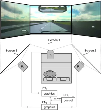
1. First, the virtual scene was optimized aiming at a reduction in optical flow (Fig. 1). Optical flow depends on the virtual environment and objects such as build-ing and trees close to the road generate more optical flow. therefore, objects along roads (i.e., houses, street lamps) were removed and road side and surface were homogenized.
2. as a second modification, an IVB was implemented. the IVB is a component in the virtual scene that pro-vides visual motion and orientation cues that match those from the vestibular receptors [14]. In our study, a static, thin (3 mm, 4 cycles per radian), black grid IVB was superimposed over the entire virtual scene (Fig. 2). 3. third, brightness of the lateral projection screens was
decreased by 48 % (Fig. 2) to further reduce optical flow. thereby, the contrast of the lateral projection screens became decreased which leads to a decrease of optical flow [21].
2.4 apparatus
2.4.1 Driving simulator
a fixed-based driving simulator (F12PI-3/a88, Foerst gmbH) setup was used to create the simulation environ-ment. three projectors (Ultra Short Focus lCD projector, Sanyo) with 1,024 × 768 pixel resolution project the image onto three canvases (1.80 × 1.39 m). the canvases form a 120° angle and are positioned in front of the participant, creating a 180° horizontal and 40° vertical field of view. three computers with Microsoft Windows 7 operating sys-tem (Microsoft Corp.) are used to control the simulation. One computer calculates and controls the dynamic sce-nario, and the other two computers render the graphics at 35 Hz. to avoid interferences as well as distractions to the driver, the driving simulator is installed in a temperature-, light-, and noise-controlled room (Fig. 3).
2.4.2 Sensory systems
While the participant was immersed to the virtual world, eye movements, heart rate, respiratory rate, skin tempera-ture, and skin conductance were measured. Eye movements were recorded by using a head-free eye-tracker with video-based/corneal reflection tracking (SMI iView X HED, 50 Hz). two cameras were used—one to capture the pupil and the corneal reflection and one to film the scene. the outcome variables of the eye-tracking measurements were
Fig. 1 Upper images show screenshots of the high-SCS (left) and
low-SCS as participants are seeing them recoded with the scene camera from the head-mounted eye-tracker. In the lower images, the
optical flow during 0.04 s (25 frames per second) of the two scenes is shown in gray scale. Optical flow was calculated using Horn and Schunck’s algorithm [21]
Fig. 2 Screenshots of high-SCS (upper image) and low-SCS scene. low-SCS scene was optimized with respect to reduce optical flow and
fixation durations and saccade amplitudes, which were stored on a separate computer.
Heart rate was measured using a photoelectric pulse sensor for pulsatile blood flow (g.PUlSEsensor, g.tec medical engineering gmbH). the sensor was positioned at the volar surface of the distal phalanx of the index fin-ger. Skin conductance was recorded with a galvanic skin response sensor (g.gSrsensor, g.tec medical engineer-ing gmbH) at the volar surfaces of the distal phalanxes of the third and fourth fingers of the left hand. a thermistor flow sensor (g.SlEEPsensor, g.tec medical engineering gmbH) was used to get respiratory rate (nose and mouth). Skin temperature was measured using a thermistor YSI 400 (g.tEMPsensor, g.tec medical engineering gmbH), which was attached at the volar surface of the distal phalanx of the fifth finger. Heart rate, respiratory rate, skin temperature as well as skin conductance were amplified with a Datalink amplifier (Biometrics ltd.) and sampled with 1,000 Hz. Signals were not filtered before data analysis.
2.5 Data analysis
all data were calculated as mean values for time frames of 60 s for the experimental period of 10 min as well as 5 min before and 1 min after immersion. Matlab r2011a (the MathWorks, Inc.) was used to conduct the data analysis.
Mean duration of saccades and fixations as well as sac-cade amplitudes were calculated directly from the eye-tracking system using the corresponding event marker (SMI). Minimal fixation duration was defined as 80 ms. to quantify heart rate and respiratory rate, a low-pass fil-ter was applied and a peak detection algorithm was used to count peaks per minute. Signal amplitudes were not taken into account. Skin conductance and temperature were con-tinuous signals where mean values of every minute (ampli-tude) were calculated. nonparametric Wilcoxon rank-sum test was used to test significance of the differences between the measures in the high-SCS and the low-SCS. Further-more, linear regression was calculated to show depend-ency of the change in SSQ score and the change in saccade amplitudes.
3 Results
3.1 Simulator Sickness Questionnaire
all participants rated the SSQ before and after both the high-SCS and low-SCS scene. Figure 4 shows the mean values of the SSQ. Before driving in the high-SCS, mean SSQ score was 105.25 (SE 27.8), while the score was 148.01 (SE 26.8) before the low-SCS scene. after 10-min driving in the high-SCS, the SSQ score increased by 122.9 % (p = 0.002) compared to an increase of 3.4 % (p = 0.878) after driving in the low-SCS. the difference of the change in SSQ between the high-SCS and the low-SCS was statistically significant with p = 0.005.
note that the results trend to differ among genders (Fig. 4, right). In the high-SCS, female subjects (N = 10) reported a mean increase of SHE by 160.98 points (p = 0.038), while males (N = 10) rated SHE 97.81 points higher (p = 0.019). this difference showed a trend with
p = 0.073. In the low-SCS, female subjects rated SHE 24.98 points higher (p = 0.620), while in the male group, a decrease of 14.91 points (p = 0.748) was measured. 3.2 Physiological measures
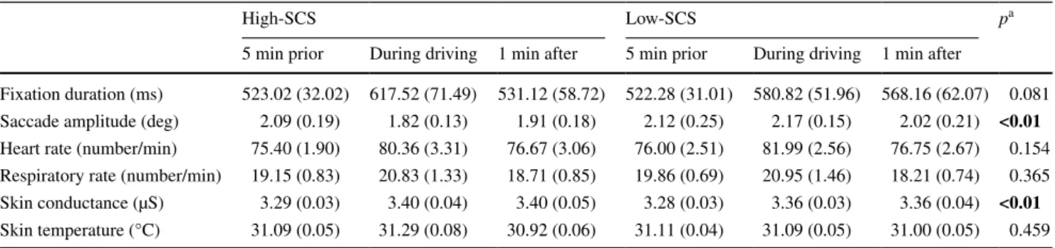
In table 1, mean values of different physiological meas-ures are summarized for both scenes. While differences in heart rate, respiratory rate, and skin temperature were less noticeable, skin conductance was significantly lower and saccade amplitudes were higher in the low-SCS.
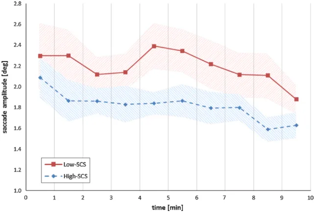
the mean saccade amplitudes during driving are in the low-SCS 16.1 % (p < 0.01) higher compared to the high-SCS (Fig. 5). also, in the low-SCS scene, the mean fixation duration is 6.3 % (p = 0.081) smaller than in the high-SCS scene. In both scenes, the difference between before and during driving is not significant (phigh = 0.320,
control graphics graphics TCP/IP PC1 PC2 Screen 2 Screen 3 P1 P2 P3 PC3 Screen 1
Fig. 3 top-down view (schematic) of the experimental setup (P1–3:
projectors). PC1 controls the dynamic scenario, while PC2 and PC3
render the graphics at 35 Hz. the participant was sitting in the driv-ing simulator’s chassis, which is based on authentic original design
plow = 0.671). Furthermore, the cumulated fixation time in the center of the image (<10° eccentricity) versus the periphery (>10° eccentricity) were calculated. In the low-SCS, the mean value and standard deviation of the time spent in the center are 58.3 ± 6.6 % versus the high-SCS 63.5 ± 8.7 % of the total cumulated fixation time. the dif-ference of 5.2 % is statistically significant with p = 0.006.
Figure 6 shows the progress of skin conductance. at the beginning, skin conductance starts increasing significantly (p < 0.001) in both scenes and reaches a plateau. Com-pared to the high-SCS, in the low-SCS skin, conductance is 13.8 % smaller (p < 0.01) during driving. no significant differences prior the experiment and during experiment were found for the other physiological measures.
3.3 Correlation SSQ: physiological measures
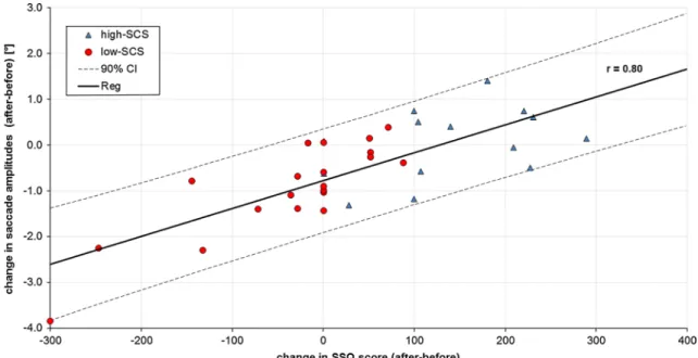
linear regression was calculated between the change of SSQ score and saccade amplitudes as well as skin conduct-ance. Strong correlation of r = 0.80 was found for saccade
amplitudes (Fig. 7) and weak correlation for skin conduct-ance (r = 0.34). Positive SSQ scores (x axis) mean that symptoms of SHE increased during driving in the simula-tor, while scores <0 mean a decrease of symptoms. Since not the difference between the two scenes are of interest, the values of both the high-SCS and the low-SCS were taken into account (N = 40).
4 Discussion
the primary aim of this study was to describe and inves-tigate a combination of three methods to evaluate whether they reduce SHE. the methods were (1) scene optimization aiming at a reduction in optical flow, (2) superimposing of an IVB, and (3) decrease of brightness of lateral projection screen to further reduce optical flow.
When comparing the SSQ score before and after driving in the simulator, in the high-SCS, the SSQ score increased by 122.9 % while in the low-SCS, only a minor increase
0 50 100 150 200 250 300 350 400 SSQ score [-] 0 50 100 150 200 250 300 350 400 SSQ score [-]
before after before after
high-SCS low-SCS
p = 0.002 p = 0.878 female (N=10)
male (N=10)
p = 0.019
before after before after
high-SCS low-SCS
p = 0.038
p = 0.620 p = 0.748
Fig. 4 Bar plots of mean values of the Simulator Sickness
Question-naire before and after both the high-SCS and low-SCS scene. Left plot represents scores of both genders (N = 20); right plot shows
results female (N = 10) and male (N = 10) separately. Error bars represent the standard error
Table 1 Summary of the mean values and standard errors (SE) of the physiological measures recorded during simulated driving in the high-SCS
and the low-SCS
Significant p-values are in bold
a p value computed between high-SCS and low-SCS during driving
High-SCS low-SCS pa
5 min prior During driving 1 min after 5 min prior During driving 1 min after
Fixation duration (ms) 523.02 (32.02) 617.52 (71.49) 531.12 (58.72) 522.28 (31.01) 580.82 (51.96) 568.16 (62.07) 0.081 Saccade amplitude (deg) 2.09 (0.19) 1.82 (0.13) 1.91 (0.18) 2.12 (0.25) 2.17 (0.15) 2.02 (0.21) <0.01 Heart rate (number/min) 75.40 (1.90) 80.36 (3.31) 76.67 (3.06) 76.00 (2.51) 81.99 (2.56) 76.75 (2.67) 0.154 respiratory rate (number/min) 19.15 (0.83) 20.83 (1.33) 18.71 (0.85) 19.86 (0.69) 20.95 (1.46) 18.21 (0.74) 0.365 Skin conductance (µS) 3.29 (0.03) 3.40 (0.04) 3.40 (0.05) 3.28 (0.03) 3.36 (0.03) 3.36 (0.04) <0.01 Skin temperature (°C) 31.09 (0.05) 31.29 (0.08) 30.92 (0.06) 31.11 (0.04) 31.09 (0.05) 31.00 (0.05) 0.459
of 3.4 % was observed. this result supports strongly the hypothesis that the combination of the three methods sig-nificantly reduces SHE. this is true for both genders, but
the effects are more pronounced in female participants, who seems to be more susceptible to SHE and would ben-efit the most from the proposed methods to reduce SHE.
Fig. 5 Progress of saccade amplitudes during 10-min driving in the simulator. Mean values of each minute was calculated. Shaded area
repre-sents the standard error
Fig. 6 Progress of skin conductance during 10-min driving in the simulator, and 1 min before and after immersion. Mean values of each minute
the gender differences have also been noticed by others [1,
30, 38]. note that the SSQ score before driving depends on participant’s actual condition and was, therefore, not the same at the 2 days. In this study, the change in SSQ score caused by the immersion into a virtual driving scene was relevant.
Besides lower SSQ scores, all subjects also showed lower skin conduction when driving the low-SCS compared to driving the high-SCS (Fig. 7). the difference is signifi-cant and the correlation between SHE, SSQ, and skin con-duction was also observed by others, who concluded that skin conduction is an important indicator for SHE [3, 29,
36]. the differences in heart rate, respiratory rate, and skin temperature between the two scenes are less noticeable than the difference in skin conductance. also this has been observed by others, and Bertin et al. [3] concluded that skin conductance is probably the most reliable physiological SHE indicator.
In addition to these measures, we recorded fixation durations and saccade amplitudes. Saccade amplitudes showed significant differences between the high-SCS and the low-SCS, while fixation durations showed a trend. In the low-SCS, fixation duration is on average 6.3 % shorter compared to the fixations duration when driving in the high-SCS. Furthermore, the saccade amplitudes are 16.1 % higher in the low-SCS. Strong correlation between the change of saccade amplitudes and SSQ scores was found (r = 0.80). Compared to a correlation between skin conductance and SSQ, saccade amplitudes seem to be a reliable measure for SHE. no previous study has related saccade amplitudes to SSQ-assessed SHE. there
are several explanations why SHE goes together with decreased saccade amplitudes. It could be that reducing eye movements is a compensation strategy of the visual system to reduce the amount of optical flow. against this assumption speaks the saccadic omission that refers to a lack of awareness of the motion across the retina that is generated during a saccade [7, 46]. this is the result of a visual saccadic suppression, which is the selective block-ing of the visual processblock-ing durblock-ing eye movements [46]. another explanation for the reduced saccade amplitudes in the high-SCS is that under the influence of SHE, the subject tries to minimize the difference of the optical flow that is perceived via the left and the right hemifield of vision. this difference is smallest when looking at the center of the scene. that would also explain the reduced saccade amplitudes in the high-SCS. this assumption is in favor with our finding, that the cumulated fixation time spent in the center of the image (<10° eccentricity) is 5.2 % (p = 0.006) smaller in the low-SCS compared to the high-SCS.
During the 10-min drive, the participants had to react to different scenarios: For example (1) react to a deer jumping on the street, including an emergency brake or (2) driving on a narrow road because of road works. While the former example (1) causes the skin conductance to increase, the second one (2) leads to a decrease of skin conductance and let the subject calm down. Between minute two and four of the simulated drive, there are more scenarios where the par-ticipant has to react to, which leads to an increase in skin conductance and a decrease in saccade amplitudes. this explains the drop of saccade amplitudes in the first minutes
(see Fig. 5) in the low-SCS and the drop of skin conduct-ance in high-SCS after 7 min.
We asked the test subjects whether they were disturbed by the IVB, but none of them even noticed the IVB. We observed the same for the decreased luminosity of the two lateral projection screens. also, we observed that the low-SCS was much better accepted by the test persons than the high-SCS.
the reduction of scene complexity might have an influ-ence on the driving performance. therefore, we compared in post-analysis the driving performance in both scenes, and total number of errors, speed variability, lateral accel-eration, time on brake pedal, and time to collision were evaluated. none of these parameters differed significantly in both scenes.
the strength of this study is that the measurements were conducted on two different days, with at least 1 day in between, at the same time of day. also, the participants were instructed to eat the same on the 2 days. Further-more, the test population is homogenous in age, gender, computer skills, and driving experience. the combina-tion of SSQ and physiological measures is an addicombina-tional advantage.
a limitation of the study is that we applied a combina-tion of three methods, and we cannot determine how much each individual method contributes to the observed reduc-tion of SHE. In this paper, we combine three modificareduc-tions to reduce SHE during simulated driving. While others have studied single modifications (i.e., IVB [39]), no study has measured the effects of a combination of the three modi-fications. In this work, we show that the combination of the three modifications has significant effects on SHE, and these modifications can be recommended to other research-ers as well. For future studies, it would be interesting to study the effects of the individual modifications in sin-gle conditions. Prothero et al. [39] used an IVB only and reduced SSQ score by 19.8 %. When we calculate the delta of SSQ score in the low-SCS and high-SCS and compare them, we found a reduction of 96.1 % which is statistically significant with p = 0.005. With this in mind and based on our observations, we believe that the reduction of scene content has the greatest influence to reduce SHE. Further-more, the decrease of brightness is in favor to avoid flicker perception, which has been linked to SHE [30]. Due to the fact that the peripheral visual system is more sensitive to flicker than the fovea [4], the decrease of brightness in the two lateral projection screens is beneficial to avoid SHE. However, for future research, the influence of each method should be analyzed. While the influence of the IVB was already shown by others [12, 14, 34, 39], the contribution of the decrease of brightness should be further investigated (particularly with regard to the influence on optical flow and flicker). In addition, the impact on training efficiency
due to degraded virtual reality by superimposing an IVB and simplifying urban scenarios needs to be investigated. Furthermore, the medium-sized number (N = 20) could be a limiting factor of the validity of our study.
Susceptibility to SHE differs among age groups [30]. therefore, for future work, it would be interesting to con-duct a similar study in other age groups (i.e., with older participants). Moreover, the critical optical flow when sub-jects start to feel symptoms of SHE could be interesting and could contribute to optimizing our adaptations.
In summary, the results indicate that the combination of the three methods will reduce SHE in fixed-based DS, which may improve the user comfort and may reduce drop-out rates. therefore, we can recommend these methods to other researchers as well.
References
1. allen rW, Park g, Cook M, rosenthal tJ, Fiorentino D, Viirre E (2003) novice driver training results and experience with a PC based simulator. In: Proceedings of the 2nd international driving symposium on human factors in driver assessment, training and vehicle design
2. Bertin r, Collet C, Espié S, graf W (2005) Objective measure-ment of simulator sickness and the role of visual-vestibular con-flict situations. In: Driving simulation conference north america 3. Bertin r, guillot a, Collet C, Vienne F, Espié S, graf W (2004)
Objective measurement of simulator sickness and the role of visual-vestibular conflict situations: a study with vestibular-loss (a-reflexive) subjects. In: Proceedings of neuroscience meeting, San Diego
4. Boff Kr, lincoln JE (1988) Engineering data compendium: human perception and performance, vol 3. armstrong aerospace Medical research laboratory, Ohio
5. Brooks JO, goodenough rr, Crisler MC, Klein nD, alley rl, Koon Bl, logan WC Jr, Ogle JH, tyrrell ra, Wills rF (2010) Simulator sickness during driving simulation studies. accid anal Prev 42(3):788–796
6. Brown lB, Ott Br (2004) Driving and dementia: a review of the literature. J geriatr Psychiatry neurol 17(4):232–240
7. Campbell FW, Wurtz rH (1978) Saccadic omission: why we do not see a grey-out during a saccadic eye movement. Vis res 18(10):1297–1303
8. Classen S, Bewernitz M, Shechtman O (2011) Driving simulator sickness: an evidence-based review of the literature. am J Occup ther 65(2):179–188
9. Cobb SVg, nichols S, ramsey a, Wilson Jr (1999) Virtual real-ity-induced symptoms and effects (VrISE). Presence teleoper Virtual Environ 8(2):169–186
10. Cowings PS, Suter S, toscano WB, Kamiya J, naifeh K (1986) general autonomic components of motion sickness. Psychophys-iology 23(5):542–551
11. Yong gI (2012) Effects of age and gender differences on automo-bile instrument cluster design. advances in affective and pleasur-able design. CrC Press, Boca raton, Fl, pp 22–212
12. Duh HB-l, Parker DE, Furness ta (2001) an independent visual background reduced balance disturbance envoked by visual scene motion: implication for alleviating simulator sickness. In: Pro-ceedings of the SIgCHI conference on human factors in comput-ing systems, Seattle, Washcomput-ington, USa. aCM, pp 85–89
13. Duh HBl, abi-rached H, Parker DE, Furness ta (2001) Effects on balance disturbance of manipulating depth of an independent visual background in a stereographic display. In: Proceedings of the human factors and ergonomics society annual meeting 14. Duh HBl, Parker DE, Furness ta (2004) an independent visual
background reduced simulator sickness in a driving simulator. Presence teleoper Virtual Environ 13(5):578–588
15. Fisher D, Pollatsek a, Pradhan a (2006) Can novice drivers be trained to scan for information that will reduce their likelihood of a crash? Inj Prev 12(Suppl 1):i25–i29
16. Fisher Dl (2011) Handbook of driving simulation for engineer-ing, medicine, and psychology. CrC Press, Boca raton
17. gianaros PJ, Muth Er, Mordkoff Jt, levine ME, Stern rM (2001) a questionnaire for the assessment of the multiple dimen-sions of motion sickness. aviat Space Environ Med 72(2):115 18. gibson JJ (1986) the ecological approach to visual perception.
routledge, london
19. Hettinger lJ, Berbaum KS, Kennedy rS, Dunlap WP, nolan MD (1990) Vection and simulator sickness. Mil Psychol 2(3):171–181 20. Hill K, Howarth P (2000) Habituation to the side effects of
immersion in a virtual environment. Displays 21(1):25–30 21. Horn BKP, Schunck Bg (1981) Determining optical flow. artif
Intell 17(1):185–203
22. Howarth P, Costello P (1997) the occurrence of virtual simula-tion sickness symptoms when an HMD was used as a personal viewing system. Displays 18(2):107–116
23. Hu S, grant WF, Stern rM, Koch Kl (1991) Motion sickness severity and physiological correlates during repeated expo-sures to a rotating optokinetic drum. aviat Space Environ Med 62(4):308–314
24. Johnson DM (2005) Introduction to and review of simulator sick-ness research. US army research Institute for the Behavior Sci-ences, arlington
25. Kartiko I, Kavakli M, Ken C (2009) the impacts of animated-virtual actors’ visual complexity and simulator sickness in animated-virtual reality applications. In: Sixth international conference on com-puter graphics, imaging and visualization
26. Kellogg rS, Kennedy rS, graybiel a (1964) Motion sickness symptomatology of labyrinthine defective and normal subjects during zero gravity maneuvers. aerosp Med 36:315–318
27. Kennedy rS, lane nE, Berbaum KS, lilienthal Mg (1993) Sim-ulator sickness questionnaire: an enhanced method for quantify-ing simulator sickness. Int J aviat Psychol 3(3):203–220
28. Kennedy rS, lane nE, grizzard MC, Stanney KM, Kingdon K, lanham S (2001) Use of a motion history questionnaire to pre-dict simulator sickness. In: Driving simulation conference 29. Kim YY, Kim HJ, Kim En, Ko HD, Kim Ht (2005)
Character-istic changes in the physiological components of cybersickness. Psychophysiology 42(5):616–625
30. Kolasinski EM (1995) Simulator sickness in virtual environ-ments. technical report of the U.S. army research Institute 1027 31. lee HC, Cameron D, lee aH (2003) assessing the driving per-formance of older adult drivers: on-road versus simulated driving. accid anal Prev 35(5):797–803
32. lee HC, lee aH, Cameron D, li-tsang C (2003) Using a driving simulator to identify older drivers at inflated risk of motor vehicle crashes. J Saf res 34(4):453–459
33. lerman Y, Sadovsky g, goldberg E, Kedem r, Peritz E, Pines a (1993) Correlates of military tank simulator sickness. aviat Space Environ Med 64(7):619–622
34. lin JJW, abi-rached H, Kim DH, Parker DE, Furness ta (2002) a “natural” independent visual background reduced simulator sickness. In: Proceedings of the human factors and ergonomics society annual meeting
35. lukas a, nikolaus t (2009) Driving ability and dementia. Zeitschrift fur gerontologie und geriatrie: Organ der Deutschen gesellschaft fur gerontologie und geriatrie 42(3):205
36. Min BC, Chung SC, Min YK, Sakamoto K (2004) Psychophysi-ological evaluation of simulator sickness evoked by a graphic simulator. appl Ergon 35(6):549–556
37. Mourant rr, rengarajan P, Cox D, lin Y, Jaeger BK (2007) the effect of driving environments on simulator sickness. In: Pro-ceedings of the human factors and ergonomics society annual meeting
38. Mourant rr, thattacherry tr (2000) Simulator sickness in a virtual environments driving simulator. In: Proceedings of the human factors and ergonomics society annual meeting
39. Prothero JD, Draper MH, Furness ta, Parker DE, Wells MJ (1999) the use of an independent visual background to reduce simulator side-effects. aviat Space Environ Med 70(3):277–283 40. Prothero JD, Draper MH, Furness ta, Parker DE, Wells MJ
(1997) Do visual background manipulations reduce simula-tor sickness. In: Proceedings of the international workshop on motion sickness: medical and human factors
41. reason Jt, Brand JJ (1975) Motion sickness. academic Press, Oxford, 310 pp
42. regan C (1995) an investigation into nausea and other side-effects of head-coupled immersive virtual reality. Virtual real 1(1):17–31
43. Schultheis Mt, rizzo aa (2001) the application of virtual real-ity technology in rehabilitation. rehabil Psychol 46(3):296 44. Stanney KM, Mourant rr, Kennedy rS (1998) Human factors
issues in virtual environments: a review of the literature. Presence 7(4):327–351
45. Ungs tJ (1989) Simulator induced syndrome: evidence for long-term after effects. aviat Space Environ Med 60:252–255
46. Watson tl, Krekelberg B (2009) the relationship between saccadic suppression and perceptual stability. Curr Biol 19(12):1040–1043
47. Yin Z, Mourant rr (2009). the perception of optical flow in driving simulators. In: Proceedings of the 5th international driv-ing symposium on human factors in driver assessment, traindriv-ing, and vehicle design