Special Issue
Ulrich Schwesinger*, Pietro Versari, Alberto Broggi, and Roland Siegwart
Vision-only fully automated driving in dynamic
mixed-traffic scenarios
DOI 10.1515/itit-2015-0005
Received March 15, 2015; revised June 12, 2015; accepted June 23, 2015
Abstract: In this work an overview of the local
mo-tion planning and dynamic percepmo-tion framework within the V-Charge project is presented. This framework en-ables the V-Charge car to autonomously navigate in dy-namic mixed-traffic scenarios. Other traffic participants are detected, classified and tracked from a combination of stereo and wide-angle monocular cameras. Predictions of their future movements are generated utilizing infras-tructure information. Safe motion plans are acquired with a system-compliant sampling-based local motion planner. We show the navigation performance of this vision-only autonomous vehicle in both simulation and real-world ex-periments.
Keywords: Automotive, autonomous navigation, motion
planning, environment perception.
ACM CCS: Computing methodologies → Artificial intel-ligence → Control methods → Motion path planning, Computing methodologies → Artificial intelligence → Computer vision→Computer vision tasks→Vision for robotics
1 Introduction
Autonomous navigation in mixed-traffic scenarios re-quires a broad spectrum of robotic disciplines like localiza-tion, perceplocaliza-tion, classificalocaliza-tion, motion planning and con-trol to perform at their peak. The vehicle needs to precisely perceive its local surrounding and compute safe motion
*Corresponding author: Ulrich Schwesinger, Autonomous Systems
Lab, Institute of Robotics and Intelligent Systems, ETH Zurich, e-mail: [email protected]
Pietro Versari, Alberto Broggi: VisLab, Department of Information
Engineering, University of Parma
Roland Siegwart: Autonomous Systems Lab, Institute of Robotics
and Intelligent Systems, ETH Zurich
plans at a high rate in order to react quickly to unfore-seen events. Those components experienced significant advances within the last decade – especially since the im-petus of the DARPA Urban Challenge in 2007 [1–4]. Since then, effort from various groups was spent to bring au-tonomous driving capabilities to public streets. With their BRAiVE platform [5], the Artificial Vision and Intelligent Systems Laboratory (VisLab) successfully demonstrated autonomous navigation in rural roads, highways and ur-ban environments during the PROUD run [6]. BRAiVE’s sensor setup consisted of in total ten cameras, five laser scanners and a GPS+IMU solution. Carnegie Mellon’s Cadillac SRX completed a53km long route on public roads without human intervention [7]. Similar to VisLab’s au-tonomous vehicle, Carnegie Mellon’s self driving car uti-lized a mixture of laser scanners, lidars and cameras. Daimler’s “Intelligent Drive” system autonomously drove 103km on rural roads, small villages and major cities us-ing a combination of vision- and radar sensors [8] and Google’s self driving cars spent remarkable1 126 500km on public US streets in autonomous mode up to now [9].
For environment perception, all the above mentioned platforms complemented vision sensors with other po-tentially costly sensors such as laser scanners, lidars or
radars. Within the European project V-Charge (Automated Valet Parking and Charging for e-Mobility) the applica-tion of low-speed autonomous driving in restricted park-ing areas with low-cost vision sensors only is targeted. Low-cost sensors already available in series cars will lower the consumer price for the additional autonomous navi-gation functionality and in the end lead to a higher cus-tomer acceptance of those systems. As legal issues might prevent the acceptance of autonomous vehicles in pub-lic traffic for a foreseeable time, the project aims at the application of autonomous functionality in restricted ar-eas such as parking lots. Here, automated vehicles consti-tute a convenient solution for approaching vacant parking spots and charging stations (electric vehicles) and provide a valuable drop-off/pick-up service at the entrance of the parking lot.
The V-Charge vehicle features static obstacle avoid-ance as well as the handling of mixed-traffic scenarios where automated and human-operated cars share a com-mon workspace and have to interact with each other. Nav-igation has to be accomplished in tight spaces with pedes-trians and other vehicles in close proximity to the ego ve-hicle. These tasks are accomplished with a sensor suite solely comprised of two stereo cameras, four monocular wide angle fisheye cameras, twelve stock ultrasonic sen-sors and incremental encoders at the vehicle’s wheels.
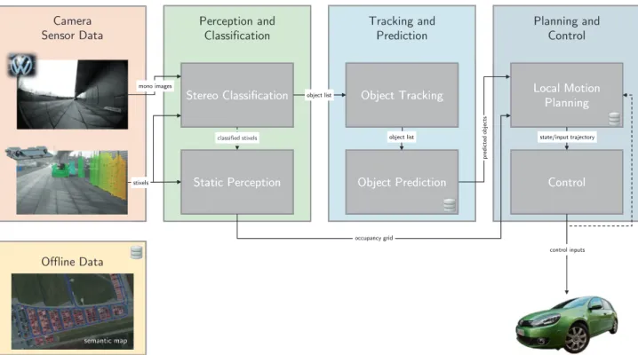
Figure 2: Overview of software modules involved in on-lane navigation. The processing chain reaches from raw sensor data (left) to the
system inputs sent to the platform (right).
2 System overview
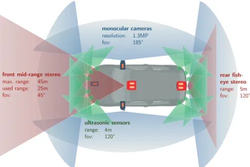
A high-level overview of the V-Charge system is depicted in Figure2. From left to right the processing chain is visual-ized starting with the sensor data and eventually resulting in system inputs to the vehicle. The key sensors to perceive the environment are the front stereo camera as well as the front and side monocular cameras. Specifications and cov-erage information are illustrated in Figure3. The rear fish-eye stereo sensor as well as the ultrasonic sensors are used for close-range obstacle detection during parking maneu-vers. The ultrasonic sensors additionally serve as the in-put to an emergency brake module. The 2.5D stixel outin-put of the front stereo sensor is on the one hand used to cre-ate a two-dimensional (2D) occupancy grid of the environ-ment, containing static information only. Stixels assigned to dynamic objects are removed from the grid. On the other hand, together with the images from the front monocular camera, it forms the input of the “Stereo Classification” module, which groups stixels to objects and assigns class labels to them from a database of known object classes. This module is described in detail in Section3. The clas-sified objects are tracked with an extended Kalman filter, applying suitable motion models for propagation based on the classification result. Once classified and tracked, predictions of the future movement of objects are
gener-range
Figure 3: Schematic sensor coverage
of the V-Charge setup suite.
ated, taking into account the object’s dynamic model and further infrastructure information such as the road net-work stored in a semantic map database. The “Local Mo-tion Planning” module described in SecMo-tion4computes a safe motion plan based on the latest perceptual informa-tion and forwards the plan in form of a time-stamped se-quence of reference states plus feed-forward system inputs to an underlying “Control” module. The “Control” mod-ule takes care of correcting modeling errors from the “Lo-cal Motion Planning” module. The system inputs from the control module are fed back to the local motion planner to correctly propagate the system states during the expected cycle time of the planner and to model system dead times.
3 Stereo object classification
To better understand the surrounding environment and predict its evolution over time, it is important to distin-guish between static obstacles and dynamic objects, as well as between different object types. Our approach is similar to the one presented in [10]. A classifier is used to detect pedestrians and vehicles, and stereo stixel informa-tion is used to increase both accuracy and computainforma-tional speed. In contrast to [10], we utilize stixel information from the stereo sensor to obtain object hypotheses via an initial clustering step. A class label from a database of dynamic objects is then assigned to each object hypothesis using a classifier operating on monocular fisheye images trained on publicly available datasets. Though the current object database only contains pedestrians and vehicles, adding more classes is a straightforward process.
3.1 Unwarping of fisheye images
As the front stereo system has a limited field of view, nearby objects are potentially only partially visible with the stereo sensor, whereas they still appear in the field of view of the front fisheye camera. This can happen for in-stance if a pedestrian is walking close to the front of the ve-hicle. The stereo system will still detect the pedestrian, but its upper part is outside the stereo system’s field of view. By projecting stixels from stereo hypothesis in the wide-angle images obtained by the front fisheye camera, the stereo ob-ject classification is able to utilize the full information of the wide-angle monocular view.
Fisheye lenses provide very large wide-angle views – theoretically the entire front hemispheric view of180∘– but the images suffer from severe distortion since the hemi-spherical scene gets projected onto a flat surface. To cor-rect the fisheye lens distortion, the image is reprojected onto a virtual plane in order to obtain a pinhole image, as shown in Figure4.
3.2 Classification
Each object class stores suitable ranges for the object’s size and aspect ratio. Those restrictions are used in a pre-filter step to eliminate hypothesis not coherent with the specific class characteristics. Each object passing the pre-filter step is projected onto the pinhole image and, for each candi-date object class, a region of interest (ROI) is computed. This process takes into account several factors: the object’s distance and its dimension in the image domain, the class
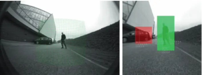
Figure 4: Example of a front fisheye camera image (on the left) and
the related un-warped image used in the “Stereo Object
Classification” stage (on the right). The left figure depicts the virtual plane used to obtain the pinhole image. For classification, object hypothesis are projected onto the pinhole image in order to define a ROI for the classifier. The ROI for the vehicle class is depicted in red, whereas the ROI for the pedestrian class is marked in green.
aspect ratio and the extrinsic calibration of the camera. An example of the output of this step is shown in the right part of Figure4.
Every ROI is classified by a Soft-Cascade+ICF fier to assign a label to the related hypothesis. The classi-fier is based on the improved version of the Integral Chan-nel Feature (ICF), where a soft-cascade technique is used to speed up the algorithm and reduce CPU load [10]. The classifier differs from [10] since no LUV color channels are available. ICF are more discriminative than e. g. Haar fea-tures [11], providing a faster rejection of false positives and resulting in a higher detection rate and faster computation times. In our approach, a shared pre-processing phase be-tween pedestrian and vehicle detection is used to further speedup the detector.
One classifier with a dimension of38×38pixels is used for vehicles, whereas a32 × 64pixels and a48 × 96pixels classifier are used for pedestrians. For each classifier four scales are computed in total. We decided to use two clas-sifiers with different dimensions for pedestrians in order to be able to classify small objects and to be accurate in close proximity to the car at the same time. Figures14and
13visualize the result of this module during online naviga-tion, where each classified object is marked with a colored bounding box according to the assigned object class (red: vehicle, green: pedestrian). Classify only these ROI signifi-cantly reduces both false positives and computation time, as it is shown in [10].
4 System-compliant motion
planning among other traffic
participants
The information from static environment perception, ob-ject prediction and a high-level plan from a topological planner operating on the roadgraph data structure are pro-cessed in a fast on-lane local motion planner, first pre-sented in [12]. The local motion planner handles both static and dynamic mixed-traffic scenarios such as pedestrian avoidance, oncoming traffic and platooning.
4.1 On-lane motion planning
The local motion planner operates in a sampling-based manner, generating numerous system-compliant candi-date motions along a reference path in a tree-like fash-ion. This trajectory roll-out scheme is widely used for automotive applications [2,13,14], however differs from these related works in the way candidate motion tives are constructed. Instead of using geometric primi-tives or parametrized functions that might not conform with the non-holonomic system model of a car and have to be pruned from the candidate motion set at a later stage, the candidate motions in this approach are constructed via a forward simulation of a detailed Ackermann vehicle model. In conjunction with a simulated controller, regulat-ing the system towards samples of a manifold aligned with the reference path, these candidate motions are drivable by construction and the approach is able to model chal-lenging system characteristics such as dead times and ac-tuator limits easily. The computation time of the forward simulation is compared to the computational burden of collision detection still low.
During tree generation, samples𝑚 = (𝑑ref, 𝑣ref, 𝑘𝑣,ref) are iteratively drawn from a set𝑀of a discretized state manifold and used as target states for closed-loop sys-tem control, where(𝑑ref, 𝑣ref, 𝑘𝑣,ref)stand for a desired lat-eral offset, a desired speed and a proportional gain for a simulated velocity controller respectively. The state man-ifold consists of all states that are heading- and curvature-aligned with the global reference path. A candidate mo-tion is then constructed using a user-supplied vehicle controller𝑔, that generates a sequence of system inputs
𝑢(𝑡) = 𝑔(𝑥(𝑡), 𝑚)to regulate the forward-simulated sys-tem model𝑓, with
Figure 5: Navigation in the presence of localization errors in lateral
direction (top, 1 m) and orientation (bottom, 7°).
towards the sample 𝑚 over a fixed time period, 𝑇sim. Through the forward simulation of the vehicle model, the approach is able to handle discontinuities in the reference path. If localization errors occur in lateral direction, local obstacle information is usually sufficient to keep the vehi-cle operable as lateral adaptations are inherently encoded in the candidate motion set, provided that lane width in-formation does not prevent the vehicle from performing the required lateral adjustment. Localization errors in ori-entation have more severe effects as depicted in Figure5. However, localization errors in the V-Charge system are small (lateral< 2cm, orientation< 1.5°) thanks to the ma-ture visual localization framework [15,16].
The computational complexity of the approach in-creases exponentially with the depth of the tree. In the V-Charge project a tree with depth one is used, which proved to be sufficient for good navigation performance. An exem-plary candidate motion set is depicted in Figure9.
4.2 Collision detection with static and
dynamic scene elements
Fast collision detection is the bottleneck for many motion planning algorithms.
In order to test candidate motions for collision with static objects a 2D occupancy grid is used. The rectangu-lar shape of the ego vehicle is approximated by a collec-tion of𝑁disc shapes [17]. The quality of the approxima-tion of the rectangular shape improves with the number of discs used. This allows for fast collision tests of ego poses via𝑁comparisons on a distance transform of the
gridmap. Candidate motions in collision with a static ob-stacle at any point within the planning horizon are pruned. For collision-free trajectories, a soft cost term based on the minimum distance of the candidate motion to any static obstacle over time is computed. In our implementation the cost term decreases linearly up to a specified threshold dis-tance.
The collision detection technique based on a 2D map inflation is applicable only for static objects where the time parameter is negligible. However moving objects may oc-cupy the same space at a different point in time. While the majority of previously presented planning frameworks operating in dynamic environments use a naive multiple interference test for collision detection with moving jects where every robot pose is tested against every stacle and single disk approximations are used for all ob-jects, we found this method to be inappropriate for navi-gation in fairly densely occupied spaces. The disc approxi-mation is often too coarse and causes an unacceptable loss of space for navigation. Furthermore multiple interference tests with exact collision shapes (e. g. oriented boxes for vehicles) are already too slow for online operation with a fairly small amount of dynamic objects in the scene. In [18] we presented a fast and exact collision detection technique for moving objects based on a bounding volume hierarchy (BVH) data structure in workspace-time space. In our approach we utilize an axis-aligned bounding box tree to efficiently prune the majority of oriented bound-ing box collision tests. This technique allows us to run the sampling-based motion planner at a frequency of5Hz. An exemplary tree is depicted in Figure6.
In contrast to static obstacles, candidate motions in collision with dynamic objects are not pruned from the set.
t x y
Figure 6: Axis aligned bounding box tree in workspace-time space
for fast dynamic collision detection. Three obstacle trajectories are generated by a random walk (blue shades). The ego trajectory (green/red) can be efficiently tested for collision with the tree structure (wireframes).
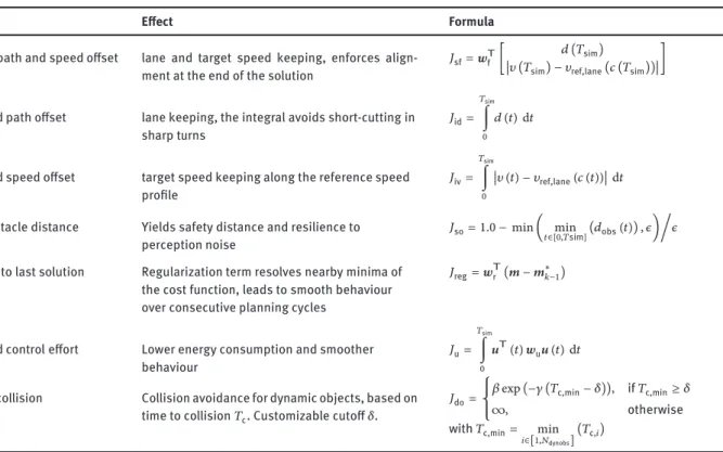
Table 1: Cost terms used in the local planning framework.
Cost term Effect Formula
Terminal path and speed offset lane and target speed keeping, enforces align-ment at the end of the solution
𝐽sf= 𝑤Tf [
𝑑 (𝑇sim)
𝑣 (𝑇sim) − 𝑣ref,lane(𝑐 (𝑇sim))
]
Integrated path offset lane keeping, the integral avoids short-cutting in sharp turns 𝐽id= 𝑇sim ∫ 0 𝑑 (𝑡) d𝑡
Integrated speed offset target speed keeping along the reference speed profile 𝐽iv= 𝑇sim ∫ 0 𝑣 (𝑡) − 𝑣ref,lane(𝑐 (𝑡)) d𝑡
Static obstacle distance Yields safety distance and resilience to perception noise
𝐽so= 1.0 − min ( min𝑡∈[0,𝑇sim](𝑑obs(𝑡)) , 𝜖)/𝜖
Deviation to last solution Regularization term resolves nearby minima of the cost function, leads to smooth behaviour over consecutive planning cycles
𝐽reg= 𝑤Tr (𝑚 − 𝑚∗𝑘−1)
Integrated control effort Lower energy consumption and smoother behaviour 𝐽u= 𝑇sim ∫ 0 𝑢T(𝑡) 𝑤u𝑢 (𝑡) d𝑡
Dynamic collision Collision avoidance for dynamic objects, based on time to collision 𝑇c. Customizable cutoff 𝛿.
𝐽do=
{ { {
𝛽 exp (−𝛾 (𝑇c,min− 𝛿)), if 𝑇c,min≥ 𝛿
∞, otherwise
with 𝑇c,min= min 𝑖∈[1,𝑁dynobs]
(𝑇c,𝑖)
Instead, an additional “soft” cost term based on the es-timated time to collision is introduced. This accounts for the fact that motion predictions of other traffic participants are inherently subject to uncertainty. Predictions become more uncertain the farther they are in the future. Therefore a cost term with exponential decay over time,𝐽do, is used (see Table1).
4.3 Objective function design
For each candidate motion a scalar cost value is computed which is comprised of different terms. In the V-Charge project significant effort was spent to design an objective function that performs well in both static and dynamic en-vironments. Each candidate motion is scored with respect to its alignment with the reference path and the lane’s ref-erence speed. Furthermore cost terms are introduced for soft penalization of close distances to static obstacles, in-tegrated steering speed and collisions with dynamic ob-jects. The cost terms and their motivations are summarized in Table1, where𝑤f,𝑤rand𝑤uare user-supplied weight vectors,𝑐(𝑡)denotes the curvilinear abscissa along the ref-erence path associated with the vehicle pose at time𝑡and
𝑚∗
𝑘−1is the optimal sample in the previous planning cycle. For a more intuitive tuning of the weights, the individual
cost terms are normalized to lie within the range[0, 1](this requires the cost of all candidate motions’ cost terms to be available). The final cost of a candidate motion for sample
𝑚nis computed via a weighted sum of the cost terms via
𝐽 (𝑚n) = 𝑤𝐽T [ [ [ [ [ [ [ [ [ [ [ norm(𝐽sf(𝑚n)) norm(𝐽id(𝑚n)) norm(𝐽iv(𝑚n)) norm(𝐽so(𝑚n) − 𝐽so,d∗ )
norm(𝐽reg,𝑛) norm(𝐽u,𝑛) 𝐺𝑑(𝐽do,𝑛) ] ] ] ] ] ] ] ] ] ] ] . (2)
In the following we will discuss certain aspects of a subset of these cost terms in more detail.
Static obstacle distance cost term
In Equation (2),𝐽so,d∗ = {𝐽so(𝑚n) | 𝑚 ∈ 𝑀, 𝑚d = 𝑚n,d}is the minimal static obstacle cost of all samples with the same lateral offset𝑑refas sample𝑚n. This yields a static obstacle cost term of zero for the sample with the largest minimum distance to any obstacle. Without this modifi-cation, narrow passages appear as high cost regions. De-pending on the ratio between the static obstacle weight and the weights influencing the longitudinal speed terms, the cost function might score candidate motions coming to
Figure 7: Influence of static obstacle distance cost term. The red
track depicts the navigation behaviour without the cost term. Obstacles are passed without safety distance. The blue track shows navigation with active static obstacle distance penalization, resulting in a safe and comfortable avoidance of the object.
Figure 8: Influence of the post-processing step 𝐽so(𝑚n) − 𝐽so,d∗
applied to the static obstacle cost term to improve navigation performance in narrow passages. Without the modification, the vehicle denies to pass the narrow passage (red track).
a full standstill in front of the narrow passage better than motions passing the high cost region induced by the static obstacle cost term. The modification encodes the intention to keep a safety distance to static obstacles if possible, but does not penalize close distances if the navigation space gets tight. This behaviour is depicted in Figures7and8.
Dynamic collision cost term
The dynamic collision detection framework returns binary answers to collision queries between candidate motions and predicted trajectories of other traffic participants. This results in an ego motion passing objects with the minimal realizable distance, rendering the planning stage vulnera-ble to measurement noise and resulting in maneuvers be-ing perceived as risky. While the BVH-based collision de-tection framework provides the possibility for accelerated distance queries between objects’ trajectories, this comes with a significant computational overhead compared to
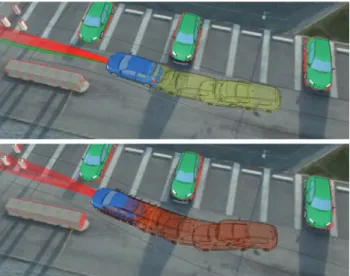
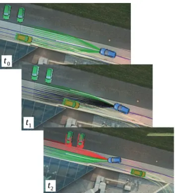
bi-nary collision tests. Inspired by [19], we instead use a Gaus-sian smoothing filter𝐺𝑑over the dynamic object cost term in the lateral offset dimension𝑑. The filter blends costs from collisions into neighboring candidate motions, yield-ing the desired side clearance without the necessity to per-form expensive distance queries. The dynamic object cost term is excluded from the normalization procedure due to its safety-critical nature. The resulting navigation be-haviour is illustrated in Figure9in a simulated run. In the beginning (upper figure), the candidate motions to the left of the blue ego vehicle already collide, however the impor-tance of the collision is low due to the exponential cost de-cay. The closer the oncoming car approaches (middle fig-ure), the higher the cost of the colliding candidate motions becomes and the ego vehicle initiates the avoidance ma-neuver. After passing the oncoming vehicle (lower figure), the ego vehicle maneuvers around two static vehicles that entered the field of view of the front stereo camera.
Reference speed
The lane’s reference speed𝑣ref,lane(𝑐)at a given curvilin-ear abscissa𝑐is read from an attribute of the road network description in the semantic map database. Lane width in-formation from the database is used to adapt the lateral offset range of the samples𝑚on-the-fly.
Figure 9: Simulated avoidance maneuver with an oncoming vehicle.
Color scheme for candidate motions: green = low cost, black = high cost, red = in collision with static obstacle.
4.4 Situation-specific adaptations
The local motion planner operates almost completely without inputs from higher-level situational awareness modules. The primary goal is to encode suitable be-haviours in the objective function of the local motion plan-ner and only to fall back on higher-level behaviour mod-ifications if necessary. For smooth platooning behaviour, the reference speed𝑣ref,laneis modified to yield a specified time-gap and/or distance between the ego vehicle and the car in front. This solely shifts the minimum of the objective function, leaving the rest of the planning framework un-changed. To determine the relevant object in front, a scor-ing metric in the lane’s Frenet-Serret frame is used based on the objects’ longitudinal and lateral distances to the ego vehicle along the lane.
5 Movement predictions for traffic
participants
Reasoning about future movements of other traffic partic-ipants is important for well-behaved navigation in mixed-traffic scenarios. Our motion prediction scheme is based on a forward simulation of different agent motion mod-els. A suitable motion model is chosen online based on the associated object class label determined by the classi-fication module. Our classiclassi-fication module and hence the motion prediction module distinguishes between pedes-trians and vehicles. As pedespedes-trians often move in uncon-ventional ways and do not respect their dedicated walk-ways rigorously (especially in parking lots the V-Charge project is dedicated to), a constant velocity model is ap-plied for pedestrians. This model is clearly limited in its predictive capabilities. In our real-world experiments out-lined in Section6the lack of interaction-awareness, taking into account the reaction of pedestrians to the ego vehi-cle, was noticeable. Well-established approaches like the Reciprocal Velocity Obstacles [20], or more recent ones such as Interacting Gaussian Processes [21] and Maximum Entropy Models [22] are promising, yet the adaptation to the semantic-rich automated driving domain and the chal-lenging system dynamics involved was not yet tackled.
In contrast to pedestrians, movements of vehicles are bound much tighter to the infrastructure. Therefore we exploit the lane information of the roadgraph to improve upon the motion predictions of vehicles. Our approach re-sembles the one presented in [23], extending it to account for common vehicle kinodynamics. In a first step, a kd-tree containing all three-dimensional (3D) poses (2D position
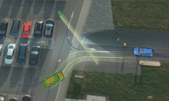
Figure 10: Movement predictions for two different agent types over
a time horizon of 10 seconds. Green boxes represent the detected bounding boxes of the objects. Yellow wireframe objects depict the predictions.
𝑥,𝑦and yaw angle𝜃) of the roadgraph is built. This allows for fast nearest neighbor queries for any vehicle pose in the 2D workspace in order to find the closest pose on the road-graph. The heading dimension is included in order to dis-tinguish between nearby lanes with opposite directions. We use a custom distance metric between two poses𝑐0and
𝑐1in𝑆𝐸(2) 𝑑2(𝑐 0, 𝑐1) = (𝑐0𝑥− 𝑐1𝑥)2+ (𝑐0𝑦− 𝑐1𝑦) 2 + 𝛼(𝑐0𝜃− 𝑐1𝜃)2 (3)
with𝛼being a scaling factor for the angular heading di-mension. During forward simulation with a discrete in-tegration scheme three operations are performed in each timestep𝑡𝑘: First, the closest pose of the simulated vehi-cle position at 𝑡𝑘 to the roadgraph is retrieved from the kd-tree. Second, the lateral offset to the closest roadgraph pose is computed and a reference pose is created by later-ally shifting the closest pose by this offset. In the third step, a control law is used to compute a desired steering angle for the simulated Ackermann model. This steering angle regulates the simulated model towards the computed ref-erence state. The speed of the vehicle is kept constant at its measured speed during the simulation time horizon. The result of this motion prediction scheme is illustrated in Fig-ure10.
6 Experimental results
In this section we provide general navigation statistics as well as real-world data for two scenarios, that frequently appear during autonomous operation on a parking lot. Within the project, the maximum speed of the vehicle is
limited to2.78m s−1while the desired speed was usually set to1.6m s−1. The local planning framework was operat-ing with a time-horizon of10s.
6.1 Motion planning statistics
Statistics were automatically generated from471GB of log files over the course of 6:47 hours of automated operation in which24.63km were covered. The results are illustrated in Figure11. In only 0.22% of the time no valid solution tra-jectory could be computed.
These events stem firstly from pedestrians moving in very close proximity to the vehicle such as the scene dis-played in Figure12. In these situations, the purely reac-tive planning approach is over-conservareac-tive. A coopera-tive prediction scheme will remedy this shortcoming and is among our current research goals. Secondly, these events sporadically occur when passing through narrow gates on the parking lot with only a few tens of centimeters margin
Figure 11: Local motion planning operation mode (left) and failure
statistics (right) generated from 24 test days over the course of two month.
Figure 12: If no valid solution trajectory could be
computed by the local motion planner, moving pedestrians in close vicinity to the ego vehicle (left) and small perception noise when passing narrow gates (right) were often the cause.
on each side of the vehicle – a highly challenging scenario for both vision-based perception and motion planning. In 0.46% of the time, the planner was keeping the car stopped in a controlled way during normal operation. While these events may occur in regular situations, they could also stem from a potential deadlock in which a global guidance would be necessary to recover the vehicle.
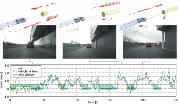
6.2 Platooning
Platooning is a situation appearing frequently in traffic. Figure13 visualizes the navigation performance during such, involving multiple stop-and-go phases. In this run, the car in front is reliably tracked throughout the complete four minutes of the run. The speed profile of the ego vehi-cle and the target car match with a slight delay induced by delays in the processing chain but mainly due to the low-pass characteristics of the drive-train. The left figure depicts the first approach to the car in front. The middle figure illustrates the local planner’s ability to concurrently adapt its plan (orange trajectory) based on static obstacle information. The static obstacle distance cost term moves the ego vehicle slightly towards the left to keep a safety dis-tance to the pillar on the right. In the rightmost figure the roadgraph-based object prediction utilizing the lane cen-ter information (blue path) is visible.
6.3 Pedestrian avoidance
Figure14depicts the navigation behaviour in the presence of a pedestrian crossing the street. The constant velocity prediction allows the vehicle to infer the future positions of the classified pedestrian agent. A lateral avoidance ma-neuver is not considered necessary, leading to a short re-duction of the ego vehicle’s speed in order to give way to
Figure 13: Real-world platooning performance in stop-and-go traffic. In this mode, the reference speed of the local motion planning
framework is adjusted based on distance and relative speed to the object in front, while obstacle avoidance is simultaneously active.
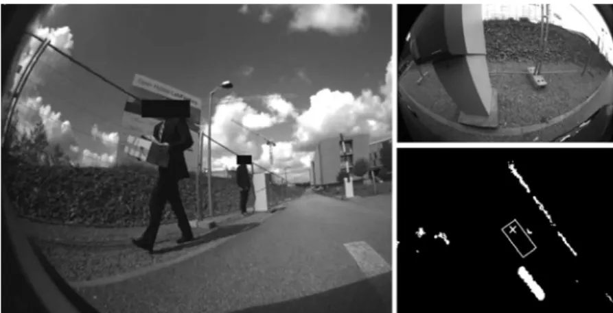
Figure 14: Real-world avoidance of crossing pedestrian. The
pedestrian is sensed by the stereo camera (red stixels) and classified as such by the stereo classification module based on the monocular camera images (top right figure). The vehicle slows down to give way to the pedestrian.
the pedestrian. Afterwards the ego vehicle speeds up again to meet its desired reference speed.
7 Conclusion
The goal of automated driving in mixed-traffic scenarios with a vision-only sensor suite is and remains
challeng-ing. The V-Charge vehicle is to our knowledge the first plat-form that does not complement the vision sensor suite with laser or lidar scanners. In this paper we reported on the on-lane planning framework and the processing chain necessary to implement smooth interaction with other traffic participants like vehicles and pedestrians. Our future research aims at extending the object detection to all available monocular cameras as well as incorporat-ing interaction-awareness in the object prediction stage by machine learning techniques to properly copy with pedes-trians in close vicinity to the vehicle.
Funding: This project has received funding from the
Eu-ropean Union’s Seventh Framework Programme for re-search, technological development and demonstration under grant agreement no 269916, V-Charge.
References
1. C. Stiller, S. Kammel, B. Pitzer, J. Ziegler, M. Werling, T. Gin-dele, and D. Jagszent, “Team AnnieWAY’s autonomous sys-tem,” Lecture Notes in Computer Science, vol. 4931 LNCS, pp. 248–259, 2008.
2. D. Ferguson, T. M. Howard, and M. Likhachev, “Motion plan-ning in urban environments,” Journal of Field Robotics, vol. 25, no. 11–12, pp. 939–960, 2008.
3. M. Montemerlo, J. Becker, S. Bhat, H. Dahlkamp, D. Dolgov, S. Ettinger, D. Haehnel, T. Hilden, G. Hoffmann, B. Huhnke,
D. Johnston, S. Klumpp, D. Langer, A. Levandowski, J. Levinson, J. Marcil, D. Orenstein, J. Paefgen, I. Penny, A. Petrovskaya, M. Pflueger, G. Stanek, D. Stavens, A. Vogt, and S. Thrun, “Junior: The stanford entry in the urban challenge,” Springer Tracts in Advanced Robotics, vol. 56, no. 9, pp. 91–123, 2009. 4. A. Broggi, A. Cappalunga, C. Caraffi, S. Cattani, S. Ghidoni,
P. Grisleri, P. P. Porta, M. Posterli, and P. Zani, “Terramax vision at the urban challenge 2007,” IEEE Transactions on Intelligent Transportation Systems, vol. 11, pp. 194–205, Mar 2010. 5. A. Broggi, M. Buzzoni, S. Debattisti, P. Grisleri, M. C. Laghi,
P. Medici, and P. Versari, “Extensive tests of autonomous driv-ing technologies,” Intelligent Transportation Systems, IEEE Transactions on, vol. 14, pp. 1403–1415, Sept 2013.
6. A. Broggi, P. Cerri, S. Debattisti, M. C. Laghi, P. Medici, M. Pan-ciroli, and A. Prioletti, “PROUD-public road urban driverless test: Architecture and results,” Proc. of the IEEE Intelligent Ve-hicles Symposium, pp. 648–654, 2014.
7. B. Spice and C. Swaney, “Carnegie mellon creates practical self-driving car using automotive-grade radars and other sen-sors,” Sept 2013. CMU Press Release, available athttp://www. cmu.edu/news/stories/archives/2013/september/sept4_ selfdrivingcar.html.
8. J. Ziegler, P. Bender, M. Schreiber, H. Lategahn, T. Strauss, C. Stiller, T. Dang, U. Franke, N. Appenrodt, C. G. Keller, E. Kaus, R. G. Herrtwich, C. Rabe, D. Pfeiffer, F. Lindner, F. Stein, F. Erbs, M. Enzweiler, C. Knoppel, J. Hipp, M. Haueis, M. Trepte, C. Brenk, A. Tamke, M. Ghanaat, M. Braun, A. Joos, H. Fritz, H. Mock, M. Hein, and E. Zeeb, “Making bertha drive-an au-tonomous journey on a historic route,” IEEE Intelligent Trans-portation Systems Magazine, vol. 6, pp. 8–20, Jan 2014. 9. C. Urmson, “The latest chapter for the self-driving car:
master-ing city street drivmaster-ing,” May 2014. The Official Google Blog, available at http://googleblog.blogspot.ch/2014/04/the-latest-chapter-for-self-driving-car.html.
10. R. Benenson, M. Mathias, R. Timofte, and L. J. V. Gool, “Pedes-trian detection at 100 frames per second.,” in CVPR, pp. 2903– 2910, IEEE, 2012.
11. J. Choi, “Realtime on-road vehicle detection with optical flows and haar-like feature detectors,” computer science research and tech reports, University of Illinois at Urbana-Champaign, 2012.
12. U. Schwesinger, M. Rufli, P. Furgale, and R. Siegwart, “A sampling-based partial motion planning framework for system-compliant navigation along a reference path,” in Proc. of the IEEE Intelligent Vehicles Symposium, pp. 391–396, June 2013.
13. M. Werling, S. Kammel, J. Ziegler, and L. Groll, “Optimal trajec-tories for time-critical street scenarios using discretized termi-nal manifolds,” The Internatiotermi-nal Jourtermi-nal of Robotics Research, vol. 31, pp. 346–359, Dec 2011.
14. F. von Hundelshausen, M. Himmelsbach, F. Hecker, A. Mueller, H.-J. Wuensche, and F. V. Hundelshausen, “Driving with ten-tacles: Integral structures for sensing and motion,” Journal of Field Robotics, vol. 25, no. 9, pp. 640–673, 2008.
15. P. Muehlfellner, P. Furgale, W. Derendarz, and R. Philippsen, “Evaluation of Fisheye-Camera Based Visual Multi-Session Localization in a Real-World Scenario,” in Proc. of the IEEE Intel-ligent Vehicles Symposium, (Gold Coast, Australia), pp. 57–62, June 2013.
16. P. Muehlfellner, M. Buerki, M. Bosse, W. Derendarz,
R. Philippsen, and P. T. Furgale, “Summary maps for lifelong vi-sual localization,” To be published in Journal of Field Robotics, 2015. Accepted on March 18. 2015, Manuscript ID ROB-14-0150.R2.
17. J. Ziegler and C. Stiller, “Fast collision checking for intelligent vehicle motion planning,” in Proc. of the IEEE Intelligent Vehi-cles Symposium, pp. 518–522, June 2010.
18. U. Schwesinger, R. Siegwart, and P. Furgale, “Fast Collision De-tection Through Bounding Volume Hierarchies in Workspace-Time Space for Sampling-Based Motion Planners,” Proc. of the IEEE International Conference on Robotics and Automation, May 2015.
19. D. Fox, W. Burgard, and S. Thrun, “The Dynamic Window Ap-proach to Collision Avoidance,” Robotics Automation Maga-zine, IEEE, vol. 4, pp. 23–33, Mar 1997.
20. J. van den Berg, M. Lin, and D. Manocha, “Reciprocal Velocity Obstacles for real-time multi-agent navigation,” in IEEE Inter-national Conference on Robotics and Automation, pp. 1928– 1935, 2008.
21. P. Trautman and A. Krause, “Unfreezing the robot: Navigation in dense, interacting crowds,” in IEEE/RSJ International Confer-ence on Intelligent Robots and Systems, pp. 797–803, IEEE, Oct 2010.
22. H. Kretzschmar, M. Kuderer, and W. Burgard, “Learning to Pre-dict Trajectories of Cooperatively Navigating Agents,” in Proc. of the IEEE International Conference on Robotics and Automa-tion, 2014.
23. D. Ferguson and M. Darms, “Detection, Prediction, and Avoid-ance of Dynamic Obstacles in Urban Environments,” Proc. of the IEEE Intelligent Vehicles Symposium, 2008.
Bionotes
Ulrich Schwesinger
Autonomous Systems Lab, Institute of Robotics and Intelligent Systems, ETH Zurich, LEE J301, Leonhardstrasse 21, CH-8092 Zurich
Ulrich Schwesinger received the Diploma degree in Electrical Engi-neering and Information Technology from the Karlsruher Institute of Technology (KIT) in May, 2010 with a focus on signal processing, navigation and control. In October 2010, he joined the Autonomous Systems Lab at ETH Zurich, where he worked on the locomotion sys-tem of ESA’s mars rover for the “ExoMars” mission. Since June 2011, his research focuses on motion planning and collision avoidance within the V-Charge project.
Pietro Versari
VisLab, Department of Information Engineering, University of Parma, Parco Area delle Scienze, 181/A, Building 1, IT-43124 Parma
Pietro Versari received the Master degree in Computer Engineer-ing at the University of Parma in October, 2010. After his Master degree, he joined the Artificial Vision and Intelligent Systems Lab-oratory (VisLab) under the supervision of Prof. A. Broggi, where he worked on various projects in the autonomous vehicle field. Since February 2013, his research focuses on perception and object clas-sification within the V-Charge project.
Prof. Alberto Broggi
VisLab, Department of Information Engineering, University of Parma, Parco Area delle Scienze, 181/A, Building 1, IT-43124 Parma
Alberto Broggi received the Dr. Ing. (Master) degree in Electronic Engineering and the Ph.D. degree in Information Technology both from the University of Parma, Italy, in 1990 and 1994, respectively. He is now Full Professor at the University of Parma and President and CEO of the VisLab spin-off company. He is author of more than 150 publications on international scientific journals, book chapters, refereed conference proceedings. He served as Editor-in-Chief of the IEEE Transactions on Intelligent Transportation Systems for the term 2004–2008. He served the IEEE Intelligent Transportation Systems Society as President for the term 2010–2011.
Prof. Roland Siegwart
Autonomous Systems Lab, Institute of Robotics and Intelligent Systems, ETH Zurich, LEE J205, Leonhardstrasse 21, CH-8092 Zurich
Roland Siegwart is a full professor for Autonomous Systems and Vice President Research and Corporate Relations at ETH Zurich since 2006 and 2010 respectively. He has a Master in Mechani-cal Engineering (1983) and a PhD in Mechatronics (1989) from ETH Zurich. From 1996 to 2006 he was associate and later full professor for Autonomous Microsystems and Robots at the Ecole Polytech-nique Fédérale de Lausanne (EPFL). Roland Siegwart is member of the Swiss Academy of Engineering Sciences, IEEE Fellow and of-ficer of the International Federation of Robotics Research (IFRR). He served as Vice President for Technical Activities (2004/05) and was awarded Distinguished Lecturer (2006/07) and is currently an AdCom Member (2007–2011) of the IEEE Robotics and Automation Society.