Querying RDF Data Using A Multigraph-based Approach

HAL Id: lirmm-01245146

https://hal-lirmm.ccsd.cnrs.fr/lirmm-01245146

Submitted on 16 Dec 2015

HAL is a multi-disciplinary open access

archive for the deposit and dissemination of

sci-entific research documents, whether they are

pub-lished or not. The documents may come from

teaching and research institutions in France or

abroad, or from public or private research centers.

L’archive ouverte pluridisciplinaire HAL, est

destinée au dépôt et à la diffusion de documents

scientifiques de niveau recherche, publiés ou non,

émanant des établissements d’enseignement et de

recherche français ou étrangers, des laboratoires

publics ou privés.

Distributed under a Creative Commons Attribution - NonCommercial - NoDerivatives| 4.0

International License

Querying RDF Data Using A Multigraph-based

Approach

Vijay Ingalalli, Dino Ienco, Pascal Poncelet, Serena Villata

To cite this version:

Vijay Ingalalli, Dino Ienco, Pascal Poncelet, Serena Villata. Querying RDF Data Using A

Multigraph-based Approach. EDBT: Extending Database Technology, Mar 2016, Bordeaux, France. pp.245-256,

�10.5441/002/edbt.2016.24�. �lirmm-01245146�

Querying RDF Data Using A Multigraph-based Approach

Vijay Ingalalli

vijay@lirmm.fr

Dino Ienco

dino.ienco@irstea.fr

Pascal Poncelet

pascal.poncelet@lirmm.fr

Serena Villata

Sophia Antipolis, France

serena.villata@inria.fr

ABSTRACT

RDF is a standard for the conceptual description of knowl-edge, and SPARQL is the query language conceived to query RDF data. The RDF data is cherished and exploited by various domains such as life sciences, Semantic Web, social network, etc. Further, its integration at Web-scale compels RDF management engines to deal with complex queries in terms of both size and structure. In this paper, we propose AMbER (Attributed Multigraph Based Engine for RDF querying), a novel RDF query engine specifically designed to optimize the computation of complex queries. AMbER leverages subgraph matching techniques and extends them to tackle the SPARQL query problem. First of all RDF data is represented as a multigraph, and then novel index-ing structures are established to efficiently access the in-formation from the multigraph. Finally a SPARQL query is represented as a multigraph, and the SPARQL querying problem is reduced to the subgraph homomorphism prob-lem. AMbER exploits structural properties of the query multigraph as well as the proposed indexes, in order to tackle the problem of subgraph homomorphism. The performance of AMbER, in comparison with state-of-the-art systems, has been extensively evaluated over several RDF benchmarks. The advantages of employing AMbER for complex SPARQL queries have been experimentally validated.

1.

INTRODUCTION

In the recent years, structured knowledge represented in the form of RDF data has been increasingly adopted to improve the robustness and the performances of a wide range of applications with various purposes. Popular examples are provided by Google, that exploits the so called knowledge graph to enhance its search results with semantic informa-tion gathered from a wide variety of sources or by Facebook, that implements the so called entity graph to empower its search engine and provide further information extracted for instance by Wikipedia. Another example is supplied by

re-cent question-answering systems [4, 14] that automatically translate natural language questions in SPARQL queries and successively retrieve answers considering the available infor-mation in the different Linked Open Data sources. In all these examples, complex queries (in terms of size and struc-ture) are generated to ensure the retrieval of all the required information. Thus, as the use of large knowledge bases, that are commonly stored as RDF triplets, is becoming a com-mon way to ameliorate a wide range of applications, efficient querying of RDF data sources using SPARQL is becoming crucial for modern information retrieval systems.

All these different scenarios pose new challenges to the RDF query engines for two vital reasons: firstly, the automati-cally generated queries cannot be bounded in their struc-tural complexity and size (e.g., the DBPEDIA SPARQL Benchmark [11] contains some queries having more than 50 triplets [2]); secondly, the queries generated by retrieval sys-tems (or by any other applications) need to be efficiently answered in a reasonable amount of time. Modern RDF data management, such as x-RDF-3X [12] and Virtuoso [6], are designed to address the scalability of SPARQL queries but they still have problems to answer big and structurally complex SPARQL queries [1]. Our experiments with state of-the-art systems demonstrate that they fail to efficiently manage such kind of queries (Table 1).

Systems _AMbER gStore Virtuoso x-RDF-3X Time (sec) 1.56 11.96 20.45 >60 Table 1: Average Time (seconds) for a sample of 200 com-plex queries on DBPEDIA. Each query has 50 triplets. In order to tackle these issues, in this paper, we introduce AMbER (Attributed Multigraph Based Engine for RDF querying), which is a graph-based RDF engine that involves two steps: an offline stage where RDF data is transformed into multigraph and indexed, and an online step where an ef-ficient approach to answer SPARQL query is proposed. First of all RDF data is represented as a multigraph where sub-jects/objects constitute vertices and multiple edges (predi-cates) can appear between the same pair of vertices. Then, new indexing structures are conceived to efficiently access RDF multigraph information. Finally, by representing SPARQL queries also as multigraphs, the query answering task can be reduced to the problem of subgraph homomorphism. To

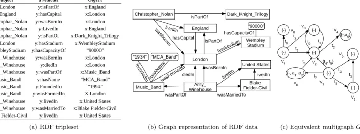
Prefixes: x= http://dbpedia.org/resource/ ; y=http://dbpedia.org/ontology/

Subject Predicate Object

x:London y:isPartOf x:England x:England y:hasCapital x:London x:Christophar_Nolan y:wasBornIn x:London x:Christophar_Nolan y:LivedIn x:England x:Christophar_Nolan y:isPartOf x:Dark_Knight_Trilogy

x:London y:hasStadium x:WembleyStadium x:WembleyStadium y:hasCapacityOf “90000” x:Amy_Winehouse y:wasBornIn x:London x:Amy_Winehouse y:diedIn x:London x:Amy_Winehouse y:wasPartOf x:Music_Band

x:Music_Band y:hasName “MCA_Band” x:Music_Band y:FoundedIn “1994” x:Music_Band y:wasFormedIn X:London x:Amy_Winehouse y:livedIn x:United States x:Amy_Winehouse y:wasMarriedTo x:Blake Fielder-Civil x:Blake Fielder-Civil y:livedIn x:United States

(a) RDF tripleset “MCA_Band” “1934” hasCapital isPartOf hasSta dium wasMarriedTo wasPartOf wasBornIn diedIn fo un de dIn _wasForm edIn hasA Nam e “90000” hasCapacityOf livedIn Blake Fielder-Civil United States Wembley Stadium Amy_ Winehouse London England Music_Band Christopher_Nolan wa_sB orn_In livedIn livedIn Dark_Knight_Trilogy isPartOf

(b) Graph representation of RDF data

{-} {-} {-, a₁, a₂} {-} {-,a₀} {-} {-} t₁ t₀ t₂ {t₄, t₅} t₆ t₇ t₈ V₀ V₂ V₁ V₃ V₄ V₅ V₆ {-} V₇ t₅ t₃ t₃ {-} V₈ t₀ t3 (c) Equivalent multigraph G

Figure 1: (a) RDF data in n-triple format; (b) graph representation (c) attributed multigraph G

deal with this problem, AMbER employs an efficient ap-proach that exploits structural properties of the multigraph query as well as the indices previously built on the multi-graph structure. Experimental evaluation over popular RDF benchmarks show the quality in terms of time performances and robustness of our proposal.

In this paper, we focus only on the SELECT/WHERE clause of the SPARQL language1_{, that constitutes the most}

impor-tant operation of any RDF query engines. It is out of the scope of this work to consider operators like FILTER, UNION and GROUP BY or manage RDF update. Such operations can be addressed in future as extensions of the current work. The paper is organized as follows. Section 2 introduces the basic notions about RDF and SPARQL language. In Sec-tion 3 AMbER is presented. SecSec-tion 4 describes the index-ing strategy while Section 5 presents the query processindex-ing. Related works are discussed in Section 6. Section 7 provides the experimental evaluation. Section 8 concludes.

2.

BACKGROUND AND PRELIMINARIES

In this section we provide basic definitions on the interplay between RDF and its multigraph representation. Later, we explain how the task of answering SPARQL queries can be reduced to multigraph homomorphism problem.

2.1

RDF Data

As per the W3C standards2_{, RDF data is represented as a}

set of triples <S, P, O>, as shown in Figure 1a, where each triple <s, p, o> consists of three components: a subject, a predicate and an object. Further, each component of the RDF triple can be of any two forms; an IRI (International-ized Resource Identifier) or a literal. For brevity, an IRI is usually written along with a prefix (e.g., <http://dbpedia.

1

http://www.w3.org/TR/sparql11-overview/

2_{http://www.w3.org/TR/2014/}

REC-rdf11-concepts-20140225/

org/resource/isPartOf> is written as ‘x:isPartOf’), whereas a literal is always written with inverted commas (e.g., “90000”). While a subject s and a predicate p are always an IRI, an object o is either an IRI or a literal.

RDF data can also be represented as a directed graph where, given a triple <s, p, o>, the subject s and the object o can be treated as vertices and the predicate p forms a directed edge from s to o, as depicted in Figure 1b. Further, to underline the difference between an IRI and a literal, we use standard rectangles and arc for the former while we use beveled corner and edge (no arrows) for the latter.

2.1.1

Data Multigraph Representation

Motivated by the graph representation of RDF data (Fig-ure 1b), we take a step further by transforming it to a data multigraph G, as shown in Figure 1c.

Let us consider an RDF triple <s, p, o> from the RDF triple-set <S, P, O>. Now to transform the RDF tripletriple-set into data multigraph G, we set four protocols: we always treat the subject s as a vertex; a predicate p is always treated as an edge; we treat the object o as a vertex only if it is an IRI (e.g., vertex v2corresponds to object ‘x:London’); when the

object is a literal, we combine the object o and the corre-sponding predicate p to form a tuple <p, o> and assign it as an attribute to the subject s (e.g., <‘y:hasCapacityOf’, “90000”> is assigned to vertex v4). Every vertex is assigned

a null value {-} in the attribute set. However, to realize this in the realms of graph management techniques, we main-tain three different dictionaries, whose elements are a pair of ‘key’ and ‘value’, and a mapping function that links them. The three dictionaries depicted in Table 2 are: a vertex dic-tionary (Table 2a), an edge-type dicdic-tionary (Table 2b) and an attribute dictionary (Table 2c). In all the three dictio-naries, an RDF entity represented by a ‘key’ is mapped to a corresponding ‘value’, which can be a vertex/edge/attribute identifier. Thus by using the mapping functions - Mv, Me,

respec-tively, we obtain a directed, vertex attributed data multi-graph G (Figure 1c), which is formally defined as follows.

Definition 1. Directed, Vertex Attributed Multigraph. A directed, vertex attributed multigraph G is defined as a 4-tuple (V, E, LV, LE) where V is a set of vertices, E ⊆

V × V is a set of directed edges with (v, v0) 6= (v0, v), LV is a

labelling function that assigns a subset of vertex attributes A to the set of vertices V , and LE is a labelling function that

assigns a subset of edge-types T to the edge set E.

To summarise, an RDF tripleset is transformed into a data multigraph G, whose elements are obtained by using the mapping functions as already discussed. Thus, the set of ver-tices V = {v0, . . . , vm} is the set of mapped subject/object

IRI, and the labelling function LV assigns a set of vertex

at-tributes A = {-, a0, . . . , an} (mapped tuple of predicate and

object-literal) to the vertex set V . The set of directed edges E is a set of pair of vertices (v, v0) that are linked by a pred-icate, and the labelling function LE assigns the set of edge

types T = {t0, . . . , tp} (mapped predicates) to these set of

edges. The edge set E maintains the topological structure of the RDF data. Further, mapping of object-literals and the corresponding predicates as a set of vertex attributes, results in a compact representation of the multigraph. For exam-ple (in Fig. 1c), all the object-literals and the corresponding predicates are reduced to a set of vertex attributes.

2.2

SPARQL Query

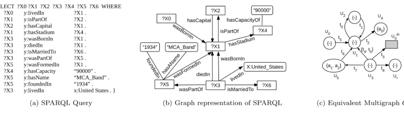
A SPARQL query usually contains a set of triple patterns, much like RDF triples, except that any of the subject, pred-icate and object may be a variable, whose bindings are to be found in the RDF data3_{. In the current work, we}

ad-dress the SPARQL queries with ‘SELECT/WHERE’ option, where the predicate is always instantiated as an IRI (Fig-ure 2a). The SELECT clause identifies the variables to appear in the query results while the WHERE clause provides triple patterns to match against the RDF data.

2.2.1

Query Multigraph Representation

In any valid SPARQL query (as in Figure 2a), every triplet has at least one unknown variable ?X, whose bindings are to be found in the RDF data. It should now be easy to observe that a SPARQL query can be represented in the form of a graph as in Figure 2b, which in turn is transformed into query multigraph Q (as in Figure 2c).

In the query multigraph representation, each unknown vari-able ?Xi is mapped to a vertex ui that forms the vertex

set U component of the query multigraph Q (e.g., ?X6 is

mapped to u6). Since a predicate is always instantiated as

an IRI, we use the edge-type dictionary in Table 2b, to map the predicate to an edge-type identifier ti∈ T (e.g.,

‘isMar-riedTo’ is mapped as t8). When an object oi is a literal,

we use the attribute dictionary (Table 2c), to find the at-tribute identifier ai for the predicate-object tuple <pi, oi>

(e.g., {a0} forms the attribute for vertex u4). Further, when

a subject or an object is an IRI, which is a not a variable, we

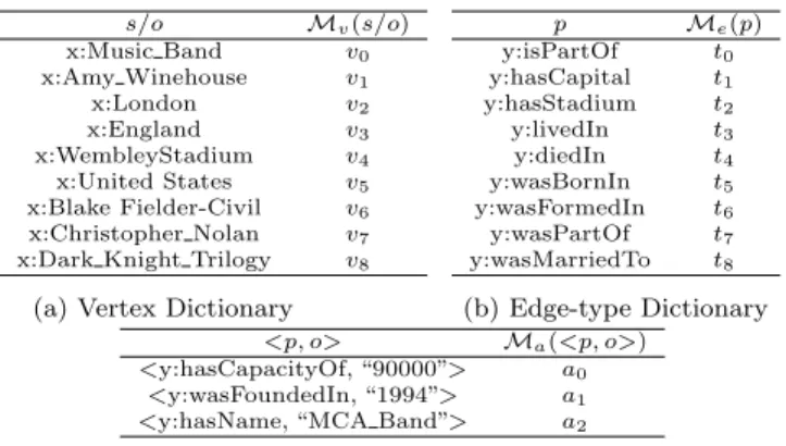
3_{http://www.w3.org/TR/2008/} REC-rdf-sparql-query-20080115/ s/o Mv(s/o) x:Music Band v0 x:Amy Winehouse v1 x:London v2 x:England v3 x:WembleyStadium v4 x:United States v5 x:Blake Fielder-Civil v6 x:Christopher Nolan v7 x:Dark Knight Trilogy v8

(a) Vertex Dictionary

p Me(p) y:isPartOf t0 y:hasCapital t1 y:hasStadium t2 y:livedIn t3 y:diedIn t4 y:wasBornIn t5 y:wasFormedIn t6 y:wasPartOf t7 y:wasMarriedTo t8 (b) Edge-type Dictionary <p, o> Ma(<p, o>) <y:hasCapacityOf, “90000”> a0 <y:wasFoundedIn, “1994”> a1 <y:hasName, “MCA Band”> a2

(c) Attribute Dictionary

Table 2: Dictionary look-up tables for vertices, edge-types and vertex attributes

use the vertex dictionary (2a), to map it to an IRI -vertex uirii (e.g., ‘x:United States’ is mapped to uiri0 ) and maintain

a set of IRI vertices R. Since this vertex is not a variable and a real vertex of the query, we portray it differently by a shaded square shaped vertex. When a query vertex uidoes

not have any vertex attributes associated with it (e.g., u0,

u1, u2, u3, u6), a null attribute {-} is assigned to it. On

the other hand, an IRI -vertex uirii ∈ R does not have any

attributes. Thus, a SPARQL query is transformed into a query multigraph Q.

In this work, we always use the notation V for the set of vertices of G, and U for the set of vertices of Q. Conse-quently, a data vertex v ∈ V , and a query vertex u ∈ U . Also, an incoming edge to a vertex is positive (default), and an outgoing edge from a vertex is labelled negative (‘-’).

2.3

SPARQL Querying by Adopting

Multigraph Homomorphism

As we recall, the problem of SPARQL querying is addressed by finding the solutions to the unknown variables ?X, that can be bound with the RDF data entities, so that the rela-tions (predicates) provided in the SPARQL query are re-spected. In this work, to harness the transformed data multigraph G and the query multigraph Q, we reduce the problem of SPARQL querying to a sub-multigraph homo-morphism problem. The RDF data is transformed into data multigraph G and the SPARQL query is transformed into query multigraph Q. Let us now recall that finding SPARQL answers in the RDF data is equivalent to finding all the sub-multigraphs of Q in G that are homomorphic. Thus, let us now formally introduce homomorphism for a vertex attributed, directed multigraph.

Definition 2. Sub-multigraph Homomorphism. Given a query multigraph Q = (U, EQ, LU, LQE) and a data

multi-graph G = (V, E, LV, LE), the sub-multigraph

homomor-phism from Q to G is a surjective function ψ : U → V such that:

1. ∀u ∈ U, LU(u) ⊆ LV(ψ(u))

2. ∀(um, un) ∈ EQ, ∃ (ψ(um), ψ(un)) ∈ E, where (um, un)

SELECT ?X0 ?X1 ?X2 ?X3 ?X4 ?X5 ?X6 WHERE { ?X0 y:livedIn ?X1 . ?X1 y:isPartOf ?X2 . ?X2 y:hasCapital ?X1 . ?X1 y:hasStadium ?X4 . ?X3 y:wasBornIn ?X1 . ?X3 y:diedIn ?X1 . ?X3 y:isMarriedTo ?X6 . ?X3 y:wasPartOf ?X5 . ?X5 y:wasFormedIn ?X1 . ?X4 y:hasCapacity “90000” . ?X5 y:hasName “MCA_Band” . ?X5 y:foundedIn “1934” . ?X3 y:livedIn x:United States . }

(a) SPARQL Query

“MCA_Band” “1934” hasCapital isPartOf hasStadium isMarriedTo wasPartOf wasBornIn diedIn fo un de dIn _wasForm edIn hasA Nam e “90000” hasCapacityOf X:United_States livedIn was Born_In ?X6 ?X1 ?X2 ?X3 ?X5 ?X0 ?X4

(b) Graph representation of SPARQL

{-} {-} {a₁, a₂} {-} {-} t₁ t₀ t₂ {t₄, t₅} t₆ t₇ t₈ U₃ U₅ U₁ U_{2 U} 4 U6 {a₀} {-} U₀ t₅ U₀iri t₃ (c) Equivalent Multigraph Q

Figure 2: (a) SPARQL query representation; (b) graph representation (c) attributed multigraph Q

Thus, by finding all the sub-multigraphs in G that are ho-momorphic to Q, we enumerate all possible hoho-momorphic embeddings of Q in G. These embeddings contain the solu-tion for each of the query vertex that is an unknown variable. Thus, by using the inverse mapping function M−1v (vi)

(in-troduced already), we find the bindings for the SPARQL query. The decision problem of subgraph homomorphism is NP-complete. This standard subgraph homomorphism problem can be seen as a particular case of sub-multigraph homomorphism, where both the labelling functions LE and

LQ_E always return the same subset of edge-types for all the edges in both Q and G. Thus the problem of sub-multigraph homomorphism is at least as hard as subgraph homomor-phism. Further, the subgraph homomorphism problem is a generic scenario of subgraph isomorphism problem where, the injectivity constraints are slackened [10].

3.

AMBER: A SPARQL QUERYING ENGINE

Now we present an overview of our proposal AMbER (At-tributed Mulitgraph Based Engine for RDF querying). AMbER encompasses two different stages: an offline stage during which, RDF data is transformed into multigraph G and then a set of index structures I is constructed that captures the necessary information contained in G; an online step dur-ing which, a given SPARQL query is transformed into a multigraph Q, and then by exploiting the subgraph match-ing techniques along with the already built index structures I, the homomorphic matches of Q in G are obtained. Given a multigraph representation Q of a SPARQL query, AMbER decomposes the query vertices U into a set of core vertices Uc and satellite vertices Us. Intuitively, a vertex

u ∈ U is a core vertex, if the degree of the vertex is more than one; on the other hand, a vertex u with degree one is a satellite vertex. For example, in Figure 2c, Uc= {u1, u3, u5}

and Us = {u0, u2, u4, u6}. Once decomposed, we run the

sub-multigraph matching procedure on the query structure spanned only by the core vertices. However, during the pro-cedure, we also process the satellite vertices (if available) that are connected to a core vertex that is being processed. For example, while processing the core vertex u1 , we also

process the set of satellite vertices {u0, u2, u4} connected to

it; whereas, the core vertex u5 has no satellite vertices to

be processed. In this way, as the matching proceeds, the entire structure of the query mulitgraph Q is processed to

find the homomorphic embeddings in G. The set of indexing structures I are extensively used during the process of sub-multigraph macthing. The homomorphic embeddings are finally translated back to the RDF entities using the inverse mapping function M−1v as discussed in Section 2.

4.

INDEX CONSTRUCTION

Given a data multigraph G, we build the following three different indices: (i) an inverted list A for storing the set of data vertex for each attribute in ai ∈ A (ii) a trie index

structure S to store features of all the data vertices V (iii) a set of trie index structures N to store the neighbourhood information of each data vertex v ∈ V . For brevity of rep-resentation, we ensemble all the three index structures into I := {A, S, N }.

During the query matching procedure (the online step), we access these indexing structures to obtain the candidate so-lutions for a query vertex u. Formally, for a query ver-tex u, the candidate solutions are a set of data vertices Cu = {v|v ∈ V } obtained by accessing A or S or N ,

de-noted as CuA, C S u and C N u respectively.

4.1

Attribute Index

The set of vertex attributes is given by A = {a0, . . . , an}

(Section 2), where a data vertex v ∈ V might have a subset of A assigned to it. We now build the vertex attribute index A by creating an inverted list where a particular attribute aihas the list of all the data vertices in which it appears.

Given a query vertex u with a set of vertex attributes u.A ⊆ A, for each attribute ai∈ u.A, we access the index structure

A to fetch a set of data vertices that have ai. Then we find a

common set of data vertices that have the entire attribute set u.A. For example, considering the query vertex u5(Fig. 2c),

it has an attribute set {a1, a2}. The candidate solutions for

u5 are obtained by finding all the common data vertices, in

A, between a1 and a2, resulting in CuA5 = {v0}.

4.2

Vertex Signature Index

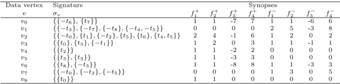
The index S captures the edge type information from the data vertices. For a lucid understanding of this indexing schema we formally introduce the notion of vertex signature that is defined for a vertex v ∈ V , which encapsulates the edge information associated with it.

Data vertex Signature Synopses v σv f1+ f + 2 f + 3 f + 4 f − 1 f − 2 f − 3 f − 4 v0 {{−t6}, {t7}} 1 1 -7 7 1 1 -6 6 v1 {{−t3}, {−t7}, {−t8}, {−t4, −t5}} 0 0 0 0 2 5 -3 8 v2 {{−t0}, {t1}, {−t2}, {t5}, {t6}, {t4, t5}} 2 4 -1 6 1 2 0 2 v3 {{t0}, {t3}, {−t1}} 1 2 0 3 1 1 -1 1 v4 {{t2}} 1 1 -2 2 0 0 0 0 v5 {{t3}, {t3}} 1 1 -3 3 0 0 0 0 v6 {{t8}, {−t3}} 1 1 -8 8 1 1 -3 3 v7 {{−t0}, {−t3}, {−t5}} 0 0 0 0 1 3 0 5 v8 {{t0}} 1 1 0 0 0 0 0 0

Table 3: Vertex signatures and the corresponding synopses for the vertices in the data multigraph G (Figure 1c)

Definition 3. Vertex signature. For a vertex v ∈ V , the vertex signature σv is a multiset containing all the

di-rected multi-edges that are incident on v, where a multi-edge between v and a neighbouring vertex v0 is represented by a set that corresponds to the edge types. Formally, σv =

S

v0∈N (v)LE(v, v0) where N (v) is the set of neighbourhood

vertices of v, and ∪ is the union operator for multiset. The index S is constructed by tailoring the information sup-plied by the vertex signature of each vertex in G. To extract some interesting features, let us observe the vertex signature σv2 as supplied in Table 3. To begin with, we can represent

the vertex signature σv2 separately for the incoming and

outgoing multi-edges as σ+v2= {{t1}, {t5}, {t6}, {t4, t5}} and

σ−v2 = {{−t0}{−t2}} respectively. Now we observe that σ

+ v2

has four distinct multi-edges and σv−2has two distinct

multi-edges. Now, lets think that we want find candidate solutions for a query vertex u. The data vertex v2can be a match for

u only if the signature of u has at most four incoming (‘+’) edges and at most two outgoing (‘-’) edges; else v2 can not

be a match for u. Thus, more such features (e.g., maximum cardinality of a set in the vertex signature) can be proposed to filter out irrelevant candidate vertices. Thus, for each ver-tex v, we propose to extract a set of features by exploiting the corresponding vertex signature. These features consti-tute a synopses, which is a surrogate representation that approximately captures the vertex signature information. The synopsis of a vertex v contains a set of features F , whose values are computed from the vertex signature σv. In this

background, we propose four distinct features: f1- the

max-imum cardinality of a set in the vertex signature; f2 - the

number of unique dimensions in the vertex signature; f3

-the minimum index value of -the edge type; f4 - the

maxi-mum index value of the edge type. For f3 and f4, the index

values of edge type are nothing but the position of the se-quenced alphabet. These four basic features are replicated separately for outgoing (negative) and incoming (positive) edges, as seen in Table 3. Thus for the vertex v2, we obtain

f₁+ = 2, f₂+ = 4, f₃+ = −1 and f₄+ = 7 for the incoming edge set and f1−= 1, f

− 2 = 2, f − 3 = 0 and f − 4 = 2 for the

outgoing edge set. Synopses for the entire vertex set V for the data multigraph G are depicted in Table 3.

Once the synopses are computed for all data vertices, an R-tree is constructed to store all the synopses. This R-tree constitutes the vertex signature index S. A synopsis with |F | fields forms a leaf in the R-tree.

When a set of possible candidate solutions are to be obtained for a query vertex u, we create a vertex signature σu in

order to compute the synopsis, and then obtain the possible solutions from the R-tree structure.

The general idea of using an R-tree is as follows. A synopsis F of a data vertex spans an axes-parallel rectangle in an |F |-dimensional space, where the maximum co-ordinates of the rectangle are the values of the synopses fields (f1, . . . , f|F |),

and the minimum co-ordinates are the origin of the rectangle (filled with zero values). For example, a data vertex repre-sented by a synopses with two features F (v) = [2, 3] spans a rectangle in a 2-dimensional space in the interval range ([0, 2], [0, 3]). Now, if we consider synopses of two query ver-tices, F (u1) = [1, 3] and F (u2) = [1, 4], we observe that the

rectangle spanned by F (u1) is wholly contained in the

rect-angle spanned by F (v) but F (u2) is not wholly contained in

F (v). Thus, u1is a candidate match while u2is not.

Lemma 1. Querying the vertex signature index S con-structed with synopses, guarantees to output at least the en-tire set of candidate solutions.

Proof. Consider the field f1± in the synopses that

rep-resents the maximum cardinality of the neighbourhood sig-nature. Let σu be the signature of the query vertex u and

{σv1, . . . , σvn} be the set of signatures on the data vertices.

By using f1 we need to show that CuS has at least all the

valid candidate matches. Since we are looking for a superset of query vertex signature, and we are checking the condition f1±(u) ≤ f

±

1 (vi), where vi ∈ V , a vertex vi is pruned if it

does not match the inequality criterion since, it can never be an eligible candidate. This analogy can be extended to the entire synopses, since it can be applied disjunctively.

Formally, the candidates solutions for a vertex u can be writ-ten as CuS = {v|∀i∈[1,...,|F |]f

± i (u) ≤ f

±

i (v)}, where the

con-straints are met for all the |F |-dimensions. Since we apply the same inequality constraint to all the fields, we negate the fields that refer to the minimal index value of the edge type (f+

3 and f −

3 ) so that the rectangular containment problem

still holds good. Further to respect the rectangular con-tainment, we populate the synopses fields with ‘0’ values, in case, the signature does not have either positive or negative edges in it, as seen for v1, v3, v4, v5 and v7.

For example, if we want to compute the possible candidates for a query vertex u0 in Figure 2c, whose signature is σu0=

{−t5}, we compute the synopsis which is [0 0 0 0 1 1 5 5].

in the R-tree, whose elements are depicted in Table 3, which gives us the candidate solutions CuS0= {v1, v7}, thus pruning

the rest of the vertices.

The S index helps to prune the vertices that do not respect the edge type constraints. This is crucial since this pruning is performed for the initial query vertex, and hence many candidates are cast away, thereby avoiding unnecessary re-cursion during the matching procedure. For example, for the initial query vertex u0, whose candidate solutions are

{v1, v7}, the recursion branch is run only on these two

start-ing vertices instead of the entire vertex set V .

4.3

Vertex Neighbourhood Index

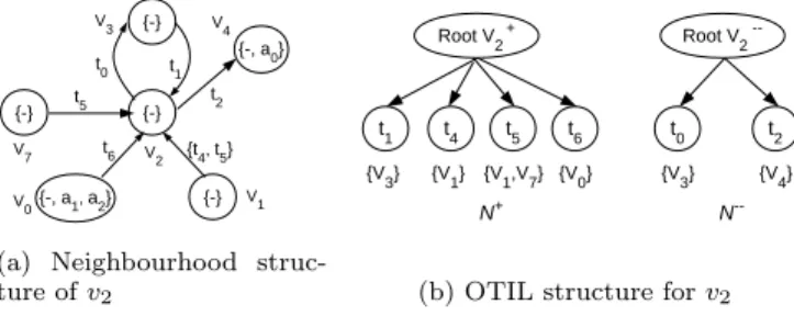
The vertex veighbourhood index N captures the topological structure of the data multigraph G. The index N comprises of 1-neighbourhood trees built for each data vertex v ∈ V . Since G is a directed multigraph, and each vertex v ∈ V can have both the incoming and outgoing edges, we construct two separate index structures N+and N−for incoming and outgoing edges respectively, that constitute the structure N . To understand the index structure, let us consider the data vertex v2from Figure 1c, shown separately in Figure 3a. For

this vertex v2, we collect all the neighbourhood information

(vertices and multi-edges), and represent this information by a tree structure, built separately for incoming (‘+’) and out-going (‘-’) edges. Thus, the tree representation of a vertex v contains the neighbourhood vertices and the corresponding multi-edges, as shown in Figure 3b, where the vertices of the tree structure are represented by the edge types.

{-} {-} {-, a₁, a₂} {-} {-, a₀} t₁ t₀ t₂ {t₄, t₅} t₆ V₀ V₂ V₁ V₃ V₄ {-} V₇ t₅

(a) Neighbourhood struc-ture of v2 t₀ Root V₂+ t₁ t₄ t₅ t₆ t₂ Root V₂ --{V₃} {V₁} {V₁,V₇} {V₀} {V₃} {V₄} N+ _N

--(b) OTIL structure for v2

Figure 3: Building Neighbourhood Index for data vertex v2

In order to construct an efficient tree structure, we take inspiration from [13] to propose the structure - Ordered Trie with Inverted List (OTIL). To construct the OTIL index as shown in Figure 3b, we insert each ordered multi-edge that is incident on v at the root of the trie. Consider a data vertex vi, with a set of n neighbourhood vertices N (vi).

Now, for every pair of incoming edge (vi, Nj(vi)), where

j ∈ {1, . . . , n}, there exists a multi-edge {ti, . . . , tj}, which

is inserted into the OTIL structure N+_{. Similarly for every}

pair of outgoing edge (Nj(vi), vi), there exists a multi-edge

{tm, . . . , tn}, which is inserted into the OTIL structure N−

maintaining two OTIL structures that constitute N . Each multi-edge is ordered (w.r.t. increasing edge type indexes), before inserting into the respective OTIL structure, and the order is universally maintained for all data vertices. Further, for every edge type ti, we maintain a list that contains all

the neighbourhood vertices N+(vi)/N−(vi), that have the

edge type ti incident on them.

{-} {-} {a₁, a₂} {-} {-} t₁ t₀ t₂ {t₄, t₅} t₆ t₇ t₈ U₃ U₅ U₁ U₂ U₄ U6 {a₀} {-} U₀ t₅

(a) Query graph Q highlighted with satellite vertices

{-} {-} {a₁, a₂} {t₄, t₅} t₆ t₇ U₃ U₅ U₁

(b) Query graph spanned by core vertices

Figure 4: Decomposing the query multigraph into core and satellite vertices

To understand the utility of N , let us consider an illustrative example. Considering the query multigraph Q in Figure 2c, let as assume that we want to find the matches for the query vertices u1 and u0 in order. Thus, for the initial vertex u1,

let us say, we have found the set of candidate solutions which is {v2}. Now, to find the candidate solutions for the next

query vertex u0, it is important to maintain the structure

spanned by the query vertices, and this is where the index-ing structure N is accessed. Thus to retain the structure of the query multigraph (in this case, the structure between u1 and u0), we have to find the data vertices that are in

the neighbourhood of already matched vertex v2 (a match

for vertex u1), that has the same structure (edge types)

be-tween u1 and u0 in the query graph. Thus to fetch all the

data vertices that have the edge type t5, which is directed

towards v2 and hence ‘+’, we access the neighbourhood

in-dex trie N+_{for vertex v}

2, as shown in Figure 3. This gives

us a set of candidate solutions CuN0 = {v1, v7}. It is easy to

observe that, by maintaining two separate indexing struc-tures N+ _{and N}−

, for both incoming and outgoing edges, we can reduce the time to fetch the candidate solutions. Thus, in a generic scenario, given an already matched data vertex v, the edge direction ‘+’ or ‘-’, and the set of edge types T0⊆ T , the index N will find a set of neighbourhood data vertices {v0|(v0, v) ∈ E ∧ T0 ⊆ LE(v0, v)} if the edge

direction is ‘+’ (incoming), while N returns {v0|(v, v0) ∈ E ∧ T0⊆ LE(v, v0)} if the edge direction is ‘-’ (outgoing).

5.

QUERY MATCHING PROCEDURE

In order to follow the working of the proposed query match-ing procedure, we formalize the notion of core and satellite vertices. Given a query graph Q, we decompose the set of query vertices U into a set of core vertices Uc and a set of

satellite vertices Us. Formally, when the degree of the query

graph ∆(Q) > 1, Uc = {u|u ∈ U ∧ deg(u) > 1}; however,

when ∆(Q) = 1, i.e, when the query graph is either a vertex or a multiedge, we choose one query vertex at random as a core vertex, and hence |Uc|= 1. The remaining vertices are

classified as satellite vertices, whose degree is always 1. For-mally, Us= {U \ Uc}, where for every u ∈ Us, deg(u) = 1.

The decomposition for the query multigraph Q is depicted in Figure 4, where the satellite vertices are separated (ver-tices under the shaded region in Fig. 4a), in order to obtain the query graph that is spanned only by the core vertices (Fig. 4b).

The proposed AMbER-Algo (Algorithm 3) performs recur-sive sub-multigraph matching procedure only on the query structure spanned by Uc as seen in Figure 4b. Since the

entire set of satellite vertices Us is connected to the query

structure spanned by the core vertices, AMbER-Algo pro-cesses the satellite vertices while performing sub-multigraph matching on the set of core vertices. Thus during the re-cursion, if the current core vertex has satellite vertices con-nected to it, the algorithm retrieves directly a list of possible matching for such satellite vertices and it includes them in the current partial solution. Each time the algorithm exe-cutes a recursion branch with a solution, the solution not only contains a data vertex match vc for each query vertex

belonging to Uc, but also a set of matched data vertices Vs

for each query vertex belonging to Us. Each time a

solu-tion is found, we can generate not only one, but a set of embeddings through the Cartesian product of the matched elements in the solution.

Since finding SPARQL solutions is equivalent to finding momorphic embeddings of the query multigraph, the ho-momorphic matching allows different query vertices to be matched with the same data vertices. Recall that there is no injectivity constraint in sub-multigraph homomorphism as opposed to sub-multigraph isomorphism [10]. Thus dur-ing the recursive matchdur-ing procedure, we do not have to check if the potential data vertex has already been matched with previously matched query vertices. This is an advan-tage when we are processing satellite vertices: we can find matches for each satellite vertex independently without the necessity to check for a repeated data vertex.

Before getting into the details of the AMbER-Algo, we first explain how a set of candidate solutions is obtained when there is information associated only with the vertices. Then we explain how a set of candidate solutions is obtained when we encounter the satellite vertices.

5.1

Vertex Level Processing

To understand the generic query processing, it is necessary to understand the matching process at vertex level. When-ever a query vertex u ∈ U is being processed, we need to check if u has a set of attributes A associated with it or any IRI s are connected to it (recall Section 2.2).

Algorithm 1: ProcessVertex(u, Q, A, N ) 1 if u.A 6= ∅ then 2 CA u = QueryAttIndex(A, u.A) 3 if u.R 6= ∅ then 4 CI u= T

uiri_i ∈u.R( QueryNeighIndex(N , L Q E(u, u

iri i ), uirii ) ) 5 CandAttu= CAu ∩ CIu /* Find common candidates */ 6 return CandAttu

To process an arbitrary query vertex, we propose a proce-dure ProcessVertex, depicted in Algorithm 1. This algo-rithm is invoked only when a vertex u has at least, either a set of vertex attributes or any IRI associated with it. The ProcessVertex procedure returns a set of data vertices CandAttu, which are matchable with u; in case CandAttu

is empty, then the query vertex u has no matches in V . As seen in Lines 1-2, when a query vertex u has a set of

{-} {-} t₁ t₀ t₂ U₄ {a₀} {-} U₀ t₅ U₁ U₂

Figure 5: A star structure in the query multigraph Q

vertex attributes i.e., u.A 6= ∅, we obtain the candidate so-lutions CA

u by invoking QueryAttIndex procedure, that

accesses the index A as explained in Section 4.1. For exam-ple, the query vertex u5with vertex attributes {a1, a2}, can

only be matched with the data vertex v0; thus CuA5= {v0}.

When a query vertex u has IRI s associated with it, i.e., u.R 6= ∅ (Lines 3-4), we find the candidate solutions CuI by

invoking the QueryNeighIndex procedure. As we recall from Section 2.2, a vertex u is connected to an IRI vertex uirii through a multi-edge L

Q E(u, u

iri

i ). An IRI vertex uirii

always has only one data vertex v, that can match. Thus, the candidate solutions CuI are obtained by invoking the

QueryNeighIndex procedure, that fetches all the neigh-bourhood vertices of v that respect the multi-edge LQ_E(u, uiri

i ).

The procedure is invoked until all the IRI vertices u.R are processed (Line 4). Considering the example in Figure 2c, u3 is connected to an IRI -vertex uiri0 , which has a unique

data vertex match v5, through the multi-edge {−t3}. Using

the neighbourhood index N , we look for the neighbourhood vertices of v5, that have the multi-edge {−t3}, which gives

us the candidate solutions CI

u3= {v1}.

Finally in Line 5, the merge operator ∩ returns a set of common candidates CandAttu, only if u.A 6= ∅ and u.R 6= ∅.

Otherwise, CuA or C I

uare returned as CandAttu.

5.2

Processing Satellite Vertices

In this section, we provide insights on processing a set of satellite vertices Usat ⊆ Us that are connected to a core

vertex uc ∈ Uc. This scenario results in a structure that

appears frequently in SPARQL queries called star structure [7, 9].

A typical star structure depicted in Figure 5, has a core ver-tex uc= u1, and a set of satellite vertices Usat= {u0, u2, u4}

connected to the core vertex. For each candidate solution of the core vertex u1, we process u0, u2, u4 independently of

each other, since there is no structural connectivity (edges) among them, although they are only structurally connected to the core vertex u1.

Lemma 2. For a given star structure in a query graph, each satellite vertex can be independently processed if a can-didate solution is provided for the core vertex uc.

Proof. Consider a core vertex uc that is connected to

a set of satellite vertices Usat = {u0, . . . , us}, through a

set of edge-types T0 = {t0, . . . , ts}. Let us assume vc is

a candidate solution for the core vertex uc, and we want

where i 6= j. Now, the candidate solutions for ui and uj

can be obtained by fetching the neighbourhoods of already matched vertex vc that respect the edge-type ti ∈ T0 and

tj ∈ T0 respectively. Since two satellite vertices ui and uj

are never connected to each other, the candidate solutions of uiare independent of that of uj. This analogy applies to

all the satellite vertices.

Algorithm 2: MatchSatVertices(A, N , Q, Usat, vc)

1 Set: Msat= ∅, where Msat= {[us, Vs]}|Usat|_s=1 2 for all us∈ Usatdo

3 Cand_us = QueryNeighIndex(N , LQE(uc, us), vc) 4 Cand_us = Cand_{us∩ ProcessVertex(us}, Q, A, N ) 5 if Cand_us6= ∅ then

6 Msat= Msat∪ (us, Candus) /* Satellite solutions */

7 else

8 return Msat:= 0 /* No solutions possible */

9 return Msat /* Matches for satellite vertices */

Given a core vertex uc, we initially find a set of candidate

solutions Canduc, by using the index S. Then, for each

candidate solution vc ∈ Canduc, the set of solutions for all

the satellite vertices Usat that are connected to uc are

re-turned by the MatchSatVertices procedure, described in Algorithm 2. The set of solution tuple Msatdefined in Line

1, stores the candidate solutions for the entire set of satel-lite vertices Usat. Formally, Msat = {[us, Vs]}

|Usat|

s=1 , where

us ∈ Usat and Vs is a set of candidate solutions for us.

In order to obtain candidate solutions for us, we query the

neighbourhood index N (Line 3); the QueryNeighIndex function obtains all the neighbourhood vertices of already matched vc, that also considers the multi-edge in the query

multigraph LQ_E(uc, us). As every query vertex us ∈ Usat

is processed, the solution set Msat that contains candidate

solutions grows until all the satellite vertices have been pro-cessed (Lines 2-8).

In Line 4, the set of candidate solutions Candus are refined

by invoking Algorithm 1 (VertexProcessing). After the refinement, if there are finite candidate solutions, we up-date the solution Msat; else, we terminate the procedure as

there can be no matches for a given matched vertex vc. The

MatchSatVertices procedure performs two tasks: firstly, it checks if the candidate vertex vc ∈ Candus is a valid

matchable vertex and secondly, it obtains the solutions for all the satellite vertices.

5.3

Arbitrary Query Processing

Algorithm 3 shows the generic procedure we develop to pro-cess arbitrary queries.

Recall that for an arbitrary query Q, we define two different types of vertexes: a set of core vertices Ucand a set of

satel-lite vertices Us. The QueryDecompose procedure in Line

1 of Algorithm 3, performs this decomposition by splitting the query vertices U into Ucand Us, as observed in Figure 4.

To process arbitrary query multigraphs, we perform recur-sive sub-mulitgraph matching procedure on the set of core vertices Uc⊆ U ; during the recursion, satellite vertexes

con-nected to a specific core vertex are processed too. Since the

recursion is performed on the set of core vertices, we propose a few heuristics for ordering the query vertices.

Ordering of the query vertices forms one of the vital steps for subgraph matching algorithms [10]. In any subgraph matching algorithm, the embeddings of a query subgraph are obtained by exploring the solution space spanned by the data graph. But since the solution space itself can grow exponentially in size, we are compelled to use intelligent strategies to traverse the solution space. In order to achieve this, we propose a heuristic procedure VertexOrdering (Line 2, Algorithm 3) that employs two ranking functions. The first ranking function r1 relies on the number of

satel-lite vertices connected to the core vertex, and the query ver-tices are ordered with the decreasing rank value. Formally, r1(u) = |Usat|, where Usat= {us|us∈ Us∧ (u, us) ∈ E(Q)}.

A vertex with more satellite vertices connected to it, is rich in structure and hence it would probably yield fewer can-didate solutions to be processed under recursion. Thus, in Figure 4, u1is chosen as an initial vertex. The second

rank-ing function r2 relies on the number of incident edges on

a query vertex. Formally, r2(u) = Pm_j=1|σ(u)j|, where u

has m multiedges and |σ(u)j| captures the number of edge types in the jth_{multiedge. Again, U}ord

c contains the ordered

vertices with the decreasing rank value r2. Further, when

there are no satellite vertices in the query Q, this ranking function gets the priority. Despite the usage of any rank-ing function, the query vertices in Ucord, when accessed in

sequence, should be structurally connected to the previous set of vertices. If two vertices tie up with the same rank, the rank with lesser priority determines which vertex wins. Thus, for the example in Figure 4, the set of ordered core vertices is Uord

c = {u1, u3, u5}.

Algorithm 3: AMbER-Algo (I, Q)

1 QueryDecompose: Split U into Ucand Us 2 Uord

c = VertexOrdering(Q, Uc) 3 uinit= u|u ∈ U_cord

4 CandInit = QuerySynIndex(uinit, S)

5 CandInit = CandInit ∩ ProcessVertex(uinit, Q, A, N ) 6 Fetch: Uinitsat = {u|u ∈ Us∧ (uinit, u) ∈ E(Q)} 7 Set: Emb = ∅

8 for vinit∈ CandInit do 9 Set: M = ∅, Ms= ∅, Mc= ∅

10 if Usat

init6= ∅ then

11 Msat= MatchSatVertices(A, N , Q, Uinitsat, vinit)

12 if Msat6= ∅ then

13 for [us, Vs] ∈ Msatdo

14 Update: Ms= Ms∪ [us, Vs]

15 Update: Mc= Mc∪ [uinit, vinit]

16 Emb = Emb ∪ HomomorphicMatch(M, I, Q, Ucord)

17 else

18 Update: Mc= Mc∪ (uinit, vinit)

19 Emb = Emb ∪ HomomorphicMatch(M, I, Q, Ucord) 20 return Emb /* Homomorphic embeddings of query multigraph */

The first vertex in the set Uord

c is chosen as the initial vertex

uinit (Line 3), and subsequent query vertices are chosen in

sequence. The candidate solutions for the initial query ver-tex CandInit are returned by QuerySynIndex procedure (Line 4), that are constrained by the structural properties (neighbourhood structure) of uinit. By querying the index

so-lutions CandInit ∈ V that match the structure (multiedge types) associated with uinit. Although some candidates in

CandInit may be invalid, all valid candidates are present in CandInit, as deduced in Lemma 1. Further, ProcessVer-tex procedure is invoked to obtain the candidates solutions according to vertex attributes and IRI information, and then only the common candidates are retained.

Before getting into the details of the algorithm, we explain how the solutions are handled and how we process each query vertex. We define M as a set of tuples, whose ith

tuple is represented as Mi= [mc, Ms], where mcis a

solu-tion pair for a core vertex, and Msis a set of solution pairs

for the set of satellite vertices that are connected to the core vertex. Formally, mc= (uc, vc), where ucis the core vertex

and vcis the corresponding matched vertex; Ms is a set of

solution pairs, whose jth_{element is a solution pair (u} s, Vs),

where usis a satellite vertex and Vsis a set of matched

ver-tices. In addition, we maintain a set Mcwhose elements are

the solution pairs for all the core vertices. Thus during each recursion branch, the size of M grows until it reaches the query size |U |; once |M |= |U |, homomorphic matches are obtained.

For all the candidate solutions of initial vertex CandInit, we perform recursion to obtain homomorphic embeddings (lines 8-19). Before getting into recursion, for each initial match vinit ∈ CandInit, if it has satellite vertices connected to

it, we invoke the MatchSatVertices procedure (Lines 10-11). This step not only finds solution matches for satellite vertices, if there are, but also checks if vinit is a valid

can-didate vertex. If the returned solution set Msat is empty,

then vinit is not a valid candidate and hence we continue

with the next vinit∈ CandInit; else, we update the set of

solution pairs Ms for satellite vertices and the solution pair

Mcfor the core vertex (Lines 12-15) and invoke

Homomor-phicMatch procedure (Lines 17). On the other hand, if there are no satellite vertices connected to uinit, we update

the core vertex solution set Mc and invoke

Homomorphic-Match procedure (Lines 18-19).

Algorithm 4: HomomorphicMatch(M, I, Q, Ucord)

1 if |M |= |U | then

2 return GenEmb(M )

3 Emb = ∅

4 Fetch: unxt= u|u ∈ Uord c 5 Nq= {uc|uc∈ Mc} ∩ adj(unxt)

6 Ng= {vc|vc∈ Mc∧ (uc, vc) ∈ Mc}, where uc∈ Nq 7 Cand_unxt=T|Nq |_n=1(QueryNeighIndex(N , LQ_E(un, unxt), vn)) 8 Cand_unxt= Cand_unxt∩ ProcessVertex(unxt, Q, A, N ) 9 for each vnxt∈ Cand_unxtdo

10 Fetch: Unxtsat= {u|u ∈ Vs∧ (unxt, u) ∈ E(Q)}

11 if Usat

nxt6= ∅ then

12 Msat= MatchSatVertices(A, N , Q, Unxtsat, vnxt)

13 if Msat6= ∅ then

14 for every [us_{, V}s_{] ∈ M} satdo

15 Update: Ms= Ms∪ [us, Vs]

16 Update: Mc= Mc∪ (unxt, vnxt)

17 Emb = Emb ∪ HomomorphicMatch(M, I, Q, Ucord)

18 else

19 Update: Mc= Mc∪ (unxt, vnxt)

20 Emb = Emb ∪ HomomorphicMatch(M, I, Q, Uord

c )

21 return Emb

In the HomomorphicMatch procedure (Algorithm 4), we fetch the next query vertex from the set of ordered core vertices Ucord(Line 4). Then we collect the neighbourhood

vertices of already matched core query vertices and the cor-responding matched data vertices (Lines 5-6). As we recall, the set Mcmaintains the solution pair mc= (uc, vc) of each

matched core query vertex. The set Nq collects the already

matched core vertices uc ∈ Mc that are also in the

neigh-bourhood of unxt, whose matches have to be found.

Fur-ther, Ng contains the corresponding matched query vertices

vc∈ Mc. As the recursion proceeds further, we can find only

those matchable data vertices of unxt that are in the

neigh-bourhood of all the matched vertices v ∈ Ng, so that the

query structure is maintained. In Line 7, for each un∈ Nq

and the corresponding vn ∈ Ng, we query the

neighbour-hood index N , to obtain the candidate solutions Candunxt,

that are in the neighbourhood of already matched data ver-tex vn and have the multiedge LQE(un, unxt), obtained from

the query multigraph Q. Finally (line 7), only the set of candidates solutions that are common for every un∈ Nqare

retained in Candunxt.

Further, the candidate solutions are refined with the help of ProcessVertex procedure (Line 8). Now, for each of the valid candidate solution vnxt ∈ Candunxt, we recursively

call the HomomorphicMatch procedure. When the next query vertex unxthas no satellite vertices attached to it, we

update the core vertex solution set Mcand call the recursion

procedure (Lines 19-20). But when unxthas satellite vertices

attached to it, we obtain the candidate matches for all the satellite vertices by invoking the MatchSatVertices pro-cedure (Lines 11-12); if there are matches, we update both the satellite vertex solution Msand the core vertex solution

Mc, and invoke the recursion procedure (Line 17).

Once all the query vertices have been matched for the cur-rent recursion step, the solution set M contains the solu-tions for both core and satellite vertices. Thus when all the query vertices have been matched, we invoke the Gen-Emb function (Line 2) which returns the set of embeddings, that are updated in Emb. The GenEmb function treats the solution vertex vc of each core vertex as a singleton

and performs Cartesian product among all the core vertex singletons and satellite vertex sets. Formally, Embpart =

{v1

c} × . . . × {v |Uc|

c } × Vs1× . . . × V |Us|

c . Thus, the partial set

of embeddings Embpartis added to the final result Emb.

6.

RELATED WORK

The proliferation of semantic web technologies has influ-enced the popularity of RDF as a standard to represent and share knowledge bases. In order to efficiently answer SPARQL queries, many stores and API inspired by rela-tional model were proposed [6, 3, 12, 5]. x-RDF-3X [12], inspired by modern RDBMS, represent RDF triples as a big three-attribute table. The RDF query processing is boosted using an exhaustive indexing schema coupled with statistics over the data. Also Virtuoso[6] heavily exploits RDBMS mechanism in order to answer SPARQL queries. Virtuoso is a column-store based systems that employs sorted multi-column multi-column-wise compressed projections. Also these sys-tems build table indexing using standard B-trees. Jena [5] supplies API for manipulating RDF graphs. Jena ex-ploits multiple-property tables that permit multiple views

of graphs and vertices which can be used simultaneously. Recently, the database community has started to investi-gate RDF stores based on graph data management tech-niques [15, 10]. gStore [15] applies graph pattern matching using the filter-and-refinement strategy to answer SPARQL queries. It employs an indexing schema, named VS∗-tree, to concisely represent the RDF graph. Once the index is built, it is used to find promising subgraphs that match the query. Finally, exact subgraphs are enumerated in the refinement step. Turbo Hom++ [10] is an adaptation of a state of the art subgraph isomorphism algorithm (TurboISO[8]) to the

problem of SPARQL queries. Starting from the standard graph isomorphism problem, the authors relax the injectiv-ity constraint in order to handle the graph homomorphism, which is the RDF pattern matching semantics.

Unlike our approach, TurboHom++ does not index the RDF

graph, while gStore concisely represents RDF data through VS∗-tree. Another difference between AMbER and the other graph stores is that our approach explicitly manages the multigraph induced by the SPARQL queries while no clear discussion is supplied for the other tools.

7.

EXPERIMENTAL ANALYSIS

In this section we perform extensive experiments on the three RDF benchmarks. We evaluate the time performance and the robustness of AMbER w.r.t. state-of-the-art com-petitors by varying the size, and the structure of the SPARQL queries. Experiments are carried out on a 64-bit Intel Core i7-4900MQ @ 2.80GHz, with 32GB memory, running Linux OS - Ubuntu 14.04 LTS. AMbER is implemented in C++.

7.1

Experimental Setup

We compare AMbER with the four standard RDF engines: Virtuoso-7.1 [6], x-RDF-3X [12], Apache Jena [5] and gStore [15]. For all the competitors we employ the source code avail-able on the web site or obtained by the authors. Another recent work TurboHOM++ [10] has been excluded since it is

not publicly available.

For the experimental analysis we use three RDF datasets -DBPEDIA, YAGO and LUBM. DBPEDIA constitutes the most important knowledge base for the Semantic Web com-munity. Most of the data available in this dataset comes from the Wikipedia Infobox. YAGO is a real world dataset built from factual information coming from Wikipedia and WordNet semantic network. LUBM provides a standard RDF benchmark to test the overall behaviour of engines. Using the data generator we create LUBM100 where the number represents the scaling factor.

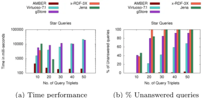
The data characteristics are summarized in Table 4. We can observe that the benchmarks have different characteristics in terms of number of vertices, number of edges, and number of distinct predicates. For instance, DBPEDIA has more diver-sity in terms of predicates (∼700) while LUBM100 contains only 13 different predicates.

The time required to build the multigraph database as well as to construct the indexes are reported in Table 5. We can note that the database building time and the corresponding size are proportional to the number of triples. Regarding

Dataset # Triples # Vertices # Edges # Edge types

DBPEDIA 33 071 359 4 983 349 14 992 982 676

YAGO 35 543 536 3 160 832 10 683 425 44

LUBM100 13 824 437 2 179 780 8 952 366 13

Table 4: Benchmark Statistics

the indexing structures, we can underline that both build-ing time and size are proportional to the number of edges. For instance, DBPEDIA has the biggest number of edges (∼15M) and, consequently, AMbER employs more time and space to build and store its data structure.

Dataset Database Index I

Building Time Size Building Time Size

DBPEDIA 307 1300 45.18 1573

YAGO 379 2400 29.1 1322

LUBM100 67 497 18.4 1057

Table 5: Offline stage: Database and Index Construction time (in seconds) and memory usage (in Mbytes)

7.2

Workload Generation

In order to test the scalability and the robustness of the dif-ferent RDF engines, we generate the query workloads con-sidering a similar setting to [7, 2, 8]. We generate the query workload from the respective RDF datasets, which are avail-able as RDF tripleset. In specific, we generate two types of query sets: a star-shaped and a complex-shaped query set; further, both query sets are generated for varying sizes (say k) ranging from 10 to 50 triplets, in steps of 10.

To generate star-shaped or complex-shaped queries of size k, we pick an initial-entity at random from the RDF data. Now to generate star queries, we check if the initial-entity is present in at least k triples in the entire benchmark, to verify if the initial-entity has k neighbours. If so, we choose those k triples at random; thus the initial entity forms the central vertex of the star structure and the rest of the en-tities form the remaining star structure, connected by the respective predicates. To generate complex-shaped queries of size k, we navigate in the neighbourhood of the initial-entity through the predicate links until we reach size k. In both query types, we inject some object literals as well as constant IRI s; rest of the IRI s (subjects or objects) are treated as variables. However, this strategy could choose some very unselective queries [7]. In order to address this issue, we set a maximum time constraint of 60 seconds for each query. If the query is not answered in time, it is not considered for the final average (similar procedure is usually employed for graph query matching [8] and RDF workload evaluation [2]). We report the average query time and, also, the percentage of unanswered queries (considering the given time constraint) to study the robustness of the approaches.

7.3

Comparison with RDF Engines

In this section we report and discuss the results obtained by the different RDF engines. For each combination of query type and benchmark we report two plots by varying the query size: the average time and the corresponding percent-age of unanswered queries for the given time constraint. We

(a) Time performance (b) % Unanswered queries

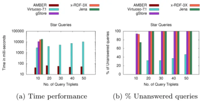
Figure 6: Evaluation of (a) time performance and (b) robustness, for Star-Shaped queries on DBPEDIA.

(a) Time performance (b) % Unanswered queries

Figure 7: Evaluation of (a) time performance and

(b) robustness, for Complex-Shaped queries on DBPEDIA.

remind that the average time per approach is computed only on the set of queries that were answered.

The experimental results for DBPEDIA are depicted in Fig-ure 6 and FigFig-ure 7. The time performance (averaged over 200 queries) for Star-Shaped queries (Fig. 6a), affirm that AMbER clearly outperforms all the competitors. Further the robustness of each approach, evaluated in terms of per-centage of unanswered queries within the stipulated time, is shown in Figure 6b. For the given time constraint, x-RDF-3X and Jena are unable to output results for size 20 and 30 onwards respectively. Although Virtuoso and gStore output results until query size 50, their time performance is still poor. However, as the query size increases, the percentage of unanswered queries for both Virtuoso and gStore keeps on increasing from ∼0% to 65% and ∼45% to 95% respectively. On the other hand AMbER answers >98% of the queries, even for queries of size 50, establishing its robustness. Analyzing the results for Complex-Shaped queries (Fig. 7), we underline that AMbER still outperforms all the competi-tors for all sizes. In Figure 7a, we observe that x-RDF-3X and Jena are the slowest engines; Virtuoso and gStore per-form better than them but nowhere close to AMbER. We further observe that x-RDF-3X and Jena are the least ro-bust as they don’t output results for size 30 onwards (Fig. 7b); on the other hand AMbER is the most robust engine as it answers >85% of the queries even for size 50. The percent-age of unanswered queries for Virtuoso and gStore increase from 0% to ∼80% and 25% to ∼70% respectively, as we increase the size from 10 to 50.

(a) Time performance (b) % Unanswered queries

Figure 8: Evaluation of (a) time performance and (b) robustness, for Star-Shaped queries on YAGO.

(a) Time performance (b) % Unanswered queries

Figure 9: Evaluation of (a) time performance and (b) robustness, for Complex-Shaped queries on YAGO.

The results for YAGO are reported in Figure 8 and Fig-ure 9. For the Star-Shaped queries (Fig. 8), we observe that AMbER outperforms all the other competitors for any size. Further, the time performance of AMbER is 1-2 or-der of magnitude better than its nearest competitor Vir-tuoso (Fig. 8a), and the performance remains stable even with increasing query size (Fig. 8b). x-RDF-3X, Jena are not able to output results for size 20 onwards. As observed for DBPEDIA, Virtuoso seems to become less robust with the increasing query size. For size 20-40, time performance of gStore seems better than Virtuoso; the reason seems to be the fewer queries that are being considered. Conversely, AMbER is able to supply answers most of the time (>98%). Coming to the results for Complex-Shaped queries (Fig. 9), we observe that AMbER is still the best in time perfor-mance; Virtuoso and gStore are the closest competitors. Only for size 10 and 20, Virtuoso seems a bit robust than AMbER. Jena, x-RDF-3X do not answer queries for size 20 onwards, as seen in Figure 9b.

The results for LUBM100 are reported in Figure 10 and Figure 11. For the Star-Shaped queries (Fig. 10), AMbER always outperforms all the other competitors for any size (Fig. 10a). Further, the time performance of AMbER is 2-3 orders of magnitude better than its closest competitor Virtuoso. Similar to the YAGO experiments, x-RDF-3X, Jena are not able to manage queries from size 20 onwards; the same trend is observed for gStore too. Further, Virtuoso always looses its robustness as the query size increases. On the other hand, AMbER answers queries for all sizes.

(a) Time performance (b) % Unanswered queries

Figure 10: Evaluation of (a) time performance and (b) robustness, for Star-Shaped queries on LUBM100.

(a) Time performance (b) % Unanswered queries

Figure 11: Evaluation of (a) time performance and (b) robustness, for Complex-Shaped queries on LUBM100.

Considering the results for Complex-Shaped queries (Fig. 11), we underline that AMbER has better time performance as seen in Figure 11a. x-RDF-3X, Jena and gStore did not sup-ply answer for size 30 onwards (Fig. 11b). Further, Virtuoso seems to be a tough competitor for AMbER in terms of ro-bustness for size 10 and 20. However, for size 30 onwards AMbER is more robust.

To summarise, we observe that Virtuoso is enough robust for Complex-Shaped smaller queries (10-20), but fails for bigger (>20) queries. x-RDF-3X fails for queries with size bigger than 10. Jena has reasonable behavior until size 20, but fails to deliver from size 30 onwards. gStore has a reasonable be-havior for size 10, but its robustness deteriorates from size 20 onwards. To summarize, AMbER clearly outperforms, in terms of time and robustness, the state-of-the-art RDF en-gines on the evaluated benchmarks and query configuration. Our proposal also scales up better then all the competitors as the size of the queries increases.

8.

CONCLUSION

In this paper, a multigraph based engine AMbER has been proposed in order to answer complex SPARQL queries over RDF data. The multigraph representation has bestowed us with two advantages: on one hand, it enables us to con-struct efficient indexing con-structures, that ameliorate the time performance of AMbER; on the other hand, the graph rep-resentation itself motivates us to exploit the valuable work done until now in the graph data management field. Thus, AMbER meticulously exploits the indexing structures to ad-dress the problem of sub-multigraph homomorphism, which

in turn yields the solutions for SPARQL queries. The pro-posed engine AMbER has been extensively tested on three well established RDF benchmarks. As a result, AMbER stands out w.r.t. the state-of-the-art RDF management sys-tems considering both the robustness regarding the percent-age of answered queries and the time performance. As a future work, we plan to extend AMbER by incorporating other SPARQL operations and, successively, study and de-velop a parallel processing version of our proposal to scale up over huge RDF data.

9.

REFERENCES

[1] G. A., M. T. ¨Ozsu, and K. Daudjee. Workload matters: Why RDF databases need a new design. PVLDB, 7(10):837–840, 2014.

[2] G. Alu¸c, O. Hartig, M. T. ¨Ozsu, and K. Daudjee. Diversified stress testing of RDF data management systems. In ISWC, pages 197–212, 2014.

[3] J. Broekstra, A. Kampman, and F. van Harmelen. Sesame: A generic architecture for storing and querying RDF and RDF schema. In ISWC, pages 54–68, 2002.

[4] E. Cabrio, J. Cojan, A. P. Aprosio, B. Magnini, A. Lavelli, and F. Gandon. Qakis: an open domain QA system based on relational patterns. In ISWC, 2012. [5] J J. Carroll, I. Dickinson, C. Dollin, D. Reynolds,

A. Seaborne, and K. Wilkinson. Jena: implementing the semantic web recommendations. In WWW, pages 74–83, 2004.

[6] O. Erling. Virtuoso, a hybrid rdbms/graph column store. IEEE Data Eng. Bull., 35(1):3–8, 2012. [7] A. Gubichev and T. Neumann. Exploiting the query

structure for efficient join ordering in sparql queries. In EDBT, pages 439–450, 2014.

[8] W.-S. Han, J. Lee, and J.-H. Lee. Turboiso: towards ultrafast and robust subgraph isomorphism search in large graph databases. In SIGMOD, pages 337–348, 2013.

[9] J. Huang, D. J Abadi, and K. Ren. Scalable sparql querying of large rdf graphs. PVLDB,

4(11):1123–1134, 2011.

[10] J. Kim, H. Shin, W.-S. Han, S. Hong, and H. Chafi. Taming subgraph isomorphism for RDF query processing. PVLDB, 8(11):1238–1249, 2015.

[11] M. Morsey, J. Lehmann, S. Auer, and A.C.N. Ngomo. Dbpedia sparql benchmark performance assessment with real queries on real data. In ISWC, pages 454–469, 2011.

[12] T. Neumann and G. Weikum. x-rdf-3x: Fast querying, high update rates, and consistency for RDF databases. PVLDB, 3(1):256–263, 2010.

[13] M. Terrovitis, S. Passas, P. Vassiliadis, and T. Sellis. A combination of trie-trees and inverted files for the indexing of set-valued attributes. In CIKM, pages 728–737. ACM, 2006.

[14] L. Zou, R. Huang, H. Wang, J. Xu Yu, W. He, and D. Zhao. Natural language question answering over RDF: a graph data driven approach. In SIGMOD Conference, pages 313–324, 2014.

[15] L. Zou, M. T. ¨Ozsu, L. Chen, X. Shen, R. Huang, and D. Zhao. gstore: a graph-based SPARQL query engine. VLDB J., 23(4):565–590, 2014.