Towards a General Solution for Detecting Traffic Differentiation At the Internet Access

(1)

HAL Id: hal-01161795

https://hal.inria.fr/hal-01161795

Submitted on 24 Jul 2015

HAL is a multi-disciplinary open access

archive for the deposit and dissemination of

sci-entific research documents, whether they are

pub-lished or not. The documents may come from

teaching and research institutions in France or

abroad, or from public or private research centers.

L’archive ouverte pluridisciplinaire HAL, est

destinée au dépôt et à la diffusion de documents

scientifiques de niveau recherche, publiés ou non,

émanant des établissements d’enseignement et de

recherche français ou étrangers, des laboratoires

publics ou privés.

Towards a General Solution for Detecting Traﬀic

Differentiation At the Internet Access

Riccardo Ravaioli, Guillaume Urvoy-Keller, Chadi Barakat

To cite this version:

Riccardo Ravaioli, Guillaume Urvoy-Keller, Chadi Barakat. Towards a General Solution for Detecting

Traﬀic Differentiation At the Internet Access. 27th International Teletraﬀic Congress (ITC-27), Sep

2015, Ghent, Belgium. �10.1109/ITC.2015.8�. �hal-01161795�

(2)

Towards a general solution for detecting traffic

differentiation at the Internet access

Riccardo Ravaioli

Universit´e Nice Sophia Antipolis Laboratoire I3S/CNRS UMR 7271

Sophia Antipolis, France

Guillaume Urvoy-Keller

Universit´e Nice Sophia Antipolis Laboratoire I3S/CNRS UMR 7271

Chadi Barakat

Inria

Abstract—In recent years network neutrality has been widely debated from both technical and economic points of view. Various cases of traffic differentiation at the Internet access have been reported throughout the last decade, in particular aimed at bandwidth consuming traffic flows. In this paper we present a novel application-agnostic method for the detection of traffic differentiation, through which we are able to correctly identify where a shaper is located with respect to the user and evaluate whether it affected delays, packet losses or both. The tool we propose, ChkDiff, replays the user’s own traffic in order to target routers at the first few hops from the user. By comparing the resulting flow delays and losses to the same router against one other, and analyzing the behaviour on the immediate router topology spawning from the user end-point, ChkDiff manages to detect instances of traffic shaping. We provide a detailed description of the design of the tool for the case of upstream traffic, the technical issues it overcomes and a validation in controlled scenarios.

I. INTRODUCTION

The neutrality of the Internet has been a hot topic ever since, around a decade ago, bandwidth-hungry applications (e.g. peer-to-peer, video, media streaming) started to gain success among users and a number of ISP’s took measures to counter possible detrimental effects on the connectivity they provided. Arbitrary decisions, as for example blocking of BitTorrent traffic in the upstream direction [1] by an operator in the US, have since then been reported. More examples include: throttling of YouTube in France [2] and Germany [3] during evening hours, when link utilization reaches its peak; degraded performance over a VPN using OpenVPN default port [4] in the US; most recently, evident decrease in performance for Netflix traffic in early 2014 by two US operators [5].

A definition for network neutrality that is generally agreed upon is that a network is neutral when all the traffic passing through it is treated equally, with no discrimination whatsoever based on the user it originates from, the destination it is intended for, its contents, the application it refers to, its relative load and time of the day. However, as described by Crowcroft [6], the Internet has never been a pure level-playing field, contrary to what neutrality proponents might affirm. Indeed, many factors can naturally contribute to a better or worse user experience, which major companies and ISP’s have often exploited: proximity to the end users with caches and replicated servers, asymmetry of inter-domain routing, NAT’s and firewalls, etc.

But since shaping is rarely revealed by official sources and certainly does not appear in Service Level Agreements (SLA’s), it becomes of utmost importance to be able to detect it from within the network. A number of tools for the detection of traffic differentiation have thus emerged in the literature in the past few years [7]–[14] (we discuss them in Section V). The method we propose here differs from existing work in its attempt to be independent both from the shaping techniques in use by ISP’s at layer 3 (IP) of the protocol stack and from the user applications that might be targeted. The idea is that a shaper whose goal is to degrade the performance of selected traffic might do so according to a variety of packet scheduling and buffer management policies, but it will typically result on the user side in larger delays and possibly more losses. Consequently, if we compare the set of delays of a flow to that of the rest of the traffic, and we proceed analogously for losses, we should be able to infer whether any shaping took place. In order for this to be valid for whatever application the user is running, we reuse her own traffic and replay it with minimal changes so that it targets the routers at the first few hops from her. If any shaper is located in proximity to one (or more) of these routers, packets going through it will have degraded performance at that hop and at all subsequent ones, thus allowing us to also pinpoint their relative position. We implemented this technique for upstream traffic in a tool we

called ChkDiff1_{, through which we can detect the presence and}

identify the location of shapers, by using the ICMP feedback provided by routers. We modify and extend here an early draft [15] of ChkDiff, in which a basic version of the tool was first described. We focus in the present work on the validation of ChkDiff, in which we stress the tool under different shaping scenarios and assess its resilience against sources of error such as traffic variation and ICMP rate limitation on routers.

The paper is organized as follows: in Section II we present the functioning of our method in details, along with a discus-sion of all the technical adjustments needed for the tool to work; in Sections III and IV we validate ChkDiff in respec-tively a controlled neutral and non-neutral environment and show that it is able to successfully detect shaping even when a large fraction of the traffic is differentiated; we compare our

1_{The code is available on a dedicated web page: riccardoravaioli.wordpress.}

(3)

method to existing work in Section V and give concluding remarks in Section VI.

II. DESIGN OF THE TOOL

The strength of ChkDiff lies on its ability to not depend on the kind of shaping technique in use by ISP’s at layer 3 of the protocol stack and on the applications (or rather, traffic flows) that might be targeted. We achieve this by implementing the following design ideas in the core of our tool:

• Use of real user traffic. We conduct all experiments with previously dumped user traffic, so that the results yielded by our tool will refer to the exact set of applications run by the user.

• Trace is left (almost) intact. This ensures that any shapers traversed by our trace will have the same behaviour they would have if the packets had been generated by their respective applications. As we will see in the following subsections, the only modifications applied to packets are in the TTL field, in order to hit the router(s) at the desired hop, and in the application payload, in which we enforce the same size on all packets so as to avoid different transmission times.

• Baseline for comparison is the entire traffic. By the definition of network neutrality, a flow that is not differentiated will be treated in the same way as the rest of the (non-differentiated) traffic, by any given router. On the other hand, a flow that is differentiated by a shaper implemented at the IP layer will typically display higher delays or losses, depending on the

scheduling and buffer management techniques in use2_{. When}

compared to the delays and losses of the rest of the trace, this flow will stand out. Our statistical analysis is based on that. We will show in the validation section that we are able to successfully detect shaping when over half of the traffic is differentiated.

The execution of ChkDiff is summarized in Algorithm 1. Algorithm 1 ChkDiff execution

1: Capture user traffic

2: for each hop h ∈ {1, 2...k} do

3: for each run r ∈ {1, 2, 3} do

4: shuffle trace

5: replay trace with T T L ← h

6: collect ICMP time-exceeded replies

7: end for

8: detect shaped flows at hop h

9: end for

10: aggregate results and locate shaper(s), if any

A traffic trace is captured during a user’s regular Internet activity; it is then processed and arranged into flows. For

2_{More specifically, a shaper will still be able to classify flows as if they}

were coming from their respective original applications, when it does so by inspecting IP, transport-layer header fields or application payloads. If it implements stateful TCP flow analysis, our replayed trace would probably bypass it. After identifying the flows to target, a shaper will apply a differentiation technique to them. ChkDiff is able to detect IP layer techniques resulting in higher delays and losses; techniques applied to higher layers, such as redirections or TCP reset injection, will not be detected.

each hop h we intend to test, we shuffle the trace so as to minimize any bias in the network conditions that our flows will experience: we keep the ordering of packets within each flow and modify the global packet ordering to be resilient to side traffic. We set the TTL field of the IP header of each packet to h and we replay the trace. Routers at hop h, if responsive, will reply with ICMP time-exceeded error messages, through which we compute single packet Round-Trip Times (RTT’s) to hop h. Any shaper located between the user and hop h must have affected packets belonging to the flows it is configured to differentiate, before the ICMP error messages were elicited. We repeat this operation 3 times for the same hop in order to filter out false positives and we claim that a flow has been shaped when it has been rejected in our statistical analysis across all three runs. Once all the first k hops have been tested, we compare the results and attempt to localize the shapers.

In the rest of this section, we will describe each of the above steps in detail.

A. Traffic trace

The first action taken by ChkDiff is to dump outgoing user traffic while the user runs her usual network applications. This is the trace that will be replayed from the end user host towards routers at the hops nearby in the following steps. Since we focus in this paper in the upstream direction, we expect the user to execute applications generating some non-trivial outgoing traffic that is not limited to HTTP requests or TCP ACK’s: for example media upload, VoIP, file sharing and instant messaging.

B. Flows and trace preparation

1) Trace classification into flows. The packets in the

dumped trace are arranged into 5-tuple flows, that is to say according to source and destination IP address, source and destination port and transport protocol.

2) Fixed-size packets. Next, we need to prepare the trace we

have to replay. Packets of different size, if sent along the same path to the same destination, will inevitably have different transmission times. As we will see in Section III, this is a non-negligible source of error if, as it is in our case, we make the assumption that the delays of all packets going along the same path should be comparable. This is especially true if we measure delays to the closest hops, where the delay variability could be low enough to be comparable to or even smaller than the difference in transmission times between small and large packets. In order to overcome this, we force every packet of our trace to be of the same size S (in Bytes), either by truncating application-level payloads larger than S Bytes, or adding random padding at the end of shorter payloads. We chose S to be 250 B, but in practice it could be any value, as long as it preserves enough of the original payload to be intercepted by shapers implementing Deep Packet Inspection (DPI), which in general looks at only the first few bytes.

3) Shuffling packets. Before replaying our trace, an

addi-tional step is required. Since our analysis will be in terms of flows, we have to ensure that they all see the same network

(4)

conditions while being injected into the network. It is therefore necessary to shuffle packets so that they exhibit such property. We assign a weight to each flow in our traffic, according to its original size in packets and normalized by the sum of all flows sizes, such that all weights sum to 1. For a trace with f flows,

any flow i with size si, in number of packets, will have weight

pi = si/P

f

k=1sk. A queue is thus created for each flow,

where the per-flow packet order is maintained, since it might reveal useful information to a shaper for flow identification. We now pick packets randomly from each queue according to the flow weight and put them aside, ready to be replayed. Whenever a queue becomes empty, its weight is set to 0 and weights of all other flows are updated accordingly, so that they always sum to 1. By popping packets from each queue in the above fashion, we obtain for every flow an ordered sequence of 0’s and 1’s indicating whether a packet in the resulting shuffled trace came from that flow or not. Given a flow i, such sequence of 0s and 1s can be seen as a Bernoulli process with a probability equal to the weight of flow i, let us

say pi. Now, if we consider the spacing (or inter-packet time)

Wibetween any two consecutive packets from flow i, we can

see that it follows a geometric distribution with parameter pi:

P (Wi= w) = (1−pi)w−1pi. The geometric distribution being

the discrete version of an exponential distribution, packets of flow i see the real network conditions according to the PASTA property (Poisson Arrivals See Time Averages) [16]. As this property applies to all flows, it enables us to reach our initial goal: letting all flows observe the same network conditions, provided that the network offers a stationary service.

Furthermore, shuffling is particularly useful when having to counteract side traffic and ICMP rate limitation, as we will see shortly.

C. Replay

1) ICMP rate limitation. In a previous work [17], we

studied the responsiveness of routers to TTL-limited probes. Through a large measurement campaign, we examined pos-sible bias in the Round-Trip Times of these probes and how ICMP rate-limitation is implemented on routers. We demon-strated that there did not appear to be any correlation between a slow or high probing rate (in the range [1, 4000] packets per second) and the resulting Round-Trip Times. In other words, even at high rates, we were not hitting any capacity limits that might have slowed down the generation of ICMP messages and contributed to the total packet delay. This is good news, since it tells us that the choice of probing rate does not mar the delays we obtain. There will definitely be a delay component due to the generation of the ICMP error message (estimated to be in the order of the submillisecond [18]), since it takes place in the router slow path, which is usually implemented in software instead of hardware and does not have high priority compared to other router operations. But this delay component will have roughly the same weight in all RTTs toward the same router and therefore will not constitute a source of error.

When using TTL-limited probes as in our case, we must also make sure that we obtain a sufficient number of replies,

since it is a fairly widespread practice for manufacturers and network administrators to limit at a fixed maximum rate the re-sponsiveness of routers to these expiring probes. We tested 850 routers from PlanetLab hosts up to hop 5 and demonstrated that ICMP rate limitation is implemented as an on-off process with typical values in [20, 500] packets per second (pps). In light of this, the shuffling technique presented above has the undoubted advantage that unanswered probes would be spread fairly evenly across flows, since flow packets themselves are spread evenly across the trace. A non-shuffled trace replayed to an ICMP rate-limiting router would instead incur more variable losses among flows, which would inevitably impair any loss analysis. We will discuss the robustness of our tool to ICMP rate limitation in Section IV.

2) Testing the first k hops. In order to locate the position

of a shaper, we need to replay the shuffled trace as many times as the number of hops we want to test, by increasing the IP TTL of all packets at every experiment. For the choice of k, a value of 3 or 4 should suit most cases and provide a large enough picture of what happens at the user’s Internet access, including ISP routers and those right after the ISP boundaries. The user trace being made of flows with different IP destination addresses, testing routers that are further away is of increasing complexity due to a reduction in terms of samples per router as we move away from the user.

D. Results analysis

We focus our analysis on the study of Round-Trip Times and losses. In both cases, the approach is similar: we consider large flows only, that is those with at least 20 answered packets (a typical minimum sample size in statistical analysis), and we analyze these flows one at a time, comparing them against all the rest of the traffic as a whole (large and small flows indifferently).

1) Delays. We compare the distribution of delays of a

flow to the delay distribution of the rest of the trace using a statistical test. Our null hypothesis is that, in an envi-ronment without differentiation, if we sample the total set of delays obtained, they will all appear to be drawn from the same distribution as all the other delays of the trace. We conduct our analysis by applying two-sample one-sided Kolmogorov-Smirnov test, which has the benefit of being non-parametric, in that it does not make assumptions on the underlying distribution of the data it is checking. The test takes as statistic the maximum vertical deviation between the Cumulative Distribution Functions (CDF’s) of two samples. We chose the one-sided version of this test because, while the two-sided Kolmogorov-Smirnov test looks for the maximum vertical deviation between two curves without including in its result whether this vertical distance was due to the first curve being above the second one or the other way around, the one-sided version looks for this deviation in one given direction. Applied to our scenario, we can test whether a flow experienced worse (i.e. larger) delays than the rest of the trace by checking whether its CDF lies below the CDF of its baseline, and to which extent.

(5)

Fig. 1: An example with shapers at different hops.

hop 1 hop 2 hop 3 hop 4 shapers? flow 0 D 6 6 6 hop 2 flow 1 D D D 6 hop 4 flow 2 D D unresp D none flow 3 D D unresp 6 hops 3,4 flow 4 D D unresp unresp not until hop 2

Fig. 2: ChkDiff expected output.

2) Losses. In order to check if the loss rate of a flow differs

significantly from that of the rest of the trace, we proceed by using an argument inspired from the binomial distribution. If we want to examine the losses (i.e. the number of unanswered packets) experienced by flow i, we let p be the loss rate of the

rest of the traffic as a whole, and si be the original number

of packets of flow i. If the loss events of flow i were not

caused by a shaper, its number of losses li can be modeled

as a binomial random variable of parameters B(si, p). To test

whether this holds true, we can approximate this binomial as a

normal random variable of parameters N (sip, sip(1 − p)) and

verify that the loss events lilie within α standard deviations of

the normal mean. With α being a function of the significance

level we want to achieve, we check that ps−αpp(1 − p)si<

li< psi+ αpp(1 − p)si. The right side of this last condition

is the one we are interested in, as it indicates that the flow experienced more losses than it should have, and it is what we check in our analysis.

3) Repetition of experiments. Statistical tests are operated

at a certain confidence level, which in our tool we set to 99%. Due to the high number of flows in a user trace, we are bound to have a number of false positives, whatever action we take. To work around this issue, we adopt a simple strategy. We repeat an experiment three times (at the same constant probing rate) to router(s) at the same hop-distance and claim that a flow has been shaped only when it was rejected in all three runs. E. Results Aggregation

After collecting traces and analyzing delays and losses for the first k hops, we need aggregate results in order to attempt to localize the shaper, if ever a flow was rejected in any of those hops. A shaper positioned right before hop h, with h ∈ {1, 2, ... k}, will cause targeted flows to fail the delay or loss analysis (or both) on all hops ≥ h. When ChkDiff detects this, it declares the flow as being shaped on the hop-segment between h and the previous responsive router. We show an example with routers up to hop 4 in Figure 1. We assume that there is a number of non-differentiated flows from the user trace passing through each router besides the four shown in the figure, and that they contribute to the baseline for the statistical analysis. In Figure 2 we provide the expected output from ChkDiff based on this scenario. A shaper for flow 0 is deployed right before the router at hop 2: this means that flow

0 will pass the analysis at hop 1, but will not at all successive hops. Flow 1 is a similar case, but at the edge of the tested hops. At hop 3 an unresponsive router, that is to say a router that was configured not to reply to expiring packets, generates a gap in our assessment, which might be compensated by the results at the next hop. If at the next hop a flow (flow 2) continues to pass the test, we can safely claim that it was not shaped along the whole path under consideration. If instead the flow fails the test, as we showed for flow 3 in our example, we can only say that at hop 3 and 4 it encountered a shaper, without being more specific. Finally, if the next hop is also unresponsive, for a flow like flow 4, our conclusion is simply that no shapers were detected up to the last hop where the flow passed the analysis.

III. VALIDATION IN A NEUTRAL SCENARIO

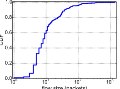
Before validating ChkDiff in the presence of traffic differen-tiation, it is important to justify some measures we take when replaying a user trace: forcing the same size in all packets and aggregating results across 3 experiments. The packet trace we used here and in Section IV was captured in a time-window of 3 minutes of a typical Internet session, in which we performed picture uploading on a social network, browsing on a news site, and sent a few chat messages. The trace is made of 6733 packets, arranged into 275 flows, of which 61 are large (i.e. they have more than 20 packets) and comprise 76.8% of the total amount of packets. The exact distribution of flow sizes is shown in Figure 3.

We claimed in Section II-B2 that, by fixing the packet size

100 ₁₀1 ₁₀2 ₁₀3 flow size (packets)

0.0 0.2 0.4 0.6 0.8 1.0 CDF

Fig. 3: Distribution of flow sizes, in number of packets, for the packet trace used for validation.

(6)

0 1 2 3 4 5

no. of false positives

0.0 0.2 0.4 0.6 0.8 1.0 CDF KS original fixed size

Fig. 4: Incidence of false positives when the replayed trace contains unaltered original packets, and when it contains packets of the same size. Results are over 1 run.

to a constant value for all packets in a trace, we were able to remove a considerable fraction of errors in the delay analysis. We now show the incidence of false positives when packets are the original size and when they are padded or truncated to a constant value. For each of the two options, we ran ChkDiff 100 times in a controlled setup with no differentiation towards a router under our control at hop 2. In Figure 4 we compare the CDFs of the number of false positives for each experiment. The improvement is evident: we remove all errors in 70% of experiments and are left with 30% of experiments showing mostly 1 false positive. The next step is to aggregate the results of multiple runs, as described in Section II-D3 and see if these errors disappear. We ran ChkDiff 100 times and observed indeed that no false positives emerged when considering just two runs. In order to have a safe margin of error, we use by default three runs in ChkDiff.

IV. VALIDATION IN A NON-NEUTRAL SCENARIO

We tested how the tool copes with different shaping and network settings in a controlled experimental setup. We fo-cused on two scenarios: Scenario 1, in which we throttle the bandwidth of selected flows, and Scenario 2, where we apply uniform packet drops. In our setup, a user machine is connected through cable to a middle box, which operates both as a gateway and a shaper, and which is, in turn, connected to a Cisco router under our control, where our probes expire. In the middle box, we deployed a shaper with Dummynet [19], a popular and versatile network emulation tool. The configuration we used is depicted in Figure 5: incoming packets are directed to either the upper or lower pipe on the left side, depending on whether they belong respectively to the flows to shape or not. The upper pipe is traversed by all flows that we intend to shape; in Scenario 1 it has its own bandwidth bw and queue size, and in Scenario 2 it induces uniform losses at rate lr. The lower pipe compensates for the transmission delay produced by the upper pipe in Scenario 1: it adds this constant delay component to the packets of all non-differentiated flows, so that only the queueing delay in the upper pipe constitutes the discriminating factor between shaped and non-shaped packets. In scenario 2, it produces no effect. Finally, all packets meet at the pipe on the right-hand

shaping pipe

compensating pipe

100 Mbit/s pipe

Fig. 5: Middle-box configuration.

side, which emulates a 100 Mbit/s link. In Scenario 2 this

pipe induces a uniform loss rate lrall to all flows. All pipes

are configured with a buffer size of 100 packets and a droptail buffer management policy.

A. One shaped flow

We start by examining a scenario in which only one flow is being differentiated by the shaper. We proceeded by taking the trace previously described and adding an extra flow of which we varied the number of packets in order for it to be a fraction f r of the total amount of packets of the trace. This is the flow that will be targeted by the shaper. Our results are in terms of precision and recall, which show respectively the fraction of detected flows that we know are indeed shaped, and the

fraction of shaped flows that are correctly detected3. Perfect

performance translates into a precision and recall of 100%.

1) Shaping pipe (Scenario 1). In this configuration the

bandwidth bw of the upper pipe on the left side is set as a function of the average sending rate r (in bits per second) of the shaped flow, computed before the experiment begins.

We chose bw = kbwr, so that a fraction kbw ∈ (0, 1]

of packets of the shaped flow would use all the available pipe bandwidth bw and the rest would queue up. We ran

ChkDiff 3 times for each combination of kbw and f r, with

kbw ∈ {0.2, 0.4, 0.6, 0.8, 1.0} and f r ∈ {0.2, 0.4, 0.6, 0.8}.

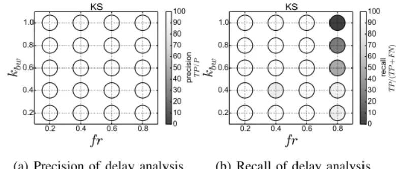
The results are shown in Figure 6, where the colour of each circle reflects the percentage of precision or recall obtained. In this basic scenario, we see that the delay test manages to

always identify the shaped flow. At kbw = 1 we observe that

the flow still experienced some queueing, as a result of the pipe bandwidth being a function of the average sending rate of the flow and not of its instantaneous rate.

2) Uniform drops (Scenario 2). Our goal in Scenario 2

is to verify to which extent ChkDiff manages to identify a shaped flow, when losses affect a selected flow and the entire traffic at different rates. We configured the shaper so that the upper pipe in Figure 5 drops a fraction lr of the packets of the flow to shape, and the pipe on the right-hand

side, where all traffic goes, has a drop rate of lrall. We

varied again the size of the targeted flow and ran experiments with f r ∈ {0.2, 0.4, 0.6, 0.8}. For reasons of space, we do not include the graphs on precision, since all results show

3_{We define precision as being the number of true positives (TP) over the}

number of positives (P), and recall as the number of true positives over the sum of true positives and false negatives (FN), that is to say over the number of flows that we know were shaped. For more details, refer to http://en.wikipedia. org/wiki/Precision and recall

(7)

0.2 0.4 0.6 0.8

fr

0.2 0.4 0.6 0.8 1.0

k

bw KS 0 10 20 30 40 50 60 70 80 90 100 precision TP /P

(a) Precision of delay analysis

0.2 0.4 0.6 0.8

fr

0.2 0.4 0.6 0.8 1.0

k

bw KS 0 10 20 30 40 50 60 70 80 90 100 recall TP / ( TP + FN )

(b) Recall of delay analysis

Fig. 6:Precision and recall of the delay analysis, for the case of one

shaped flow in Scenario 1.

0.0 0.2 0.4 0.6 0.8

lr

all 0.0 0.2 0.4 0.6 0.8 1.0

lr

sh ap ed Loss test (fr=20%) 0 10 20 30 40 50 60 70 80 90 100 recall TP / ( TP + FN )

(a) Recall when f r = 20%

0.0 0.2 0.4 0.6 0.8

lr

all 0.0 0.2 0.4 0.6 0.8 1.0

lr

sh ap ed Loss test (fr=40%) 0 10 20 30 40 50 60 70 80 90 100 recall TP / ( TP + FN ) (b) Recall when f r = 40% 0.0 0.2 0.4 0.6 0.8

lr

all 0.0 0.2 0.4 0.6 0.8 1.0

lr

sh ap ed Loss test (fr=60%) 0 10 20 30 40 50 60 70 80 90 100 recall TP / ( TP + FN ) (c) Recall when f r = 60% 0.0 0.2 0.4 0.6 0.8

lr

all 0.0 0.2 0.4 0.6 0.8 1.0

lr

sh ap ed Loss test (fr=80%) 0 10 20 30 40 50 60 70 80 90 100 recall TP / ( TP + FN ) (d) Recall when f r = 80%

Fig. 7:Recall of loss analysis as we vary f r, for the case of uniform

drops on the whole traffic and on one selected flow (Scenario 2).

a precision of 100%, that is to say we never encountered any false positives or, in other words, all the flows detected by ChkDiff as being shaped were indeed shaped. On the other hand, some false negatives (i.e. shaped flows that go undetected) did occur, so our analysis will focus on recall. In Figure 7 we present the results for this scenario. On the

X-axis we plot the loss rate lrall for all packets of the trace,

whereas on the Y-axis we show the overall loss-rate lrshaped

experienced by the shaped flow: 1 − (1 − lr)(1 − lrshaped).

The tool achieves 100% recall in all cases except those in which, with a low f r and a fairly high (≥ 40%) overall loss rate, the loss rate of the shaped flow is close to the global one. The added loss rates on the lower diagonal of the graphs correspond to lr = 0.05, which could be too low to be noticeable on samples of relatively small size. In all other cases, the tool correctly identified the shaped flow.

0.2 0.4 0.6 0.8

fr

0.2 0.4 0.6 0.8 1.0

k

bw KS 0 10 20 30 40 50 60 70 80 90 100 precision TP /P

(a) Precision of delay analysis

0.2 0.4 0.6 0.8

fr

0.2 0.4 0.6 0.8 1.0

k

bw KS 0 10 20 30 40 50 60 70 80 90 100 recall TP / ( TP + FN )

(b) Recall of delay analysis

Fig. 8: Precision and recall of the delay analysis, for the case of

multipleshaped flows, in Scenario 1.

0.0 0.2 0.4 0.6 0.8

lr

all 0.0 0.2 0.4 0.6 0.8 1.0

lr

sh ap ed Loss test (fr=20%) 0 10 20 30 40 50 60 70 80 90 100 recall TP / ( TP + FN )

(a) Recall when f r = 20%

0.0 0.2 0.4 0.6 0.8

lr

all 0.0 0.2 0.4 0.6 0.8 1.0

lr

sh ap ed Loss test (fr=40%) 0 10 20 30 40 50 60 70 80 90 100 recall TP / ( TP + FN ) (b) Recall when f r = 40% 0.0 0.2 0.4 0.6 0.8

lr

all 0.0 0.2 0.4 0.6 0.8 1.0

lr

sh ap ed Loss test (fr=60%) 0 10 20 30 40 50 60 70 80 90 100 recall TP / ( TP + FN ) (c) Recall when f r = 60% 0.0 0.2 0.4 0.6 0.8

lr

all 0.0 0.2 0.4 0.6 0.8

lr

sh ap ed Loss test (fr=80%) 0 10 20 30 40 50 60 70 80 90 100 recall TP / ( TP + FN ) (d) Recall when f r = 80%

Fig. 9:Recall of loss analysis as we vary f r, for the case of uniform

drops on the whole traffic and on multiple selected flows (Scenario 2).

B. Multiple shaped flows

We now move to a more complex scenario, in which multiple flows are being targeted by the shaper. In order to select which flows to shape, given a fraction f r of the trace size to differentiate, we iteratively picked the flow whose size (in Bytes) was the closest to the target f r, until the total amount was reached.

1) Shaping pipe (Scenario 1). We set the bandwidth bw

of the shaping pipe as a function of the average sending rate of all packets belonging to the flows to shape. All shaped flows pass through the same shaping pipe so as to be able to compensate for one transmission time only in the lower pipe. We present the results for this scenario in Figure 8. While the precision reached appears to be optimal, the recall plots show that, quite expectedly, when the shaped flows amount to a large fraction of the trace, the baseline for comparison

(8)

becomes too weakened for the test to work.

2) Uniform drops (Scenario 2). In the scenario with

uni-form drops, we used a different shaping pipe for each flow to differentiate, in order to have the same loss rate lr for all shaped flows. Results are provided in Figure 9, where we omitted the plots on precision for the same reason mentioned before. In the four subplots, we are mostly interested in the

area with lrall ∈ [0.0, 0.2], as it best represents a realistic

setting: in a network with no (0%) or relatively high (20%) packet drops, a shaper causes losses of various degrees to part of the traffic passing through it. For completeness, we also show cases with higher losses and a large fraction of affected traffic. When 20% of the traffic is targeted, we are able to detect all differentiated flows, except when the shaped flows experience just 5% more of losses, on top of the 20% overall loss rate of the trace. We observe that, as we shape an increasing fraction of the trace, the loss analysis significantly degrades. The reason is that, with several flows being differentiated, the baseline will necessarily include more and more shaped flows and the statistical analysis will be impacted. However, this constitutes an extreme case for our tool and it is unlikely to be encountered in practice.

C. ICMP rate limitation

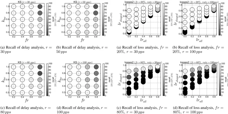
Lastly, we wanted to verify how resilient our analysis is when we encounter a router that implements ICMP rate limitation. We tested ChkDiff in the same experimental setups as before and configured the router to respond at most at 20 pps (with a burst size of 20 packets and a period of 1 second), a common setting we found for Cisco routers [17]. We repeated the experiments of Scenarios 1 and 2 at different sending rates (30, 50, 80 and 100 pps) higher than the ICMP rate limitation threshold. Our aim is to stress our tool when an additional source of losses is present and see how high our sending rate r can be, with respect to the rate limitation implemented on the router side, while still minimizing errors. In Figure 10 we show the recall plots of the delay analysis in the case of Scenario 1, where a shaping pipe throttles the bandwidth of multiple selected flows. Since ICMP rate limitation only causes packet drops, it is no surprise that the delays are no more affected than they were in the previous case when the router was fully responsive (Figure 8b). We omit here and in the next scenario the results for one shaped flow, since they always showed maximum precision and recall. We conducted again the experiments of Scenario 2, where uniform drops are applied to selected flows and to the whole traffic with different probabilities, and we provide the results in Figure 11. For constraints of space, we only show cases with f r ∈ {0.2, 0.8} and r ∈ {30, 100} pps, i.e. the extreme values considered in the previous scenario. We observe that the loss test experiences considerable degradation only in the extreme case of multiple shaped flows corresponding to 80% of the trace. Varying the probing rate from 1.5 (30 pps, with a router-induced loss rate of 33%) to 5 times (100 pps, with a router-induced loss rate of 80%) the ICMP rate limitation

threshold of the router does not appear to alter significantly the results.

D. A more complex scenario

In a realistic setting, if a user dumps her own traffic while some TCP flows are being targeted by a shaper that throttles their bandwidth, the sending rate of these flows inside the captured trace will already have been reduced by the shaper. If ChkDiff replays this trace at its original sending rate, the TCP flows that were previously throttled will now comply with the shaper’s policies and will not of course experience any further degradation. It is therefore important to scale up our probing rate with respect to the original one, in order to be able to trigger and detect the presence of a shaper.

We set up a scenario with a shaper, ICMP rate limitation and side traffic. In the same way as in Section IV-A, we created a flow constituting 20% of the total trace size and injected it in our trace so that it would be evenly spread out

and have consequently a constant sending rate rf low. The

shaper was configured as in the previous case of a shaping pipe affecting one flow only, and its bandwidth was set to rf low. The router activated ICMP rate limitation at 50 pps,

a common value for Juniper routers [17]. Finally, we added some cross traffic flowing on average at 20% of our sending rate and implemented it as a series of bursts of ping packets following a Poisson process. We configured the bandwidth of the pipe on the right-hand side in Figure 5 to be equal to the sum of the rate of the trace and of the cross traffic. This way, the whole trace also experiences queueing.

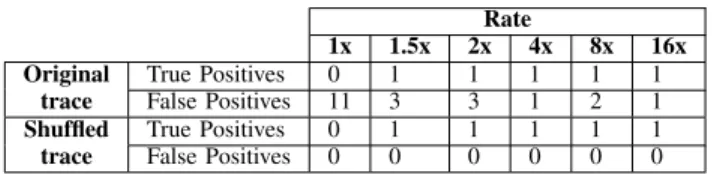
In this setup, we assess whether a shuffled trace replayed at a constant rate is indeed more robust to transient network con-ditions than the original trace replayed as it is. We increased the probing rate r by a factor of 1.5, 2, 4, 8 and 16 times the

original probing rate rorig of the trace (with rorig = 64 pps)

and counted in Table I the number of false positives of the delay analysis across 3 runs. We see that, even though in both cases we correctly identify the shaped flow already at 1.5x, we never encounter any false positives when replaying a shuffled trace. With the original trace, on the other hand, we always obtained some false positives; their number seems to decrease with high probing rates only because the amount of flows with sufficient samples also decreases.

V. RELATEDWORK

A number of tools for the detection of traffic differentiation have been proposed in the literature in the past few years.

Rate 1x 1.5x 2x 4x 8x 16x Original trace True Positives 0 1 1 1 1 1 False Positives 11 3 3 1 2 1 Shuffled trace True Positives 0 1 1 1 1 1 False Positives 0 0 0 0 0 0

TABLE I: Number of true and false positives when replaying the original and a shuffled trace at different sending rates.

(9)

0.2 0.4 0.6 0.8

fr

0.2 0.4 0.6 0.8 1.0

k

bw KS (r=30pps) 0 10 20 30 40 50 60 70 80 90 100 recall TP / ( TP + FN )

(a) Recall of delay analysis, r = 30 pps 0.2 0.4 0.6 0.8

fr

0.2 0.4 0.6 0.8 1.0

k

(b) Recall of delay analysis, r = 50 pps 0.2 0.4 0.6 0.8

fr

0.2 0.4 0.6 0.8 1.0

k

(c) Recall of delay analysis, r = 80 pps 0.2 0.4 0.6 0.8

fr

0.2 0.4 0.6 0.8 1.0

k

(d) Recall of delay analysis, r = 100 pps

Fig. 10: Scenario 1 with multiple shaped flows and ICMP rate

limitation at 20 pps. 0.0 0.2 0.4 0.6 0.8

lr

all 0.0 0.2 0.4 0.6 0.8 1.0

lr

sh ap ed losses2 (fr=20%, rate=30pps) 0 10 20 30 40 50 60 70 80 90 100 recall TP / ( TP + FN )

(a) Recall of loss analysis, f r = 20%, r = 30 pps 0.0 0.2 0.4 0.6 0.8

lr

all 0.0 0.2 0.4 0.6 0.8 1.0

lr

(b) Recall of loss analysis, f r = 20%, r = 100 pps 0.0 0.2 0.4 0.6 0.8

lr

all 0.0 0.2 0.4 0.6 0.8 1.0

lr

(c) Recall of loss analysis, f r = 80%, r = 30 pps 0.0 0.2 0.4 0.6 0.8

lr

all 0.0 0.2 0.4 0.6 0.8 1.0

lr

(d) Recall of loss analysis, f r = 80%, r = 100 pps

Fig. 11: Scenario 2 with multiple shaped flows and ICMP rate

limitation at 20 pps.

A work that has some aspects in common with ChkDiff is NetPolice [7], where the authors were able to detect differ-entiation in backbone networks with the use of TTL-limited probes. Using synthetic traces made of HTTP, peer-to-peer, BitTorrent and other application flows, they probed ingress and egress routers of backbone ISP’s from a large set of PlanetLab nodes in order to notice any difference in loss rates along the same path segment: if any difference was observed, they tried to attribute it to content-based differentiation (with the HTTP flow as baseline) or, when the discrepancy was between different IP sources or destinations, to routing-based differen-tiation. Our approach does leverage TTL-limited probes, but it is client-oriented (in a traceroute-like manner), it focuses on a user’s access ISP, and does not make assumptions on which flows should be considered as non-differentiated in its analysis.

One of the first tools presented to the scientific community was BT-test [8], which checks for TCP reset packets injected by ISP’s during the replaying of a typical BitTorrent packet exchange between a user and controlled server. Its aim was to disclose a practice that had been recently reported by some US-based users. The same authors later proposed a more comprehensive tool, Glasnost [9], that compares the maximum throughput of an application flow (e.g. BitTorrent, YouTube, etc) to that of a control flow whose packets are the same as in the application flow except for their payload, which is randomized. The packets of the two flows are interleaved so as to experience the same network conditions and are replayed to a server. This technique expects traffic differentiation to

happen at the application layer, by means of deep packet inspection, and to result in lower throughput for the affected application. ChkDiff is also able to detect such cases, since a lower throughput is the result of higher packet delays, but we don’t make the assumption that a shaper targets a specific application and that it discriminates according to packet payloads.

A tool that also focuses on a specific application and control flow is DiffProbe [10], which attentively analyses the delay and loss distributions of the two flows during a replaying phase at the normal application sending rate and a replaying phase at a higher rate, which attempts to create congestion at possible shapers along the path. The control flow is crafted much in the same way as previously described, with the addition of transport layer fields such as port number being modified in order to bypass shapers. This tool was soon followed by ShaperProbe [11], which assumes that differentiation happens through a token bucket and tries to infer its parameters (buffer size and processing rate). It sends trains of packets back-to-back to a server and, if they traverse a shaper, it expects to observe a level shift in the received rate at the destination. While both methods undoubtedly provide more insight than ChkDiff on the characteristics of shapers, they analyze the behaviour of one application at a time and, even if in principle they can adapt to any application, they are in practice limited to the packet traces provided with the executables (i.e. Skype, in this case). Packsen [13] has a similar approach to DiffProbe, but it improves on it by using a less computationally expensive statistical analysis in order to infer the shaper type and

(10)

parameters.

The only work so far described in literature to use passive measurements is Nano [12]. It passively monitors various per-formance metrics on the existing traffic of a user and compares them to those of other users whose results were collected at roughly the same time of the day, with similar machine setup and geographical position, but who were connected to a different ISP. With all confounding factors being equal, causal inference between degraded performance and (alleged) ISP shaping can be established. This tool has two great advantages: it is truly application and shaping technique agnostic. Its main drawback is that, in order for it work, it requires a substantial number of users for all values of the different confounding factors mentioned above.

More recently, a theoretical framework for the inference and localization of neutrality violating links has been pro-posed [14]. After conducting measurements from different vantage points traversing the same links, it builds a linear system of equations in the same fashion as in network perfor-mance tomography. When the network is neutral, such system is supposed to be solvable and it infers properties of the links. When instead a link is not neutral, the measurements are inconsistent and the system unsolvable. The deployment of such method would require a large and diverse user base, where several vantage points perform measurements on the same set of paths and send the results to a central server, which would process the data and infer differentiation. Our approach is instead confined to the network performance experienced by the end user who runs the tool: no aggregation of results across users is necessary.

VI. CONCLUSION

In this paper we presented ChkDiff, a novel tool for the detection of traffic differentiation at the Internet access. After replaying the user outgoing traffic to the routers at the first few hops, it applies a statistical test to delays and losses in order to infer whether any of the replayed flows experienced degraded performance. We validated ChkDiff in a controlled environment with different setups and showed its robustness to ICMP rate limitation.

In the future, we intend to extend ChkDiff so that it includes a test for downstream traffic, which will be shuffled, spoofed and replayed to the user from a server. We also need to encompass in our method those cases of neutrality violations that do not result in larger delays or losses, such as TCP reset injection. Finally, we plan to test ChkDiff in the wild and run it from different vantage points, in order to map the behaviour of different ISP’s.

ACKNOWLEDGMENTS

This work was funded by the French Government (National Research Agency, ANR) through the ”Investments for the Future” Program reference #ANR-11-LABX-0031-01.

REFERENCES

[1] “Dslreports: comcast is using sandvine to manage p2p connections.” [Online]. Available: http://www.dslreports.com/forum/r18323368-Com%20cast-is-using-Sandvine-to-manage-P2P-Connections. [2] “Respect my net.” [Online]. Available: http://respectmynet.eu/view/205 [3] “Respect my net.” [Online]. Available: http://respectmynet.eu/view/196 [4] “I just doubled my pia vpn throughput that i am getting on my router by switching from udp:1194 to tcp:443,” 2014. [Online]. Available: http://www.reddit.com/r/VPN/comments/1xkbca/i just doubled my pia vpn throughput that i am

[5] “Netflix performance on verizon and comcast has been dropping for months,” 2013. [Online]. Avail-able: http://arstechnica.com/information-technology/2014/02/netflix-performance-on-verizon-and-comcast-has-been-dropping-for-months [6] J. Crowcroft, “Net neutrality: the technical side of the debate: a white

paper,” SIGCOMM Comput. Commun. Rev., vol. 37, pp. 49–56, January 2007. [Online]. Available: http://doi.acm.org/10.1145/1198255.1198263 [7] Y. Zhang, Z. M. Mao, and M. Zhang, “Detecting traffic differentiation in backbone isps with netpolice,” in In Proceedings of the Internet Measurement Conference (IMC, 2009.

[8] M. Dischinger, A. Mislove, A. Haeberlen, and K. P. Gummadi, “De-tecting bittorrent blocking,” in Proceedings of the 8th ACM SIGCOMM Conference on Internet Measurement (IMC’08), Vouliagmeni, Greece, October 2008.

[9] M. Dischinger, M. Marcon, S. Guha, K. Gummadi, R. Mahajan, and S. Saroiu, “Glasnost: Enabling end users to detect traffic differentiation,” in Proceedings of the 7th Symposium on Networked Systems Design and Implementation (NSDI), San Jose, CA, Apr 2010.

[10] P. Kanuparthy and C. Dovrolis, “Diffprobe: detecting isp service dis-crimination,” in Proceedings of the 29th conference on Information communications, ser. INFOCOM’10. Piscataway, NJ, USA: IEEE Press, 2010, pp. 1649–1657.

[11] ——, “Shaperprobe: end-to-end detection of isp traffic shaping using active methods,” in Proceedings of the 2011 ACM SIGCOMM conference on Internet measurement conference, ser. IMC ’11. New York, NY, USA: ACM, 2011, pp. 473–482.

[12] M. B. Tariq, M. Motiwala, N. Feamster, and M. Ammar, “Detecting network neutrality violations with causal inference,” ACM SIGCOMM CoNext, p. 289, 2009.

[13] U. Weinsberg, A. Soule, and L. Massouli´e, “Inferring traffic shaping and policy parameters using end host measurements,” in INFOCOM, 2011, pp. 151–155.

[14] Z. Zhang, O. Mara, and K. Argyraki, “Network neutrality inference,” in Proceedings of the 2014 ACM Conference on SIGCOMM, ser. SIGCOMM ’14. New York, NY, USA: ACM, 2014, pp. 63–74. [15] R. Ravaioli, C. Barakat, and G. Urvoy-Keller, “Chkdiff: checking traffic

differentiation at internet access,” in Proceedings of the 2012 ACM conference on CoNEXT student workshop. ACM, 2012, pp. 57–58. [16] R. W. Wolff, “Poisson arrivals see time averages,” Operations Research,

vol. 30, no. 2, pp. 223–231, 1982.

[17] R. Ravaioli, G. Urvoy-Keller, and C. Barakat, “Characterizing icmp rate limitation on routers,” in IEEE International Conference on Communi-cations (ICC), 2015.

[18] R. Govindan and V. Paxson, “Estimating router icmp generation delays,” in Passive & Active Measurement (PAM), 2002.

[19] M. Carbone and L. Rizzo, “Dummynet revisited,” SIGCOMM Comput. Commun. Rev., vol. 40, no. 2, pp. 12–20, Apr. 2010.