HAL Id: hal-00707543
https://hal.archives-ouvertes.fr/hal-00707543
Submitted on 13 Jun 2012
HAL is a multi-disciplinary open access
archive for the deposit and dissemination of
sci-entific research documents, whether they are
pub-lished or not. The documents may come from
teaching and research institutions in France or
abroad, or from public or private research centers.
L’archive ouverte pluridisciplinaire HAL, est
destinée au dépôt et à la diffusion de documents
scientifiques de niveau recherche, publiés ou non,
émanant des établissements d’enseignement et de
recherche français ou étrangers, des laboratoires
publics ou privés.
Using Constraint Programming to Verify DOPLER
Variability Models
Raúl Mazo, Paul Grünbacher, Wolfgang Heider, Rick Rabiser, Camille
Salinesi, Daniel Diaz
To cite this version:
Raúl Mazo, Paul Grünbacher, Wolfgang Heider, Rick Rabiser, Camille Salinesi, et al.. Using
Con-straint Programming to Verify DOPLER Variability Models. 5th International Workshop on
Variabil-ity Modelling of Software-intensive Systems (VaMos’11), Jan 2011, Namur, Belgium. �hal-00707543�
Using Constraint Programming to Verify DOPLER
Variability Models
Raul Mazo
1,4,
Paul Grünbacher
2,3,
Wolfgang Heider
3,
Rick Rabiser
3,
Camille Salinesi
1,
Daniel Diaz
11
CRI, Panthéon Sorbonne University, Paris, France
2Institute for Systems Engineering and Automation, Johannes Kepler University, Linz, Austria
3Christian Doppler Laboratory for Automated Software Engineering, Johannes Kepler University, Linz, Austria
4Ingeniería de Sistemas, University of Antioquia, Medellín, Colombia
[email protected], [email protected], {heider, rabiser}@ase.jku.at,
{camille.salinesi, daniel.diaz}@univ-paris1.fr
ABSTRACT
Software product lines are typically developed using model-based approaches. Models are used to guide and automate key activities such as the derivation of products. The verification of product line models is thus essential to ensure the consistency of the derived products. While many authors have proposed approaches for verifying feature models there is so far no such approach for decision models. We discuss challenges of analyzing and verifying decision-oriented DOPLER variability models. The manual verification of these models is an error-prone, tedious, and sometimes infeasible task. We present a preliminary approach that converts DOPLER variability models into constraint programs to support their verification. We assess the feasibility of our approach by identifying defects in two existing variability models.
Categories and Subject Descriptors
D.2.1 [Requirements/Specifications]: Languages. D.2.4 [Software/Program Verification]: Formal methods.
General Terms
Algorithms, Experimentation, Languages, Verification.
Keywords
Verification, Decision-oriented variability models, software product lines, constraint programming.
1. INTRODUCTION AND MOTIVATION
Models are used in software product lines to define, analyze, and communicate the variability of systems and to support the derivation of new products. For instance, feature-oriented modeling languages [5, 12], decision-oriented approaches [4, 18], UML-based techniques [10], and orthogonal approaches [16] have been proposed for defining variability. The formal verification of variability models is an important issue in product line
engineering to identify defects that would otherwise lead to inconsistent products. Many authors have proposed approaches to formally analyze and verify feature models [2, 15, 20, 21, 24, 26]. However, so far no approaches have been proposed to formally verify decision models.
The decision-oriented product line engineering approach DOPLER has been developed in collaboration with two industry partners over the last years [7, 8]. DOPLER focuses on product derivation and aims at supporting users configuring products. The analysis and verification of DOPLER decision models is currently primary supported at syntax level, i.e., the conditions and rules in DOPLER models can be checked for syntactical correctness. Furthermore, an incremental consistency checker [23] has been developed supporting modelers in checking the consistency of model elements and the code base during domain engineering. This approach however does not support detecting defects that can lead to inconsistent products. The formal semantics of DOPLER variability models have been described in earlier work [7]. Here we focus on the verification of DOPLER variability models.
The approach presented in this paper uses constraint programming to support the verification of DOPLER variability models using an existing constraint solver. We first describe decision-oriented DOPLER variability models with a focus on the model elements and dependencies relevant for subsequent verification, refer to [7] for the formal semantics behind. We then briefly introduce constraint programming and describe our approach of converting DOPLER variability models into constraint programs. We finally show our support for formal verification of the converted DOPLER models and present an initial feasibility study. We conclude the paper with a discussion of open issues and an outlook on future work.
2. DECISION-ORIENTED DOPLER
VARIABILITY MODELS
The DOPLER approach and tool support has been developed in a research cooperation with two industry partners. The approach has been successfully evaluated in practical settings in a number of cases [9], e.g., for industrial automation systems and enterprise resource planning systems. In DOPLER models, the product line’s problem space is defined using decision models whereas the solution space is specified using asset models comprising arbitrary types of assets. A decision model consists of a set of decisions and dependencies among them. Assets allow defining an
Permission to make digital or hard copies of all or part of this work for personal or classroom use is granted without fee provided that copies are not made or distributed for profit or commercial advantage and that copies bear this notice and the full citation on the first page. To copy otherwise, or republish, to post on servers or to redistribute to lists, requires prior specific permission and/or a fee.
VaMoS '11, January 27-29, 2011 Namur, Belgium.
abstract view of the solution space to the degree of detail needed for subsequent product derivation. In a domain-specific meta-model attributes and dependencies can be defined for the different asset types. Decisions and assets are linked with inclusion
conditions defining traceability from the solution space to the
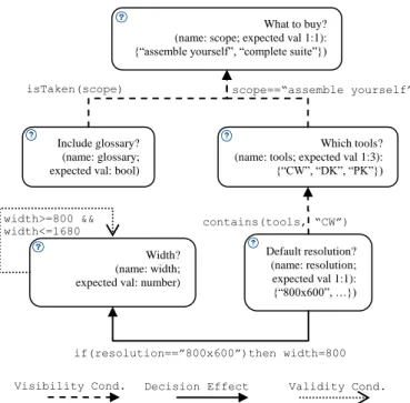
problem space. Fig. 1 depicts a small part of an existing DOPLER decision model that describes the variability of the DOPLER tool suite [11]. The tool suite mainly comprises three separate tools: DecisionKing (DK) supports variability modeling; ProjectKing (PK) supports preparing models for product derivation; and the ConfigurationWizard (CW) supports end-users in deriving and configuring products. The variability model allows creating different variants of the DOPLER tool suite as described in [11]. Depending on the selection of DOPLER tools to be deployed, specific configuration parameters need to be set for deriving the tool suite for an end-user. For example, setting the resolution in advance is only relevant for the CW tool.
Figure 1. Example of a simplified DOPLER decision model with five interdependent decisions.
The key concepts in the DOPLER language relevant for the purpose of verification are as follows (see [7] for details): The Decision Type defines the range of values which can be assigned to a decision. The decision types in DOPLER are Boolean, String, Number and Enumeration. Boolean decisions in DOPLER (cf. decision glossary in Fig. 1) can be set to true or false. String decisions can take any text as a value. Number decisions take a floating point value (cf. decision width in Fig. 1). Enumeration decisions have two or more (String) values to select from and a cardinality defining the minimum and maximum number of values to be selected. In the example shown in Fig. 1,
scope is an Enumeration decision with two possible values
(“assemble yourself”, “complete suite”) and a cardinality of 1:1. Decision Attributes are properties of decisions. For example, the question (“What to buy?”; cf. Fig. 1) is presented to the user when enacting the decision model during product derivation. A
description allows further documentation of the decision. Other attributes can be defined by the modeler.
A Visibility Condition defines for a decision when it becomes visible to the user during product derivation depending on values set to other decisions. For example, it does not make sense to ask a user about specific properties of the user interface of a tool (e.g., the resolution of the tool "CW"; cf. Fig. 1) if the user has not yet decided whether the CW tool should be part of the derived product. The visibility condition “true” of decision scope means that it becomes a “root decision” which is always visible during product derivation. The function isTaken is used to make a decision (e.g., glossary) visible as soon as another decision (e.g.,
scope) is taken regardless of its value.
Decision Effects specify dependencies between decisions as rules in an event condition action pattern (i.e., when a decision is taken and a certain condition is fulfilled, the specified actions are performed). This mechanism allows automatically setting values of other decisions depending on some condition. For example, a constraint in the form resolution==”800x600” implies
width==800 could be specified using the decision effect rule if (resolution==”800x600”) then width==800 (cf. Fig. 1).
A Validity Condition constrains the range of possible values for a particular decision. For example, a Number decision (e.g.,
width; cf. Fig. 1) can practically take any number as a value. By
defining a validity condition this range can be constrained, e.g., to only allow values between 800 and 1680.
An asset model defines the reusable assets of a product line and the dependencies among them. Fig. 2 depicts an example using the asset types Plug-in and Setting which are required in the DOPLER tool suite [11].
Plugin
-name : string = CW Plugin
-inclusion condition : string = contains(tools, "CW") -description : string = ...
-location : string = svn://...
Plugin
-name : string = Glossary Plugin -inclusion condition : string = glossary == true -description : string = ...
-location : string = svn://...
Plugin
-name : string = Core Plugin -inclusion condition : string = true -description : string = ... -location : string = svn://...
Setting
-name : string = Resolution width -inclusion condition : string = isTaken(width) -description : string = ...
-width_value : string = width <<requires>> <<requires>>
<<contributes to>>
Figure 2. A partial DOPLER asset model depicting a small set of assets, their attributes, and relationships between them. The inclusion conditions refer to the decisions from Fig. 1. Asset Attributes are used to define properties of an asset, like its name and description. For instance, in Fig. 2 the asset CW Plugin of asset type Plugin has the additional attribute location and the asset Resolution width of asset type Setting has the additional attribute width_value.
Asset Dependencies define relationships between assets. Arbitrary relationship types with different semantics [7] can be predefined in DOPLER meta-models to enable modeling structural or functional dependencies. Examples of possible
What to buy? (name: scope; expected val 1:1): {“assemble yourself”, “complete suite”})
Which tools? (name: tools; expected val 1:3): {“CW”, “DK”, “PK”}) Include glossary?
(name: glossary; expected val: bool)
Default resolution? (name: resolution; expected val 1:1): {“800x600”, …}) isTaken(scope) contains(tools, “CW”) Width? (name: width; expected val: number)
Validity Cond. Visibility Cond. Decision Effect
if(resolution==”800x600”)then width=800 width>=800 &&
width<=1680
relationships are requires, contributes to or implements. For instance, the asset CW Plugin requires the Core Plugin and the
Resolution width setting contributes to CW Plugin.
Inclusion Conditions link assets to decisions. They describe for an asset under which condition it is part of the derived product. One asset can depend on the values of multiple decisions and arbitrary conditions can be defined. For instance, the asset CW
Plugin is included if the set of values for Enumeration decision tools (cf. Fig. 1) contains the value CW. This means that the asset
is included if the answer to the decision is CW, but also in the cases (CW, DK); (CW, PK); or (CW, DK, PK).
3. REPRESENTING DOPLER MODELS AS
CONSTRAINT PROGRAMS
Creating a constraint-based representation of DOPLER models allows us to implement automatic reasoning operations (here: verification) on DOPLER variability models. We use the constraint solver GNU Prolog [6] but other solvers may also be used to execute these operations, if they support Boolean and arithmetic constraints over integer values (an example would be Choco [13]). Product line requirements can be easily expressed in terms of constraints over integers. We decided to use GNU Prolog to solve the resulting constraints for several reasons: (i) constraints can be expressed in a very declarative way [17] thanks to the Prolog layer and to a wide variety of predefined constraints; (ii) the GNU Prolog constraint solver is very efficient; and (iii) this system is developed by our team.
3.1 Background: Constraint Programming
Constraint Programming (CP) emerged in the 1990’s as a paradigm to tackle complex combinatorial problems in a declarative manner [22]. CP extends programming languages with the ability to deal with undefined variables of different domains (e.g. Integers, Reals, Booleans, ...) and specific declarative relations between these variables called constraints. Constraints are solved by specialized algorithms which are adapted to their specific domains and therefore can be much more efficient than generic logic-based engines. A constraint is a logical relationship among several unknowns (or variables) each one taking a value in a given domain of possible values. A constraint thus restricts the possible values that variables can take. A Constraint Satisfaction Problem (CSP) is defined as a triple (X, D, C), where X is a set of variables, D is a set of domains, i.e., finite sets of possible values (one domain for each variable), and C is a set of constraints restricting the values that the variables can take simultaneously. Classical CSPs usually consider finite domains for the variables (Integers) and solvers use propagation-based methods [3, 22]. Such solvers keep an internal representation of variable domains and reduce them monotonically to maintain a certain degree of consistency with regard to the constraints. In modern CP languages [6, 19], many different types of constraints exist and are used to represent real-life problems: arithmetic constraints, e.g., X * Y < Z, meaning that the resulting value of X multiplied
by Y must be less than the value of Z; symbolic constraints, e.g., atmost(N, [X1,X2,X3],V), meaning that at most N variables
among [X1, X2, X3] can take the value V; global constraints, e.g., all different(X1, X2, …,Xn), meaning that all variables should have different values; and reified constraints (e.g., BoolExpr1
==> BoolExpr2 constrains BoolExpr1 to imply BoolExpr2 allows
the user to reason about the truth value of a constraint).
Solving constraints is done by first reducing the variable domains by propagation techniques to eliminate inconsistent values within domains. This is followed by finding values for each constrained variable in a labeling phase. Variables are grounded iteratively by fixing a value and propagating its effect onto other variable domains (again applying the same propagation-based techniques). The labeling phase can be improved using heuristics concerning the order in which variables are considered as well as the order in which values are tried in the variable domains.
3.2 Converting DOPLER Models to
Constraint Programs
Constraint programs (CPs) are represented by variables and relationships among them [17]. For representing DOPLER as constraint programs, we first need to identify the DOPLER model elements defining the variability of a product line as only those are relevant in this case. Attributes like the description attribute of an asset or a decision do not affect variability and can thus be ignored in the constraint representation. The representation of DOPLER models as constraint programs hence has the following properties:
Each decision will be represented as a CP variable
Each asset will be represented as a CP variable.
Let D be a decision with a visibility condition. If the
visibility condition indicates that the decision is not
visible, the corresponding variable is assigned with
zero (0). If the visibility condition is a formula, the
variable representing the decision is assigned with
that particular formula. If the visibility condition
indicates that the decision is always visible, the
variable representing the decision is affected with
one (1). If the visibility condition of the decision D
is not defined, its domain is {0,1}.
For Number and String decisions the validity
condition becomes the domain of variables
representing these decisions. The domains of all
variables are finite and must be composed of integer
values.
The domain of Boolean and Enumeration decisions
is mapped into a {0,1} domain. Zero indicates that
nothing has been selected and one indicates the
selection of the associated variable.
The domain of assets is mapped into a {0, 1}
domain. If the variable representing an asset takes
the value 0 in a configuration process it means that
the asset is not included. If it takes the value 1, the
asset will be included in a derived product.
Asset dependencies are described as constraints.
Decisions, assets, and dependencies among them
can be mapped into CPs by using the following
rules.
Decision type and validity condition: Let D be a decision, type be its type and valc its validity condition. If D.type = Boolean or
Enumeration then the equivalent constraint is D ∈ {0, 1}. If
valc. Note that the validity condition of String decisions must be
previously represented as integer values. For example, a String decision with validity condition valc = {Sunday, Monday, Tuesday} can be represented as valc={1, 2, 3}, where 1 means Sunday, etc. If D.type = Enumeration, let <m, n> be its cardinality and DOpt1, DOpt2, ..., DOpti, a set of i decision
options grouped in cardinality <m, n>. Then the corresponding constraint is: DOpt1 ∈ {0, 1} ˄ DOpt2 ∈ {0, 1}˄, ..., DOpti∈ {0,
1} ˄ D ⇔ m ≤ DOpt1 + DOpt2 + ...+ DOpti ≤ n.
Visibility condition: Let D be a decision and visc its visibility condition. If visc = false then D = 0. If visc = true then D =1. If
visc is a different expression, then the corresponding constraint is: D ⇒ visc. Note that a visibility condition (i.e., visc) can be true, false or depending on one or more decisions and their values (e.g., scope==“assemble yourself” or isTaken(scope)).
Decision Effects: Let D be a decision and df its decision effect. The corresponding constraint is: D ⇒ df.
Asset Inclusion Conditions: Let A be an asset and ic its inclusion condition. The corresponding constraint is: A ⇒ ic.
Asset Dependencies: Let A be an asset, ad its dependency and
type its type. If type is “requires”, the corresponding constraint is: A ⇒ ad. If type is “excludes”, the corresponding constraint is: A * ad = 0. This means that if A is selected (equal to 1), ad must not
be selected (must be equal to 0) and vice-versa. Currently, we do not take into account other types of asset dependencies (like parent or child).
The conversion algorithm has two main phases presented in the following pseudo-code (Algorithm 1). First, the algorithm navigates through the decision model and then through the asset model. In both cases, we gather the relevant information of decisions and assets and translate them into constraints in CP. Relevant information means information affecting the variability as described above; for example, a description attribute does not affect the variability of the product line model. Our algorithm for converting DOPLER variability models is implemented as an Eclipse plug-in that uses the API of the DOPLER tool suite [8].
Algorithm 1. Our algorithm for converting DOPLER models to constraint programs. The variable DM represents the
DOPLER model to be transformed and the variable CP accumulates the results of each transformation. CP is the
resulting constraint program representing DM.
CP = "";
for each decision D in DM{ if D.type == Boolean { CP += "D ∈ {0, 1}";
visc = D.getVisibilityCondition(); if visc == false { CP += "D = 0";} else if visc == true {CP += "D = 1";} else { CP += "D ⇒ visc";}
df = D.getDecisionEffect(); CP += "D ⇒ df";
}
else if D.type == Enumeration { CP += "D ∈ {0, 1}"; m, n = D.getCardinality(); DOpt1, DOpt2,...,DOpti=D.getDecOptions(); CP += "DOpt1, DOpt2,...,DOpti ∈ {0, 1}"; CP += "D ⇔ m≤DOpt1+DOpt2+...+DOpti≤n"; visc = D.getVisibilityCondition(); if visc == false { CP += "D = 0";} else if visc == true {CP += "D = 1";} else { CP += "D ⇒ visc";}
df = D.getDecisionEffect(); CP += "D ⇒ df";
}
else if D.type == Number {
val = representValidityConditionAsCP(); CP += "D ∈ val";
visc = D.getVisibilityCondition(); if visc == false { CP += "D = 0";} else if visc == true {CP += "D = 1";} else { CP += "D ⇒ visc";}
df = D.getDecisionEffect(); CP += "D ⇒ df";
}
else if D.type == String {
valc = representValidityConditionAsCP(); CP += "D ∈ valc";
visc = D.getVisibilityCondition(); if visc == false { CP += "D = 0";} else if visc == true {CP += "D = 1";} else { CP += "D ⇒ visc";}
df = D.getDecisionEffect(); CP += "D ⇒ df";
} }
for each asset A in DM{ CP += "A ∈ {0, 1}"; ic = A.getInclusionCondition(); if ic is not null { CP += "A ⇒ ic"; } ad = A.getDependency(); if A.type == requires { CP += "A ⇒ ad"; }
else if A.type == excludes { CP += "A * ad = 0"; }
}
Write ("The constraint program representation of the DOPLER model DM is: " + CP);
4. FORMAL VERIFICATION OF DOPLER
MODELS
The automated verification of DOPLER variability models has the goal to find defects and its sources using automated and efficient mechanisms. As the manual verification of variability models is error-prone and tedious we propose an automated solution. Our approach offers a collection of operations which are applied on a DOPLER model and return the evaluation results intended by the operation. We use a product line model of the
DOPLER tool suite (cf. Fig. 1 and Fig. 2) [11] as an example to illustrate our approach. The currently supported operations are: Void model. A model is void and useless if it defines no products at all. The void model operation returns true if the model is void or false otherwise. Several methods have been proposed to check for void models [21, 2, 20, 15]. Our approach determines if there is at least one configuration that can be generated based on the defined decisions. If the model is not void our constraint solver will give us the first configuration.
The example model (cf. Fig. 1 and 2) is not void because it can generate at least one product (e.g., if the scope decision is taken, the option “complete suite” is selected and the decision glossary is resolved to true, one product thus may be {Glossary Plugin,
Core Plugin}). Otherwise, if the visibility condition of the root
decision scope (first and only decision visible at the beginning when starting product derivation) is set to false, then no other decisions will become visible and answerable and therefore no products can be derived (the model would be void in this case). Non-attainable validity conditions’ and domains’ values. This operation either (i) takes a collection of decisions as input and returns the decisions that cannot attain one or more values of its validity condition or (ii) takes a collection of assets as input and returns the assets that cannot attain one of the values of its domain. A non-attainable value of a validity condition or a domain is a value that can never be taken by a decision or an asset in a valid product. Non-attainable values are undesired because they give the user a wrong idea of the values that decisions and assets modeled in the product line model can take.
In our example (cf. Fig. 1) the decision effect of the decision
resolution is if resolution == 800X600 then width = 800. The
validity condition of width is width ≥ 800 && width≤1680. In this example some values of width’s validity condition can never be taken, for example: 801 to 1023, 1025, etc. Thus, in this case, constraining the values of width to “width ≥ 800 &&
width≤1680” gives a wrong idea of the values that decision width
can take. Instead, a more precise definition of the domain value of
width would thus be {800, 1024, …}.
Dead decisions and assets [21, 20, 24, 26]. This operation takes a collection of decisions and assets as input and returns the set of dead decisions and assets (if some exist) or false otherwise. A decision is dead if it never becomes available for answering it. An asset is dead if it cannot appear in any of the products of the product line. The presence of dead decisions and assets in product line models indicates modeling errors and intended but unreachable options. A decision can become dead (i) if its visibility condition can never evaluate to true (e.g., if contradicting decisions are referenced in a condition); (ii) a decision value violates its own visibility condition (e.g., when setting the decision to true will in turn make the decision invisible); or (iii) its visibility condition is constrained in a wrong way (e.g., > 5 && < 3). An asset can become dead (i) if its inclusion depends on dead decisions, or (ii) if its inclusion condition is false and it is not included by other assets (due to
requires dependencies to it). Dead variables in CP are variables
than can never take a valid value (defined by the domain of the variable) in the solution space. Thus, our approach consists in evaluating each non-zero value of each variable’s domain. If a variable cannot attain any of its non-zero values, the variable is
considered dead. The zero value of a CP variable in the domain of product lines means that this variable has not been selected. In our example (cf. Fig. 1 and 2) if the visibility condition of the decision glossary is set to false by the modeler (zero in CP) then the related asset Glossary Plugin will never be selected for any product during product derivation.
Redundant relationships. This operation takes a relationship as input and returns true if removing the relationship does not change the space of possible solutions. Redundant relationships in product line models should be avoided as they do not alter the space of possible solutions while increasing computational effort in derivation and analysis [25] as well as maintenance effort during product line evolution. One way to identify redundant relationships is to calculate all possible products for a given DOPLER model including a specific relationship to be checked for redundancy and then to remove the relationship and re-calculate all possible products using the changed model. If the results are equal and the same set of products are created before and after the elimination then the relationship can be considered redundant. This approach would however by very expensive and often infeasible. We thus find redundant relationships based on the fact that if a constraint program is consistent, then the constraint program plus a redundant constraint is consistent too. Therefore, denying the supposedly redundant relationship implies contradicting the consistency of the constraint program and then to make it inconsistent. For example, if a system where A requires
B and B requires C is consistent, then the constraint A requires C
is redundant and reaffirms the consistency of the original system. If instead of the constraint A requires C, we put its negation; the system becomes inconsistent and therefore without solution. We decided to implement this approach because it is more efficient and thus more scalable even in very large models due to the backtracking algorithm provided by the solver we use [6]. In our example (cf. Fig. 1) an additional decision core (not in Fig. 1) might be added offering the choice of including the asset
Core Plugin (cf. Fig. 2) for products. If other assets include it
anyway (for all configurations) through a requires dependency the new decision would be redundant.
5. PRELIMINARY EVALUATION
We tested the feasibility of our verification approach with two existing DOPLER variability models. The first model is a variability model of the DOPLER tool suite which has already been used as an example throughout this paper. This model represents the variability of the configurable DOPLER tool suite and comprises 14 decisions and 67 assets. The model has been created by the developers of the DOPLER tool suite. The second model defines the variability of a fictitious product line of digital cameras. This model has been created by analyzing datasheets of all available digital cameras of a well-known digital camera manufacturer. The model comprises 7 decisions and 32 assets. In our preliminary evaluation we seeded 33 defects in the DOPLER model and 22 defects in the camera model. The defects cover different types of problems to show the feasibility of the verification approach. For instance, the decision Wizard_height cannot take the values 1200, 1050, 1024 and 768 and the asset
VAI_Configuration_DOPLER cannot take the value 1 (is never
corresponding variables’ domain. Furthermore, we measured the execution time of applying the approach for both models for the different types of analyses.
Applying our verification approach to the DOPLER model has shown that the model is not void and can generate 23016416 products. However, we discovered 18 defects related with non-attainable domain values and 15 dead decisions and assets (these together are the 33 defects we have seeded before). By applying our verification approach on the digital camera model we obtained that the model is not void and can generate 442368 products. In this model, we discovered 11 defects related with non-attainable domain values as well as 11 dead decisions and assets (these together are the 22 defects we have seeded before). It is noteworthy that the same number of defects was identified in a manual verification of both models. The automated verification found all of the seeded defects in the DOPLER model and all of the seeded defects in the camera model.
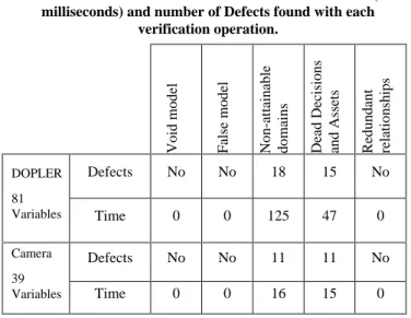
Table 1 shows the number of defects found and the execution time (in milliseconds) corresponding to the verification operations on the models. No defects were found regarding the “Void model”, “False model” and “Redundant relationships” operations and the execution time was less than 1 millisecond for each one of these operations in each model. Our solver does not provide time measures of microseconds (10-6 seconds); thus, 0 milliseconds (10-3 seconds) must be interpreted as less than 1 millisecond. The model transformations from DOPLER models to constraint programs took about 1 second for each model. Our verification approach is fully automated with our Eclipse plug-in for verification and analysis of constraint-based variability models [14].
Table 1. Results of model verifications: Execution time (in milliseconds) and number of Defects found with each
verification operation. Void mode l False mode l Non -at ta ina ble doma ins Dea d Dec isions and As sets Redunda nt re la ti onships DOPLER 81 Variables Defects No No 18 15 No Time 0 0 125 47 0 Camera 39 Variables Defects No No 11 11 No Time 0 0 16 15 0
6. DISCUSSION & OPEN ISSUES
The digital camera model (39 model elements) and DOPLER tool suite model (81 model elements) are rather small and of different size. In both cases, none of the operations took longer than 125 milliseconds to be executed. The good performance and scale of performance of the verifications in these two models indicate scalability for larger models. However, a validation with a case study to analyze the computational complexity of our approach
remains as future work. In addition, we plan to work on (i) the identification of additional and more specific verification criteria for DOPLER models to complement the rather generic checks proposed in this paper; (ii) support for the identification of the sources of defects found in verification operations like void
models or redundant relationships; (iii) explanations for the
defects found. For example, our approach allows identifying dead decisions and assets but does not provide any explanation about why this is an anomaly, how bad it is or what the scope of the anomaly in the model is; and (iv) providing fixing strategies for the identified defects.
7. ACKNOWLEDGMENTS
This work was partially funded by the Intra-European Fellowship “Bourse de mobilité Île de France” and the French Minister of Higher Education and Research. This work was also supported by the Christian Doppler Forschungsgesellschaft, Austria and Siemens VAI Metals Technologies.
8. REFERENCES
[1] D. Benavides, S. Segura, and A. Ruiz-Cortés, "Automated analysis of feature models 20 years later," Information
Systems, vol. 35(6), pp. 615–636, 2010.
[2] D. Benavides, A. Ruiz-Cortes, and P. Trinidad, "Automated reasoning on feature models, "Proc. of the 17th International
Conference on Advanced Information Systems Engineering (CAiSE 2005), Springer-Verlag, 2005, pp. 491-503.
[3] C. Bessiere. Constraint propagation. In Francesca Rossi, Peter van Beek, and Toby Walsh, editors, Handbook of Constraint Programming, pp. 29-83. Elsevier, 2006.
[4] G. H. Campbell, Jr., S. R. Faulk, D. M. Weiss. Introduction
To Synthesis. INTRO_SYNTHESIS_PROCESS-90019-N,
Software Productivity Consortium, Herndon, VA, USA, 1990.
[5] K. Czarnecki, U. W. Eisenecker. Generative Programming:
Methods, Techniques, and Applications. Addison-Wesley,
2000.
[6] D. Diaz, C. Philippe. Design and implementation of the GNU Prolog System. Journal of Functional and Logic Programming, 2001(6), 2001. http://www.gprolog.org. [7] D. Dhungana, P. Heymans, and R. Rabiser, "A Formal
Semantics for Decision-oriented Variability Modeling with DOPLER, "Proc. of the 4th International Workshop on
Variability Modelling of Software-intensive Systems (VaMoS 2010), Linz, Austria, ICB-Research Report No. 37,
University of Duisburg Essen, 2010, pp. 29-35.
[8] D. Dhungana, R. Rabiser, P. Grünbacher, and T. Neumayer, "Integrated tool support for software product line engineering, "Proc. of the 22nd IEEE/ACM International
Conference on Automated Software Engineering (ASE'07),
Atlanta, Georgia, USA, ACM, 2007, pp. 533-534.
[9] D. Dhungana, P. Grünbacher, and R. Rabiser, "The DOPLER Meta-Tool for Decision-Oriented Variability Modeling: A Multiple Case Study," Automated Software
Engineering, 2010 (in press; doi:
[10] H. Gomaa. Designing Software Product Lines with UML. Addison-Wesley, 2005.
[11] P. Grünbacher, R. Rabiser, D. Dhungana, and M. Lehofer, "Model-based Customization and Deployment of Eclipse-Based Tools: Industrial Experiences, "Proc. of the 24th
IEEE/ACM International Conference on Automated Software Engineering (ASE 2009), Auckland, New Zealand,
IEEE/ACM, 2009, pp. 247-256.
[12] K. C. Kang, S. Cohen, J. Hess, W. Nowak, S. Peterson. Feature-oriented domain analysis (FODA) feasibility study. Technical Report CMU/SEI-90TR-21, Software Engineering Institute, Carnegie Mellon University, Pittsburgh, PA, USA, 1990.
[13] F. Laburthe. Choco: implementing a cp kernel. In CP00 Post Conference Workshop on Techniques for Implementing Constraint programming Systems (TRICS), Singapour, September 2000.
[14] R. Mazo, C. Salinesi, D. Diaz. VariaMos Eclipse plug-in. https://sites.google.com/site/raulmazo/.
[15] M. Mendonca and D. Cowan, "Decision-making coordination and efficient reasoning techniques for feature-based configuration," Science of Computer Programming, vol. 75(5), pp. 311-332, 2009.
[16] K. Pohl, G. Böckle, F. van der Linden. Software Product
Line Engineering: Foundations, Principles, and Techniques.
Springer, 2005.
[17] C. Salinesi, R. Mazo, D. Diaz, O. Djebbi. Using Integer Constraint Solving in Reuse Based Requirements Engineering. Proc. of the 18th IEEE International
Conference on Requirements Engineering (RE'10). Sydney,
Australia. IEEE, 2010, pp. 243-251.
[18] K. Schmid and I. John, "A Customizable Approach to Full-Life Cycle Variability Management," Journal of the Science of
Computer Programming, Special Issue on Variability
Management, vol. 53(3), pp. 259-284, 2004.
[19] C. Schulte, P. J. Stuckey. "Efficient constraint propagation engines," ACM Trans. Program. Lang. Syst., vol. 31(1), pp. 1-43, 2008.
[20] P. Trinidad, D. Benavides, A. Durán, A. Ruiz-Cortés, M. Toro, "Automated error analysis for the agilization of feature modeling," Journal of Systems and Software, vol. 81(6), pp. 883-896, 2008.
[21] P. van den Broek, I. Galvão, "Analysis of Feature Models using Generalised Feature Trees," Proc. of the Third
International Workshop on Variability Modelling of Software-intensive Systems (VaMoS 2009), Sevilla, Spain,
University Duisburg-Essen, ICB-Research Report No. 29, 2009, pp. 29-36.
[22] P. Van Hentenryck. Constraint Satisfaction in Logic
Programming. The MIT Press, 1989.
[23] M. Vierhauser, P. Grünbacher, A. Egyed, R. Rabiser, and W. Heider, "Flexible and Scalable Consistency Checking on Product Line Variability Models, "Proc. of the 25th
IEEE/ACM International Conference on Automated Software Engineering (ASE 2010), Antwerp, Belgium, ACM, 2010,
pp. 63-72.
[24] T. von der Maßen and H. Lichter, "Deficiencies in Feature Models, "Proc. of the Workshop on Software Variability
Management for Product Derivation - Towards Tool Support, held in conjunction with SPLC 2004 - 3rd Software
Product Line Conference, Boston, MA, USA, 2004, pp. 14. [25] H. Yan, W. Zhang, H. Zhao, H. Mei, "An optimization
strategy to feature models’ verification by eliminating verification-irrelevant features and constraints," Proc. of the
11th International Conference on Software Reuse (ICSR 2009), Falls Church, VA, USA, Springer, 2009, pp. 65-75.
[26] W. Zhang, H. Zhao, H. Mei, "A propositional Logic-based Method for Verification of Feature Models," Proc. of the 6th
International Conference on Formal Engineering Methods ( ICFEM), Seattle, WA, USA, Springer, 2004, pp. 115-130.