HAL Id: hal-03111011
https://hal.archives-ouvertes.fr/hal-03111011
Submitted on 15 Jan 2021
HAL is a multi-disciplinary open access
archive for the deposit and dissemination of
sci-entific research documents, whether they are
pub-lished or not. The documents may come from
teaching and research institutions in France or
abroad, or from public or private research centers.
L’archive ouverte pluridisciplinaire HAL, est
destinée au dépôt et à la diffusion de documents
scientifiques de niveau recherche, publiés ou non,
émanant des établissements d’enseignement et de
recherche français ou étrangers, des laboratoires
publics ou privés.
around the Arabian Peninsula
Efstratios Bourtsoukidis, Lisa Ernle, John N. Crowley, Jos Lelieveld,
Jean-Daniel Paris, Andrea Pozzer, David Walter, Jonathan Williams
To cite this version:
Efstratios Bourtsoukidis, Lisa Ernle, John N. Crowley, Jos Lelieveld, Jean-Daniel Paris, et al..
Non-methane hydrocarbon (C2–C8) sources and sinks around the Arabian Peninsula. Atmospheric
Chem-istry and Physics, European Geosciences Union, 2019, 19 (10), pp.7209-7232.
�10.5194/acp-19-7209-2019�. �hal-03111011�
https://doi.org/10.5194/acp-19-7209-2019 © Author(s) 2019. This work is distributed under the Creative Commons Attribution 4.0 License.
Non-methane hydrocarbon (C
2
–C
8
) sources and sinks around
the Arabian Peninsula
Efstratios Bourtsoukidis1, Lisa Ernle1, John N. Crowley1, Jos Lelieveld1, Jean-Daniel Paris2, Andrea Pozzer1, David Walter3, and Jonathan Williams1
1Department of Atmospheric Chemistry, Max Planck Institute for Chemistry, Mainz 55128, Germany
2Laboratoire des Sciences du Climat et de l’Environnement, CEA-CNRS-UVSQ, UMR8212, IPSL, Gif-sur-Yvette, France 3Department of Multiphase Chemistry, Max Planck Institute for Chemistry, Mainz 55128, Germany
Correspondence: Efstratios Bourtsoukidis (e.bourtsoukidis@mpic.de)
Received: 29 January 2019 – Discussion started: 14 February 2019
Revised: 25 April 2019 – Accepted: 29 April 2019 – Published: 29 May 2019
Abstract. Atmospheric non-methane hydrocarbons (NMHCs) have been extensively studied around the globe due to their importance to atmospheric chemistry and their utility in emission source and chemical sink identification. This study reports on shipborne NMHC measurements made around the Arabian Peninsula during the AQABA (Air Quality and climate change in the Arabian BAsin) ship campaign. The ship traversed the Mediterranean Sea, the Suez Canal, the Red Sea, the northern Indian Ocean, and the Arabian Gulf, before returning by the same route. The Middle East is one of the largest producers of oil and gas (O&G), yet it is among the least studied. Atmospheric mixing ratios of C2–C8 hydrocarbons ranged from a few
ppt in unpolluted regions (Arabian Sea) to several ppb over the Suez Canal and Arabian Gulf (also known as the Persian Gulf), where a maximum of 166.5 ppb of alkanes was detected. The ratio between i-pentane and n-pentane was found to be 0.93 ± 0.03 ppb ppb−1 over the Arabian Gulf, which is indicative of widespread O&G activities, while it was 1.71 ± 0.06 ppb ppb−1 in the Suez Canal, which is a characteristic signature of ship emissions. We provide evidence that international shipping contributes to ambient C3–C8 hydrocarbon concentrations but not to
ethane, which was not detected in marine traffic exhausts. NMHC relationships with propane differentiated between alkane-rich associated gas and methane-rich non-associated gas through a characteristic enrichment of ethane over propane atmospheric mixing ratios. Utilizing the variability– lifetime relationship, we show that atmospheric chemistry governs the variability of the alkanes only weakly in the
source-dominated areas of the Arabian Gulf (bAG=0.16)
and along the northern part of the Red Sea (bRSN=0.22), but
stronger dependencies are found in unpolluted regions such as the Gulf of Aden (bGA=0.58) and the Mediterranean Sea
(bMS=0.48). NMHC oxidative pair analysis indicated that
OH chemistry dominates the oxidation of hydrocarbons in the region, but along the Red Sea and the Arabian Gulf the NMHC ratios occasionally provided evidence of chlorine radical chemistry. These results demonstrate the utility of NMHCs as source/sink identification tracers and provide an overview of NMHCs around the Arabian Peninsula.
1 Introduction
Anthropogenic activities are estimated to be responsible for the release of 169 Mt of non-methane hydrocarbons (NMHCs) into the atmosphere each year (Huang et al., 2017). NMHCs are important in atmospheric chemistry as precursors of tropospheric ozone and particle formation, both of which have negative impacts on air quality, human health, and climate (Lelieveld et al., 2015; Seinfeld and Pandis, 2016; EEA, 2018). Ozone production is known to be efficient in Oil and Gas (O&G) basins (Edwards et al., 2014; Wei et al., 2014; Field et al., 2015) when the high NMHC concen-trations react with the hydroxyl radical (OH) under low ni-trogen oxide (NOx) regimes leading to carbonyls which
pho-tolyse to recycle the OH oxidant (Rohrer et al., 2014). Since ozone production is photochemical and catalysed by NOx,
el-evated ozone concentrations (Parrish et al., 2004; Lelieveld et al., 2009; Perring et al., 2013; Helmig et al., 2014).
Globally, NMHC sources are dominated by urban centres. Road transportation (including both evaporative and com-bustion emissions), residential comcom-bustion, transformation industry, fuel production and transmission, and solvent use contribute about three-quarters to the estimated global total (Huang et al., 2017). Biomass burning (Andreae and Crutzen, 1997; Pozzer et al., 2010) in addition to biogenic sources (Poisson et al., 2000; Pozzer et al., 2010) and the Earth’s degassing (Etiope and Ciccioli, 2009) complete the diverse and dynamic inventory of NMHC sources. The dynamic na-ture of the NMHC source strength and hydrocarbon composi-tion is driven by political, socioeconomic, and environmental decisions. For example, reducing petrol- and diesel-powered vehicles can result in an overall decrease in transportation sector emissions but an increase in the share of alkanes in the summed emission NMHC (Huang et al., 2017). The general decline in fossil fuel usage had led to decreasing trends of global ethane concentrations (Aydin et al., 2011), but the de-mand for cleaner-than-coal burning energy resulted in an ex-pansion of natural gas production in the US (Swarthout et al., 2013) and reversal of global atmospheric ethane and propane trends due to US O&G activities (Helmig et al., 2016).
Since most sources have distinct emission composition patterns, hydrocarbon ratios are frequently used for identi-fication and characterization of sources. The isomeric pen-tane ratio (i-penpen-tane / n-penpen-tane) has been used to charac-terize vehicle emissions, gasoline, O&G activities, and ur-ban conditions in general (Gilman et al., 2013; Thompson et al., 2014; Baker et al., 2008). Correlations with propane, which is usually associated with natural gas processing and petroleum refining, can serve as an indicator of local/regional emission sources (Swarthout et al., 2013; Helmig et al., 2016), while the relative methane abundance can provide an indication of the type of gas (associated or non-associated with liquids) responsible for the emissions (Farry, 1998; Salameh et al., 2016).
Due to their relatively short atmospheric lifetimes that range from a few hours to several weeks, the variability of the NMHC mixing ratios can serve to determine to what degree sources and sinks impact the measurements on a regional scale. Based on the Junge relationship (Junge, 1974), Job-son et al. (1998) established a correlation between the natu-ral logarithm of the standard deviation of the gas concentra-tions and the chemical lifetimes for shorter-lived gases such as NMHCs. This variability–lifetime relationship has been applied in characterizing the impact of chemistry at various locations (Jobson et al., 1999; Williams et al., 2000, 2001; Bartenbach et al., 2007; Helmig et al., 2008). In addition, the presence of specific oxidants can be detected by the use of NMHC oxidative pairs (Parrish et al., 2007; Baker et al., 2016; Young et al., 2014). This is particularly important for Cl radicals as there is no instrumentation available for direct
Cl measurements, although measurements of ClNO2indicate
a Cl source to be present.
The objective of this study is to present a comprehensive assessment of the atmospheric mixing ratios of the NMHCs that were measured in the marine boundary layer across the Mediterranean Sea and around the Arabian Peninsula dur-ing the AQABA (Air Quality and climate change in the Ara-bian BAsin) ship campaign. NMHCs are used to character-ize the various emission sources encountered (including ship, O&G, regional, and urban emissions) and to evaluate at-mospheric oxidation processes (by using lifetime–variability and selected oxidative pair relationships). Specific sources and sinks are studied by analysing NMHC mixing ratios in the extremely clean and polluted conditions encountered within this rarely investigated region.
2 Methods
2.1 The AQABA ship campaign
To study the Air Quality and Climate in the Arabian BAsin, AQABA, a suite of gas-phase and aerosol instruments was installed inside five air-conditioned laboratory containers and set onboard the Kommandor Iona (KI) research ves-sel (IMO: 8401999, flag: UK, length overall × breadth ex-treme: 72.55 m × 14.9 m). The shipborne measurement cam-paign lasted from the beginning of July to the end of August 2017, starting from the south of France, across the Mediter-ranean Sea, and through the Suez Canal to Kuwait and back, covering around 20 000 km at sea (Fig. 1) at an average speed of 3.4 ± 1.8 m s−1. When possible, in order to reduce sampling of its own exhaust, the ship sailed upwind of the shipping lane and at an angle to the prevailing wind. Dur-ing the campaign, the average temperature was 30.6 ± 3.9◦C (range: 22.9–38.7◦C) and the average relative humidity was 71.4 ± 16.3 % (range 23.5–94.5 %), while the wind speeds encountered were on average 5.4 ± 2.8 m s−1 (range: 0.7– 14 m s−1).
2.2 Gas chromatography–flame ionization detector
2.2.1 Instrumentation
Non-methane hydrocarbons were measured with two cou-pled GC–FID systems (GC5000VOC and GC5000BTX; AMA Instruments GmbH, Germany). The GC5000VOC was used for the quantification of light hydrocarbons (C2–C6),
while the CG5000BTX was used for the heavier hydro-carbons and aromatics (C6–C8). Both systems share the
same operating principle as sample collection on absorbent-filled enrichment traps (Carbosieve/Carbograph 1 : 1 for AMA5000VOC and Carbotrap for AMA5000BTX), subse-quent thermal desorption, chromatographic separation (an-alytical column for GC 5000 VOC: AMA-sep Alumina, 0.32 mm ID, 50 m, 8 µm, and for GC5000BTX: AMA-sep1,
Figure 1. Back-trajectory calculations along the route which start at the ship position and follow air masses back in time for 4 days on an hourly time grid.
0.32 mm ID, 30 m, 1.5 µm), and detection of the eluting trace gases by flame ionization detectors. Their main differ-ence is that the GC5000VOC system uses a dual-stage pre-concentration principle, additionally equipped with a second trap (focusing trap/Carbosieve/Carbograph 1 : 1) and a sec-ond chromatographic column (AMA-sep WAX, 0.32 mm ID, 30 m, 0.25 µm) in order to improve injection, peak resolution, and chromatographic separation.
To enable stand-alone combustion and carrier gas supply without the use of additional high-pressure gas cylinders, a hydrogen generator (H2PD-300-220, Parker Hannifin Corpo-ration, USA) and zero air generator (AK6.1, Innotec GmbH & Co. KG, Germany) were operated in parallel. The zero air generator was supplied with compressed air (Compressor UA-025K/05641100, Dürr Technik GmbH & Co. KG, Ger-many) at 2 bar, after three-stage filtering through cartridges filled with different adsorbent materials. The first cartridge is filled with silica gel for drying, the second with charcoal for ozone and particle removal, and the third with a mixture of charcoal, molecular sieve, and soda lime for CO2and organic
trace gas removal. Inside the zero air generator, a palladium catalyst is heated to 430◦C to eliminate any remaining hy-drocarbons and carbon monoxide. The zero air produced was used for both FID flames in addition to the Nafion drier.
2.2.2 Water and ozone interferences
The necessity of water and ozone removal in NMHC quan-tification has been frequently reported in the literature (Helmig and Greenberg, 1995; Plass-Dülmer et al., 2002; Slemr et al., 2002; Apel et al., 2003; Rappenglück et al., 2006). As the campaign was planned for the moist marine boundary layer and for areas that were likely to have high ambient ozone concentrations (Lelieveld et al., 2002, 2009), the effects of humidity and ozone were studied in the labora-tory prior to deployment.
Moist air (relative humidity 100 %) substantially influ-enced ethene concentrations compared to dry air (increased by a factor of 2.2), while it had a smaller effect on propene
(increased by a factor of 1.16), benzene (increased by a factor of 1.28), and all other species (differences below ±10 % be-tween dry and moist air). The use of the Nafion drier (Perma Pure LLC) effectively eliminated these discrepancies as it proved capable of drying the ingoing sample air without pro-ducing chromatographic artefacts for the NMHCs investi-gated.
Stepwise addition of O3 up to mixing ratios of 200 ppb
showed no significant impact of ozone on the alkane mea-surements. The most affected species were the alkenes and in particular isoprene, which decreased in mixing ratio by 25 % per 100 ppb of O3. Therefore two ozone scrubbers
were tested. The potassium iodine scrubbers (LpDNPH, Su-pelco Analytical, USA) showed limited O3removal capacity
(ca. 45 L at 70 ppb O3) and induced chromatographic
arte-facts such as noisy background and ghost peaks. In con-trast, Na2S2O3-impregnated quartz filters removed O3 with
much larger capacity (> 200 L at 70 ppb O3) without
af-fecting the quality of the chromatograms. We therefore used the Na2S2O3-infused quartz filters for ozone removal in the
NMHC sampling.
2.2.3 Sampling
The GC–FID system was installed inside one of the five air-conditioned laboratory containers. A 5.5 m tall (3 m above the container), 0.2 m diameter, high-flow (≈ 10 m3min−1) stack was used as the common inlet for all gas-phase mea-surements. For NMHC sampling, a sub-flow of 2.5 L (stp) min−1 (Lpm) was drawn through a PTFE filter (5 µm pore size, Sartorius Corporate Administration GmbH, Germany) for particle removal and then through a heated (ca. 40◦C)
and insulated PFA-Teflon line (12 m length, OD = 0.635 cm) with a residence time of approximately 9 s. The PTFE filter was exchanged every 2–5 days depending on the aerosol and sea salt load encountered. Inside the container, the GC–FID systems sampled air from the main 2.5 L min−1 stream at a rate of 90 sccm (2 × 45 cm3(stp) min−1(sccm)), through an ozone scrubber (Na2S2O3-infused quartz filters) and a
Nafion dryer (500 sccm counter-flow) that were used to elim-inate the effects of ozone and humidity in sample collection. Similar to ambient samples, the calibration gas was passed through the ozone scrubber and Nafion dryer to ensure iden-tical calibration conditions through the complete campaign (Fig. S1 in the Supplement).
The broad range of NMHC concentrations encountered along the ship track dictated in situ adjustments in the sam-pling volume. It is worth noting that in addition to ambient concentrations, high waves that cause intense yaw, pitch, and roll movements of the ship can disturb flow controllers and influence the flame stability and signal baseline and hence detection limits. Therefore, depending on ambient NMHC concentrations and wave conditions, three sampling volumes were used throughout the campaign. In polluted conditions, such as the Arabian Gulf and the Suez Canal, short sampling times (10 min) and volumes (450 mL) allowed higher time resolution (50 min per measurement), while under clean con-ditions, such as found in the Arabian Sea, longer sampling times and volumes (30 min, 1350 mL, time resolution = 1 h) improved detection limits. For most of the route, the sam-pling time was 20 min, the samsam-pling volume 900 mL, and the time resolution 50 min per measurement.
Temperature control of the traps is done by Peltier ele-ments which permit rapid heating and cooling rates along with high temperature reproducibility. Sample collection was carried out at 30◦C for all traps, while desorption tempera-ture was 230◦C. The typical container temperature was about 25◦C and condensation was avoided with the use of heated lines and the Nafion drier. A different oven temperature pro-gramme of a 38 min cycle was selected for the two GC– FID systems. The initial oven temperatures were set to 50◦C
and 60◦C, while the final oven temperatures were 160◦C
and 200◦C for the GC5000VOC and GC5000BTX systems respectively. The detailed temperature programme for each GC–FID system can be seen in Fig. S2.
2.2.4 Calibrations
Frequent calibration and blank samples ensured optimum and stable performance of the GC–FID systems. A multi-component reference gas mixture (National Physical Labora-tory, UK, 2015) was diluted with synthetic air (6.0, Westfalen AG, Germany) and passed through both the ozone scrubber and the Nafion drier to provide sampling conditions similar to ambient air. In total, 79 calibration and 20 blank sples were obtained throughout the campaign. Prior to am-bient samples, a six-step calibration curve (6 × 3) was ob-tained for 450 and 900 mL sampling volumes, confirming the high sensitivity and excellent linearity of FID detectors as the R2of the linear fit for all species was always higher than 0.98. During the campaign, single calibration points and blanks were frequently obtained to monitor the sensi-tivity while minimizing data loss. Analysis of the initial cal-ibrations revealed volume-dependent sensitivity for ethane,
Table 1. Detection limits and total uncertainty of measured NMHCs. The average detection limits (DLs) for each compound are reported in the first column. DLs varied during the campaign as a result of different sampling volumes and wave height. The average total uncertainty was derived by error interpolation and is reported in the third column.
Compound DL DL range Total (ppt) (ppt) uncertainty (%) ethane 7 0.1–74 7.3 propane 3 0.3–31 7.2 i-butane (2-methylpropane) 2 0.2–19 8.9 n-butane (butane) 2 0.2–22 8.5 i-pentane (2-methylbutane) 2 0.2–25 9.9 n-pentane (pentane) 2 0.2–28 10.4 i-hexane (2-methylpentane) 2 0.6–43 6.3 n-hexane (hexane) 2 0.5–29 7.1 heptane 1 0.5–26 7.4 octane 1 0.5–14 7.7 ethene 25 1–150 12.5 propene 2 0.1–29 9.5 trans-2-butene (but-2-ene) 1 0.2–17 11 1-butene (but-1-ene) 1 0.1–12 12.4 benzene 2 0.6–26 7.3 toluene 2 0.5–21 8.3 m- + p-xylenes 3 1–48 8.6 (1,3- + 1,4-xylenes)
propane, ethene, and propene. Therefore, another set of linear calibrations with 1350 mL sampling volume was performed towards the end of the campaign. For the aforementioned species, the volume-dependent calibration curve was applied for deriving the ambient mixing ratios.
Due to varying baseline noise, dependent on the ship mo-tion, condition-specific detection limits (DLs) and total un-certainties have been calculated (Table 1). The limit of de-tection was calculated from the baseline noise, as this was determined by IAU Chrom integration software (Sala et al., 2014). Peaks that were higher than 3 times the noise signal were considered to be above DL. With this approach DLs for each calibrated chromatograph were derived. Similarly, a total uncertainty for each sample was derived. For the total uncertainty we propagated 5 % uncertainty in the measured flows combined with the % inherent reference gas mixture uncertainty and the varying peak uncertainty that was calcu-lated as the percentage signal-to-noise ratio for each chro-matographic peak.
2.2.5 Ship exhaust filter
During the complete ship campaign 1393 samples were col-lected by the GC5000VOC system and 1244 samples by the GC5000BTX system, resulting in 26 668 integrated peaks. For the purpose of this study, all samples that have been obtained in ports or under stationary conditions have been excluded from the analysis, with the only exception being the pentane mixing ratios measured in the Jeddah port (JP).
Similarly, samples influenced by the KI ship exhaust were considered only for the NMHC composition characteriza-tion and excluded from the ambient air assessments. To iden-tify which samples were affected by our own ship exhaust, a combination of wind direction relative to the ship movement and measured NO2, O3, and SO2was used to create a flag for
affected time frames. Since ethene mixing ratios were excep-tionally high inside the exhaust plume, as has been reported previously (Eyring et al., 2005), all flagged samples were in-dividually inspected for ethene, resulting in a filter that ex-cluded all samples that were contaminated by the emissions of the KI ship exhaust. Ethane was clearly not emitted by the KI ship exhaust, and therefore the filter was not applied for this particular hydrocarbon. The number of samples quanti-fied per measured species can be seen in Table 2.
2.3 Methane measurements
The CH4 molar mixing ratio was measured using a cavity
ring-down spectroscopy analyser (Picarro G2401). Four dif-ferent calibration gases traceable to WMO X2004A scale and bracketing typical ambient concentrations were injected into the analyser at ports and every 15 days for calibration pur-poses. The injection sequence consists of four 15 min injec-tions of each of the four gases. An additional target gas was injected daily to assess measurement accuracy. The data have been documented and processed following ICOS (Integrated Carbon Observing System) standard procedure (Hazan et al., 2016), including the propagation of the calibration and threshold-based filters. The mean drift of measured concen-trations from calibration cylinders between two sequences is 0.5 nmol mol−1, significantly below the drifts typically ob-served at fixed observatories (Hazan et al., 2016).
2.4 ECHAM5/MESSy Atmospheric Chemistry (EMAC) model
The ECHAM/MESSy Atmospheric Chemistry (EMAC) model is a numerical chemistry and climate simulation system that includes sub-models describing tropospheric and middle atmosphere processes and their interaction with oceans, land, and human influences (Jöckel et al., 2010). It uses the second version of the Modular Earth Submodel Sys-tem (MESSy2) to link multi-institutional computer codes. The core atmospheric model is the 5th generation Euro-pean Centre Hamburg general circulation model (ECHAM5, Roeckner et al., 2006). For the present study we applied EMAC (ECHAM5 version 5.3.02, MESSy version 2.53.0) in the T106L31 resolution, i.e. with a spherical truncation of T106 (corresponding to a quadratic Gaussian grid of ap-prox. 1.1 by 1.1◦in latitude and longitude) with 31 vertical hybrid pressure levels. A complex organic chemistry (MOM, Mainz Organic Mechanism) is integrated into the model as described in Sander et al. (2018). The simulation set-up is analogous to the one of Lelieveld et al. (2017).
2.5 Hybrid Single Particle Lagrangian Integrated Trajectory (HYSPLIT) model
Back-trajectories of air parcels encountered have been calcu-lated with the Hybrid Single-Particle Lagrangian Integrated Trajectory model (HYSPLIT, version 4, 2014), which is a hy-brid between a Lagrangian and an Eulerian model for trac-ing a small imaginary air parcel forward or back in time. The model can be accessed under https://ready.arl.noaa.gov/ HYSPLIT.php (last access: 20 May 2019), while further de-tails are provided in Draxler and Hess (1998). For the pur-poses of this study, back-trajectories with a start height of 200 m a.s.l. have been calculated, starting at the ship position and going back in time on an hourly time grid (Fig. 1).
3 Results and discussion
3.1 Overview of atmospheric mixing ratios
Widely varying mixing ratios of alkanes, alkenes, and aro-matics were quantified along both legs of the ship campaign (Figs. 2, S3–S19). To investigate regional variations in at-mospheric chemistry and abundance of NMHCs, the track was subdivided into eight regions: Mediterranean Sea (MS), Suez Canal (SC; including Great Bitter Lake and the Gulf of Suez), Red Sea North (RSN), Red Sea South (RSS), Gulf of Aden (GA), Arabian Sea (AS), Gulf of Oman (GO), and Arabian Gulf (AG) (for coordinates, see Table 2). Despite the leg-to-leg differences in the origin of the air masses (Fig. 1), ethane mixing ratios (Fig. 2) match well with this geograph-ical demarcation that has resulted in eight different regions.
The cleanest air masses were measured over the AS where the majority of NMHCs were below or close to the de-tection limit (Table 2). HYSPLIT back-trajectories (Fig. 1) show that these air masses sampled originated from the In-dian Ocean and were transported to the sampling point in the prevailing large-scale anticyclonic system. Land influ-ence was confined to a small part of the eastern Somali desert, where NMHC sources are negligible. Mean ethane mixing ratios over the AS were 0.26 ± 0.1 ppb on average, with the lowest recorded value being 0.16 ppb, an indica-tive value of the regional tropospheric background. Despite the small variability in comparison to the majority of the NMHCs measured (Fig. 3), ethene was found to be relatively high on average (0.09±0.06 ppb), with a maximum recorded value of 0.24 ppt. As ethene is highly reactive towards atmo-spheric oxidants and therefore has a short atmoatmo-spheric life-time (several hours), high mixing ratios are indicative of a local source. Ship traffic is unlikely to be the primary source of ethene in the AS region because of the low abundance of other ship-emission-related NMHCs.
Similar conditions were met over the MS, where ethene was 0.11 ± 0.04 ppb on average and with a 0.2 ppb maxi-mum. Nonetheless, average NMHC mixing ratios over the
Table 2. Spatial volume mixing ratio means, medians, standard deviations (SDs) and ranges of measured NMHCs.
Area Mediterranean Sea Suez Red Sea (N) Red Sea (S) Gulf of Aden Arabian Sea Gulf of Oman Arabian Gulf Coords start 35.959, 15.013 31.256, 32.354 27.821, 33.766 21.426, 38.972 12.553, 43.413 13.461, 50.142 22.869, 60.105 26.616, 56.566 (lat.(N), long.(E)) end 31.256, 32.354 27.821, 33.766 21.426, 38.972 12.553, 43.413 13.461, 50.142 22.869, 60.105 26.616, 56.566 29.381, 47.953
ethane N 125 90 210 113 116 262 104 162 mean (ppb) 0.90 2.46 3.03 0.67 0.44 0.26 0.55 7.82 median (ppb) 0.88 1.58 2.21 0.54 0.43 0.24 0.42 3.75 SD (ppb) 0.35 2.93 2.79 0.30 0.12 0.10 0.39 9.98 range (ppb) 0.51–4.17 0.27–21.59 0.46–17.33 0.45–1.97 0.27–1.11 0.16–1.34 0.23–2.43 0.4–48.02 propane N 125 76 189 98 75 178 86 157 mean (ppb) 0.37 3.86 1.71 0.25 0.17 0.11 0.55 7.93 median (ppb) 0.26 1.40 1.17 0.18 0.13 0.11 0.36 2.98 SD (ppb) 0.76 6.15 1.65 0.21 0.17 0.10 0.56 10.50 range (ppb) 0.03–8.61 0.11–32.16 0.13–10.45 0.07–1.06 0.03–1.35 0.01–1.16 0.06–2.94 0.31–53.79 i-butane N 125 76 189 98 72 133 83 158 mean (ppb) 0.05 1.39 0.39 0.09 0.03 0.005 0.20 2.90 median (ppb) 0.03 0.50 0.25 0.05 0.01 0.003 0.13 0.55 SD (ppb) 0.20 2.24 0.40 0.17 0.10 0.02 0.22 4.49 range (ppb) 0.003–2.22 0.015–10.64 0.017–2.4 0.007–1.25 0.003–0.62 0.001–0.23 0.005–1.07 0.05–14.73 n-butane N 123 76 189 97 73 159 83 158 mean (ppb) 0.11 3.01 0.75 0.09 0.04 0.01 0.37 4.19 median (ppb) 0.05 0.98 0.43 0.04 0.01 0.00 0.24 1.14 SD (ppb) 0.56 5.08 0.85 0.17 0.14 0.05 0.43 5.57 range (ppb) 0.008–6.18 0.03–27.7 0.023- 5.15 0.01–1.52 0.003–1.07 0.001–0.61 0.01–2.22 0.09–26.88 i-pentane N 116 76 188 91 64 79 85 158 mean (ppb) 0.05 0.80 0.30 0.10 0.04 0.01 0.27 1.50 median (ppb) 0.02 0.35 0.15 0.04 0.02 0.00 0.15 0.51 SD (ppb) 0.24 1.09 0.38 0.33 0.09 0.02 0.32 1.99 range (ppb) 0.003–2.45 0.01–5.34 0.005–2.12 0.002–3.14 0.001–0.51 0.001–0.18 0.009–1.55 0.02–11.42 n-pentane N 108 76 188 96 74 165 84 158 mean (ppb) 0.04 0.48 0.23 0.05 0.03 0.01 0.16 1.47 median (ppb) 0.01 0.23 0.12 0.04 0.01 0.00 0.09 0.33 SD (ppb) 0.25 0.63 0.30 0.10 0.09 0.02 0.18 2.11 range (ppb) 0.002–2.64 0.01–2.89 0.002–1.78 0.003–0.93 0.002–0.56 0.002–0.2 0.007–1.02 0.014–12.03 i-hexane N 21 46 165 49 19 13 57 73 mean (ppb) 0.06 0.22 0.10 0.03 0.03 0.03 0.06 0.13 median (ppb) 0.01 0.12 0.05 0.02 0.02 0.01 0.04 0.06 SD (ppb) 0.19 0.23 0.12 0.06 0.04 0.05 0.06 0.17 range (ppb) 0.002–0.86 0.003–0.78 0.008–0.53 0.004–0.42 0.006–0.14 0.004–0.14 0.005–0.33 0.004–0.97 n-hexane N 56 60 169 49 28 6 59 69 mean (ppb) 0.04 0.14 0.08 0.03 0.02 0.03 0.06 0.12 median (ppb) 0.02 0.06 0.05 0.02 0.01 0.04 0.03 0.06 SD (ppb) 0.12 0.16 0.09 0.03 0.04 0.02 0.08 0.19 range (ppb) 0.001–0.92 0.005–0.59 0.002–0.43 0.001–0.19 0.002–0.23 0.003–0.05 0.007–0.48 0.01–1.38 n-heptane N 9 51 141 46 21 11 50 59 mean (ppb) 0.04 0.09 0.03 0.01 0.01 0.02 0.02 0.03 median (ppb) 0.01 0.04 0.01 0.01 0.01 0.01 0.01 0.02 SD (ppb) 0.10 0.10 0.04 0.01 0.03 0.02 0.03 0.06 range (ppb) 0.002–0.31 0.002–0.34 0.001–0.18 0.002–0.04 0.001–0.12 0.001–0.06 0.001–0.14 0.002–0.39 octane N 20 54 141 35 20 4 47 68 mean (ppb) 0.01 0.04 0.02 0.01 0.01 0.06 0.01 0.01 median (ppb) 0.01 0.02 0.01 0.01 0.01 0.06 0.01 0.01 SD (ppb) 0.02 0.06 0.02 0.01 0.01 0.07 0.01 0.01 range (ppb) 0.001–0.1 0.002–0.19 0.001–0.08 0.001–0.05 0.001–0.06 0.005–0.120 0.002–0.07 0.001–0.09 ethene N 14 57 130 54 51 104 45 137 mean (ppb) 0.11 0.81 0.14 0.11 0.06 0.09 0.39 0.63 median (ppb) 0.11 0.34 0.11 0.04 0.06 0.08 0.07 0.21 SD (ppb) 0.04 1.11 0.11 0.32 0.04 0.06 1.98 0.86 range (ppb) 0.04–0.2 0.003–5.59 0.001–0.64 0.006–2.24 0.02–0.26 0.004–0.24 0.005–13.33 0.001–3.58 propene N 104 76 189 92 73 175 83 158 mean (ppb) 0.01 0.15 0.02 0.02 0.02 0.01 0.04 0.07 median (ppb) 0.01 0.04 0.02 0.01 0.01 0.01 0.01 0.02 SD (ppb) 0.01 0.27 0.01 0.06 0.06 0.01 0.18 0.11 range (ppb) 0.001–0.06 0.01–1.93 0.003–0.06 0.005–0.56 0.001–0.52 0.002–0.07 0.004–1.68 0.001–0.56
Table 2. Continued.
Area Mediterranean Sea Suez Red Sea (N) Red Sea (S) Gulf of Aden Arabian Sea Gulf of Oman Arabian Gulf Coords start 35.959, 15.013 31.256, 32.354 27.821, 33.766 21.426, 38.972 12.553, 43.413 13.461, 50.142 22.869, 60.105 26.616, 56.566 (lat.(N), long.(E)) end 31.256, 32.354 27.821, 33.766 21.426, 38.972 12.553, 43.413 13.461, 50.142 22.869, 60.105 26.616, 56.566 29.381, 47.953
trans-2-butene N 1 33 9 33 36 175 69 148 mean (ppb) n.a. 0.010 0.008 0.007 0.007 0.006 0.008 0.018 median (ppb) n.a. 0.005 0.008 0.006 0.007 0.006 0.007 0.010 SD (ppb) n.a. 0.017 0.006 0.005 0.001 0.002 0.006 0.016 range (ppb) 0.002 0.001–0.10 0.002–0.02 0.001–0.03 0.005–0.01 0.002–0.01 0.005–0.05 0.004–0.08 1-butene N 16 62 44 48 40 89 44 108 mean (ppb) 0.004 0.034 0.007 0.007 0.005 0.004 0.014 0.025 median (ppb) 0.002 0.013 0.005 0.004 0.004 0.004 0.005 0.009 SD (ppb) 0.005 0.052 0.004 0.019 0.002 0.002 0.054 0.030 range (ppb) 0.001–0.02 0.002–0.35 0.002–0.02 0.001–0.12 0.002–0.01 0.002–0.03 0.001–0.36 0.002–0.13 benzene N 109 60 165 77 74 152 42 77 mean (ppb) 0.06 0.16 0.07 0.03 0.03 0.02 0.08 0.12 median (ppb) 0.05 0.10 0.06 0.03 0.02 0.01 0.07 0.10 SD (ppb) 0.02 0.18 0.04 0.02 0.01 0.03 0.08 0.07 range (ppb) 0.03- 0.17 0.03–0.73 0.03–0.2 0.01–0.19 0.01–0.08 0.01–0.26 0.02–0.55 0.06–0.39 toluene N 109 60 172 76 74 124 68 77 mean (ppb) 0.02 0.28 0.05 0.05 0.02 0.01 0.04 0.05 median (ppb) 0.02 0.09 0.03 0.02 0.01 0.01 0.02 0.03 SD (ppb) 0.02 0.45 0.05 0.06 0.03 0.02 0.06 0.05 range (ppb) 0.003–0.2 0.01–1.69 0.003–0.34 0.002–0.36 0.004–0.2 0.001–0.18 0.005–0.28 0.001–0.32 m-, p-xylenes N 92 60 171 72 64 56 42 68 mean (ppb) 0.02 0.11 0.04 0.05 0.02 0.02 0.10 0.09 median (ppb) 0.01 0.04 0.03 0.03 0.02 0.02 0.04 0.06 SD (ppb) 0.02 0.16 0.05 0.04 0.02 0.01 0.10 0.08 range (ppb) 0.002–0.1 0.003–0.61 0.005–0.36 0.005–0.19 0.003–0.11 0.006–0.08 0.01–0.4 0.01–0.5
Figure 2. Ethane and propane volume mixing ratios during AQABA. Average mixing ratios ± standard deviation (in ppb) for each area and leg. More detailed statistics are provided in the Supplement (Figs. S3–S4) and in Table 2.
Figure 3. Volume mixing ratios of selected NMHC species over the eight regions. For each box, the central red line indicates the median mixing ratio for both campaign legs. The bottom and top edges of the box indicate the 25th (q1) and 75th (q3) percentiles respectively. The boxplot draws points as outliers if they are greater than q3 + w × (q3–q1) or less than q1–w × (q3–q1). The whiskers correspond to ±2.7σ and 99.3 % coverage if the data are normally distributed. The ship track of the first leg is shown in the map with the green line, the second leg with the red line.
MS were generally higher compared to the AS, presum-ably as upwind European sources were closer to the sam-pling point over the MS than South-East Asian sources over the AS. The variability–lifetime dependency (Jobson et al., 1998; Williams et al., 2000) was more pronounced for the MS (see Sect. 3.3), suggesting more biogenic input in the AS. The rest of the alkenes and higher alkanes were frequently below the detection limit in the MS region and the average values presented in Table 2 are mainly driven by the elevated mixing ratios measured close to southern Italy.
Mixing ratios were markedly different in the Suez Canal and the Gulf area (SC). The increased marine traffic intensity in combination with the proximity to populated areas along the Suez Canal resulted in wide-ranging NMHC mixing ra-tios (Fig. 3). The most abundant hydrocarbon was propane (3.9 ± 6.15 ppb), followed by n-butane (3 ± 0.56 ppb), ethane (2.64 ± 2.93), and i-butane (1.39 ± 2.24 ppb) (average val-ues). Accounting for both isomers, butane was the domi-nant NMHC for about 50 % of the samples that were col-lected inside the SC (Fig. S20). Alkenes were dominated by ethene (0.81 ± 1.11 ppb) with the maximum recorded value of 5.59 ppb, but propene, trans-2-butene, and
1-butene were also present in substantial amounts. The area of the Suez had in general the highest aromatic hydro-carbons measured throughout the campaign since benzene (160±183 ppt), toluene (0.28±0.45 ppb), and m-, p-xylenes (0.11 ± 0.16 ppb) were measured as high as 0.73, 1.69, and 0.61 ppb respectively.
Interestingly, the northern part of the Red Sea (RSN) dis-played contrasting NMHC signatures compared to its south-ern counterpart (RSS). The air that was encountered in the RSN originated from the north-eastern part of Africa (Egypt, Libya), with vestigial influences from the south-eastern Eu-ropean continent. Alkane mixing ratios were dominated by ethane and propane, followed by butanes and pentanes, gen-erally displaying a decrease in mixing ratio with higher car-bon numbers. Depending on the wind direction, local sources delivered high mixing ratios of ethane (max = 17.33 ppb) and propane (max = 10.45 ppb), but, in relation to the SC, lower butanes and pentanes. For instance, the SC area had an av-erage propane-to-butane ratio of 0.88, while the respective ratio in the RSN was 1.5 due to the different types of sources (see Sect. 3.2).
The air sampled in the southern part of the Red Sea (RSS) was mainly influenced by central Africa, with 4-day back-trajectories extending towards the desert areas of Sudan and Chad. Nonetheless, a substantial number of samples orig-inated from along the eastern coasts of Sudan and Egypt, with influences from the RSN region. Data distribution plots (Fig. S20) show that the benzene-to-toluene ratio was higher than unity for about 60 % of the samples and below one for the rest, indicating influences by fresh ship emissions and possibly biomass burning (Andreae and Merlet 2001; Andreae, 2019). Ethane mixing ratios varied relatively little (0.67 ± 0.3 ppb) due to the lack of O&G activities in the RS area, in addition to the negligible input from marine traffic. In contrast, marine traffic associated gases (Fig. 6) were de-tected in significant quantities, with the majority of NMHCs ranging from a few ppt to orders of magnitude higher mixing ratios.
The GA region showed similar atmospheric mixing ratios to both the RSS and the AS, and the back-trajectories sug-gest common influences with the aforementioned areas. The majority of the samples had mixing ratios in the sub-ppb range, with the isomeric sum of butanes (0.08 ± 0.22 ppb) and pentanes (0.09 ± 0.18 ppb) being very similar (Fig. S20) and always lower than ethane (0.44 ± 0.12 ppb) and propane (0.17 ± 0.17 ppb).
In contrast, the GO region was dominated by C2–C5
alka-nes that were all measured to be in approximately the same concentration range. The most abundant NMHC measured was ethene (13.3 ppb), which in combination with the in-creased ethane (0.55 ± 0.39 ppb), propane (0.55 ± 56 ppb), butanes (0.57 ± 0.64 ppb), and pentanes (0.44 ± 0.48 ppb) in-dicated indirect influences from O&G production (i.e. de-hydrogenation of ethane) in addition to urban pollution that includes vehicle exhausts and of marine traffic. As the air masses encountered in the GO displayed similar back-trajectories to those from the AS, the increased concentra-tions can be mainly attributed to anthropogenic emissions from Oman that include O&G production.
Over the AG, an area of intense O&G activity, C2–
C5 alkanes were on average higher by an order of
magnitude (AGethane=7.82 ± 9.98 ppb, AGpropane=7.93 ±
10.5 ppb, AGbutanes=7.09 ± 9.81 ppb, AGpentanes=2.97 ±
4.08 ppb), again displaying wide-ranging mixing ratios (Figs. 2, 3, S20). Similarly, alkenes and aromatic hydro-carbons were highly abundant (AGethene=0.63 ± 0.86 ppb,
AGpropene=0.08 ± 0.11 ppb, AGbenzene=0.12 ± 0.07 ppb,
AGtoluene=0.05±0.05 ppb, AGxylenes=0.09±0.08 ppb) but
on average lower than the mixing ratios encountered in the SC. Due to instrumental problems the GC5000BTX was not operating in the northern part of the AG, the area with the highest observed C2–C5 mixing ratios. The
high variability observed in this area is attributed to the diverse influence of local strong O&G sources. Fresh emissions from oil fields were sampled over the north-ern part of the AG and contained large amounts of
alka-nes (AGethane,max=48.02 ppb, AGpropane,max=53.79 ppb,
AGbutanes,max=41.26 ppb, AGpentanes,max=23.45 ppb), but
occasionally the sampled NMHCs (in particular during the second leg of the campaign) were already oxidized, in rel-atively clean and dry air originating from the Iranian desert (Fig. 1b). Ethane and propane were measured as low as 0.4 and 0.31 ppb respectively, at the time, while alkenes were in the sub-ppt level. Despite the variability in air mass origin be-tween the two legs, the samples provide a distinct signature of the area which is further investigated in detail in Sect. 3.2. Overall, the background latitudinal gradient of ethane and propane mixing ratios (Blake and Rowland, 1986; Simpson et al., 2012) was only apparent when considering the mini-mum mixing ratios in each region (Fig. 4). The Middle East is a global hot-spot of ethane and propane emissions as fossil fuel emissions are highly concentrated due to regional petro-chemical activities. Hence, the mixing ratios that were mea-sured along the SC, RSN, and AG are characteristic of the local emission sources, and they cannot be used to derive a latitudinal gradient. Nonetheless, ethane mixing ratios along the AS can be considered to be unaffected by anthropogenic activities, displaying a decline of 4.6 ppt per latitudinal de-gree. Concerning propane, the situation is different, as ma-rine traffic emissions influence regional atmospheric mixing ratios, and hence higher variability in their abundance was observed in the AS and in most of the investigated areas.
3.2 Source identification through NMHCs
3.2.1 Pentane isomers
Typical anthropogenic sources (e.g. O&G operations, gaso-line vapours, vehicle emissions, urban areas) have distinct NMHC signatures and their mixing ratios can be used for identification and characterization of the respective emission source. The relationship between pentane isomers had been frequently used for emission-source identification as natural gas (Gilman et al., 2013; Swarthout et al., 2013; Thompson et al., 2014), gasoline vapours (Gentner et al., 2009), vehi-cle emissions (Harley et al., 1992; Broderick and Marnane, 2002), and in general urban environments (Warneke et al., 2007; Baker et al., 2008; Von Schneidemesser et al., 2010; Barletta et al., 2017; Panopoulou et al., 2018) display a dis-tinct relationship between i-pentane and n-pentane. Higher i-pentane is associated with fuel evaporation (McGaughey et al., 2004) and vehicle emissions (Jobson et al., 2004), while n-pentane is more abundant in natural gas (Gilman et al., 2013). Since the i- and n-pentane isomers have ap-proximately the same reaction rate with the hydroxyl radi-cal (Atkinson, 1986), their atmospheric oxidation proceeds at equivalent rates and their ratio is a reliable marker for identi-fying emission sources independent of their proximity to the sampling point.
The relationship between pentane isomers is commonly expressed with the use of an enhancement ratio (ER) which
Figure 4. Latitudinal distribution of ethane (a) and propane (b) vol-ume mixing ratios.
is defined as the slope term in a linear regression between n-pentane and i-pentane. Figure 5 compares the values be-tween pentane isomers for three sampled regions (JP, SC, AG) together with enhancement ratio slopes (ERs) that are reported in the literature. The samples that were collected in the Jeddah port show the highest ratio of i- to n-pentane (ERJP=2.9 ppb ppb−1, R2=0.96), with the slope being in
the upper range of urban conditions and almost identical to the slope that is representative of vehicle emissions. During the 2-day stop in the Jeddah port, the ship was anchored in a part of the port with considerable activity from land vehicles inside the port, possibly explaining the observed ER. In addi-tion, the prevailing northerly/north-easterly winds advected air from the nearby city of Jeddah, an urban centre with a population of ca. 4 million habitants. Barletta et al. (2017) re-ported a ratio of 2.66 ppb ppb−1for the city of Jeddah, which agrees with our observations.
Along the Suez, the pentane enhancement ratio slope was ERSC=1.71 ppb ppb−1 (R2=0.98). SC air was
predomi-nantly influenced by ship traffic and potentially by urban emissions from the cities that are distributed along the chan-nel. In addition, O&G operations along the Great Bitter Lake and Gulf of Suez, with occasional oil rigs along the route, comprise a mixture of emission sources that could affect the isomeric pentane abundance. However, the slope is
identi-cal to the one that was observed in the Texas ship channel (1.7 ppb ppb−1; Blake et al., 2014). By using all filtered sam-ples that were directly impacted by KI exhaust, we derive an enhancement ratio of 1.59 ppb ppb−1(R2=0.99). While this ratio is affected by regional ambient concentrations and the presence of a KI exhaust sampled volume, its values, the high linearity of fit, and the ratio slopes obtained in the SC and reported for the Texas ship channel indicate this is a characteristic signature of ship emissions. Interestingly, C2–
C5alkanes are not considered to be emitted by international
shipping (Eyring et al., 2005). While we did not observe any ethane emissions from the KI exhaust, propane, butanes, and pentanes constituted about 50 % of the composition of a typi-cal KI exhaust sample (Fig. 6). Given the obvious similarities in pentane isomer relationships when comparing KI exhaust and SC samples, it is evident that ship emissions strongly impact the hydrocarbon mixture in the SC.
The intense O&G operations in the AG area could be discerned by another characteristic relationship be-tween pentane isomers. The enhancement ratio (ERAG=
0.93 ppb ppb−1, R2=0.97) is very similar to the natural gas signature (ER = 0.86 ppb ppb−1; Gilman et al., 2013), with almost all data points falling within the O&G range (±20 %). Comparable values have been reported for the oil- and gas-rich north-eastern Colorado, including Boul-der (ER = 1.1 ppb ppb−1; Gilman et al., 2013), Fort Collins (0.81 ppb ppb−1; Gilman et al., 2013), Erie/Longmont wells (ER = 0.97 ppb ppb−1; Thomson et al., 2014), and Boulder Atmospheric Observatory (ER = 0.89 ppb ppb−1; Gilman et al., 2013, ER = 1 ppb ppb−1; Swarthout et al., 2013), as well as for the natural gas activities on Kola Peninsula in Russia (ER = 1.1 ppb ppb−1; Gilman et al., 2010).
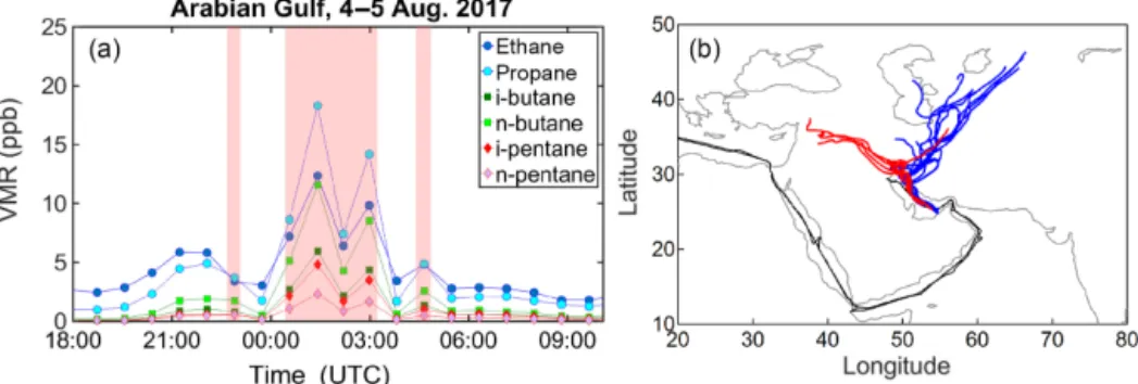
Despite the high correlation between pentane isomers in the AG, several samples and in particular five samples with i-pentane > 1 ppb deviate substantially from the derived slope (Fig. 5), displaying a higher i- / n-pentane ratio. Six-day HYSPLIT back-trajectories show that these particular sam-ples were influenced by the large-scale oil fields (US-CIA, 2007) and gas flaring areas (https://skytruth.org/viirs/, last access: 20 May 2019) in addition to major cities in Iraq (Fig. 7). Before and after encountering the plume of high i-to n-pentane ratios, the back-trajeci-tories extend i-to the gas fields of Turkmenistan before crossing Iran and reaching the sampling point. Apart from the distinctly high i- / n-pentane ratio, the common feature of all samples that originated from the Iraqi oil fields is the high n-butane and propane mixing ratios that reached values of up to 27 and 54 ppb respectively.
3.2.2 Correlation with propane mixing ratios
Elevated propane mixing ratios are usually associated with natural gas processing and petroleum refining. Light alka-nes, such as ethane, n-butane and n-pentane, are co-emitted by O&G activities and, due to their short lifetimes, a tight correlation with propane indicates common sources and little
Figure 5. Relationship between pentane isomers. Linear fits of the data obtained in the Arabian Gulf, Suez Canal, and Jeddah port are compared to enhancement ratio slopes (ERs) from the literature with values for raw and natural gas (aGilman et al., 2013), urban areas (bBaker et al., 2008), gasoline vapours (c Gentner et al., 2009), vehicle emissions (dBroderick and Marnane, 2002), and the Texas ship channel (eBlake et al., 2014). Complete regression statistics: AG: 0.93 × +0.13, R2=0.97; SC: 1.71 × −0.02, R2=0.98; JP: 2.9 × +0.09, R2=0.96; KI ship exhaust: 1.59 × +0.01, R2=0.99.
Figure 6. Composition of a typical KI ship exhaust sample. Aro-matics include benzene (2.8 %), toluene (4.9 %), and m-, p- xylenes (3.1 %), hexanes and higher alkanes include i-hexane (2.6 %), n-hexane (2.7 %), n-heptane (2.2 %), and octane (1.2 %), and other alkanes include trans-2-butene (0.8 %), butene (1.5 %), and 1-pentene (1.2 %). The sample was measured over the Arabian Sea and background ambient mixing ratios were subtracted prior to relative composition calculation. Ethane mixing ratios were 28 ppt lower inside the exhaust sample, being within the uncertainty range of the measurement.
photochemical processing. Therefore, propane is frequently regarded as a sensitive indicator of local/regional emission sources (Helmig et al., 2016).
Weak propane–NMHC correlations were generally ob-served over the MS, RSS, GA, AS, and GO despite occa-sional co-variation related to specific sources. In these areas, propane mixing ratios were relatively low, with median val-ues ranging from 107 ppt over the AS to 355 ppt at the GO (Table 2). The higher mixing ratios that were measured over
the GO are associated with influences by O&G activities in Oman, but the number of samples with elevated propane mix-ing ratios was outnumbered by the samples originatmix-ing from the Arabian Sea. Considering the complete propane dataset, the aforementioned regions displayed only moderate corre-lations with the longer-lived ethane (0.47 < R2<0.72) and poor correlations with the rest of the alkanes, alkenes, and aromatics.
The three regions that showed a high correlation between propane and NMHCs were the SC, RSN, and AG (Fig. 8, Table 3). Among them, the propane–NMHC relationship was markedly different in the SC as propane mixing ra-tios were correlating only with butanes, alkenes, and aro-matic hydrocarbons. N -butane in particular was the only hydrocarbon that was emitted more strongly than propane (ER = 1.1 ppb ppb−1, R2=0.91), while the known tight re-lationship with its isomer i-butane resulted in an enhance-ment mixing ratio slope of 0.43 ppb ppb−1 (R2=0.89) for i-butane. The SC was the only region that had high propane correlations with alkenes (0.73 < R2<0.81) and aromatic hydrocarbons (0.87 < R2<0.91), with ethene and toluene displaying the highest enhancement ratios towards propane, with values of 0.22 and 0.24 ppb ppb−1respectively. The co-emission with combustion tracers, such as aromatic hydro-carbons and the highly reactive alkenes, provide further ev-idence that fresh marine traffic emissions dominate NMHC abundance in this area. Finally, the poor relationship between propane and ethane in the SC is in agreement with our ship exhaust observations, showing that ethane is not emitted by ships.
In contrast to the SC, RSN and AG measurements dis-played high correlation coefficients with ethane that was
Figure 7. Time series of C2–C5alkane volume mixing ratios (a) and back-trajectories (a) of samples collected in the AG on 4–5 August 2017. In (b) the red trajectories correspond to the shaded red data points of (a), while the blue trajectories correspond to all other samples. The back-trajectories start at the ship position and follow the air masses back in time for 6 days on an hourly time grid.
Figure 8. Correlations between propane and selected NMHCs for the areas of the Arabian Gulf (AG, red diamonds), Red Sea North (RSN, green circles) and Suez Canal and Gulf (SC, yellow squares).
found at even higher mixing ratios than propane in the RSN (ER = 1.3 ppb ppb−1, R2=0.95). A similar enhance-ment ratio (1.5 ppb ppb−1) has been reported by Swarthout et al. (2013) from the Boulder Atmospheric Observatory (BAO) within a wind sector representative of natural gas sources. Likewise, butane and pentane isomers showed high correla-tions with propane and with enhancement ratio slopes (Ta-ble 3) that are very similar to those observed in BAO (Pétron et al., 2012, 2014; Gilman et al., 2013; Thompson et al., 2014; Swarthout et al., 2013). Benzene and toluene also cor-related with propane, but with moderate correlation coeffi-cients, as the fit is mainly affected by the larger variability of these species in the southern part of the RSN. Overall, the relationships between propane and the rest of the hydrocar-bons measured provide indications of a natural gas source in the region that is not documented in O&G cartographic maps (US-CIA, 2007). Etiope and Ciccioli (2009) have shown that the RSN has a substantial coverage of geothermal and
vol-canic spots that could potentially explain the high mixing ra-tios of NMHCs measured in this region.
The Arabian Gulf is a global hot-spot for O&G activities. The correlations of alkanes with ambient propane mixing ra-tios were very similar to the ones from the RSN, with the main difference being that ethane was emitted at lower rates (ER = 0.91 ppb ppb−1, R2=0.9) and i-butane at higher rates (ER = 0.52 ppb ppb−1, R2=0.83). Aromatic hydrocarbons did not correlate well with propane in the AG, where the aro-matic hydrocarbon measurements are in the low range due to missing measurements along the northern, more polluted part of the AG (see Figs. S17–S19). Despite the generally high correlation between propane and the rest of the alkanes in the AG, the highest propane mixing ratios ([C3H8] >∼ 10 ppb)
had slightly different interrelationships with all hydrocar-bons, which is attributed to a different air-mass origin (and therefore source), as seen for example in the case study of Fig. 7.
Table 3. Correlation matrix of enhancement volume mixing ratio slopes for selected alkanes and aromatics with propane and methane mixing ratios. Bold values indicate correlations with R2>0.7.
Suez Canal Red Sea North Arabian Gulf
ERVOC/C3H8 R2 ERVOC/CH4 R2 ERVOC/C3H8 R2 ERVOC/CH4 R2 ERVOC/C3H8 R2 ERVOC/CH4 R2
(ppb ppb−1) (ppt ppb−1) (ppb ppb−1) (ppt ppb−1) (ppb ppb−1) (ppt ppb−1) ethane 0.35 0.22 6.8 0.57 1.3 0.95 64 0.67 0.91 0.9 106.5 0.23 propane 18.4 0.71 47.8 0.7 115 0.35 i-butane 0.43 0.89 9.7 0.91 0.22 0.94 11.8 0.75 0.39 0.83 45.1 0.3 n-butane 1.1 0.91 20.1 0.82 0.5 0.96 24.5 0.7 0.52 0.97 63.6 0.38 i-pentane 0.19 0.51 4.9 0.63 0.22 0.91 10.2 0.62 0.18 0.92 21.4 0.34 n-pentane 0.11 0.5 2.5 0.57 0.17 0.91 8 0.59 0.19 0.92 22.8 0.34 benzene 0.1 0.91 1.5 0.83 0.017 0.47 1.1 0.72 0.019 0.3 0.89 0.12 toluene 0.24 0.87 2.4 0.11 0.025 0.59 1.2 0.53 0.0005 0.01 0.29 0.03 xylenes 0.09 0.87 0.9 0.12 0.001 0.01 0.27 0.03 0.0012 0.01 0.1 0.12
Figure 9. Excess mixing ratios of ethane and propane coloured by the excess NMHC mole fraction (EMF) of each sample for the area of the AG. The photo shows the oil slick as seen from the deck during the particular sample.
3.2.3 Excess mole fraction
To further investigate the different interrelationships ob-served under high propane mixing ratios in the AG, and to generally provide a quantitative characterization of hydrocar-bons in each region, their relative abundance was calculated. We define as “excess NMHC mole fraction” (EMF) the rel-ative abundance of non-methane hydrocarbons to the sum of methane and non-methane mixing ratios, whereby the back-ground mixing ratios (defined as the lowest 1 % of regional samples) of each area were subtracted from the total mixing ratios, resulting in the following equation:
Excess NMHC mole fraction (EMF) (1)
= P(NMHC − NMHCBG)
([CH4] − [CH4]BG) +P(NMHC − NMHCBG)
×100 %.
While methane on the global scale is primarily emitted by wetlands, agriculture, and waste sources, natural gas and petroleum systems contribute up to a quarter of global an-thropogenic emission and 10 % of the global source (War-neck and Williams, 2012; Kirschke et al., 2013; Saunois et
al., 2016). Non-associated natural gas (produced by reser-voirs without liquid) composition is dominated by methane, while associated gas contains smaller fractions of methane and higher fractions of alkanes (Farry, 1998; Matar and Hatch, 2001; Anosike et al., 2016). Figure 9 shows the propane versus ethane mixing ratios in the AG, coloured by the excess NMHC mole fraction. Propane and ethane dis-play different relationships under high EMFs, where ethane is higher than propane, with an enhancement ratio slope of 1.1 ppb ppb−1when considering EMF > 20 %. Similar ratios have been obtained through the use of PMF (positive matrix factorization) analysis for oil refineries in Houston (Kim et al., 2005; Buzcu and Fraser, 2006) and with measurements over an oil well (Colombo et al., 2013).
On 29 July 2017 at 12:00 UTC, KI crossed an oil slick in the AG over which a 10 min sample was collected. This par-ticular sample contained 30.1 ppb of C2–C8 hydrocarbons,
consisting mainly of alkanes and aromatics, while the mix-ing ratios of alkenes remained at similar levels to the samples before and after the oil slick. Its excess mole fraction (21 %) and position on the respective linear fit indicate that associ-ated gas contains a larger fraction of NMHCs. The composi-tion of this sample (see Fig. S21) indicates a high fraccomposi-tion of light alkanes, but considering that the most volatile species tend to evaporate first, we cannot establish the representa-tiveness of the actual composition of an oil slick.
Higher EMFs were assigned to back-trajectories origi-nating from the oil fields and refineries of Iran, while the lower EMFs were associated with trajectories originating from the gas fields of Turkmenistan (see notably the case study of Fig. 7). Our analysis supports the notion that as-sociated gas contains more non-methane hydrocarbons than non-associated gas, and that EMF can therefore be used to distinguish between emissions related to oil versus gas ex-ploitation. We find also that the relationship between ethane and propane can be used to identify the type of emission source. Nonetheless, this observation is valid only for rel-atively fresh emissions as the shorter propane lifetime will
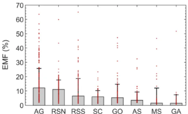
Figure 10. Spatial excess NMHC mole fractions. Bars represent the regional median and error bars the standard deviation. Individual samples are shown with red dots.
modify the ethane-to-propane ratio in chemically processed air masses.
All regions occasionally yielded samples with relatively high EMFs (Fig. 10) that were possibly related to oil slicks or oil production activity sources. A prominent example is the GO. Besides the AG (12 ± 13.7 %), the northern part of Red Sea had, with a median EMF value of 11 ± 6.6 %, the smallest regional standard deviation calculated. This obser-vation is indicative of a widespread and relatively homoge-nous source of NMHCs in the area as the sum of alkanes was on average the second highest encountered along the sam-pled regions. Pentane isomers (Sect. 3.2.1) and relationships with propane (Sect. 3.2.2) indicated that ship emissions dom-inated the NMHC abundance in the SC. The high correlation coefficients between methane and the majority of NMHCs in combination with the poor correlation with ethane in this area (Table 3) confirm that the EMF in the SC is primarily driven by marine traffic, a known source of both methane and non-methane hydrocarbons (Eyring et al., 2005) but with varying relationships depending on the ship type and fuel used (An-derson et al., 2015). The areas of the GA and AS were dom-inated by CH4(EMFs < 5 %) which was frequently close to
global background levels. In the absence of regional emis-sion sources, the more reactive NMHCs are removed by at-mospheric radicals, and the longer-lived methane, which has a large oceanic source (e.g. Bange et al., 1998; Born et al., 2017), dominates the mole fraction. Therefore, these areas are more appropriate for investigation of atmospheric oxida-tion processes than the identificaoxida-tion and characterizaoxida-tion of emissions.
3.3 Sink characterization through NMHCs
3.3.1 Variability–lifetime relationship
The relationship between the variability of atmospheric mix-ing ratios and their chemical lifetimes can be used to evalu-ate the relative importance of chemical reactions and source proximity in the observed variability of trace gases (Junge,
1974; Jobson et al., 1998, 1999; Williams et al., 2000, 2001; Pszenny et al., 2007; Helmig et al., 2008). The conceptual approach has also been extended to particles (Williams et al., 2002). Jobson et al. (1998) introduced the standard deviation of the natural logarithms of the mixing ratios as a useful mea-sure for the variability for short-lived species. The relation-ship with chemical lifetime follows a power-law distribution of the form S (ln (X)) = A × τ−b, (2) where τ = 1 kOH, X[OH] + kCl,X[Cl] + kNO3,X[NO3] . (3)
Here, S is the standard deviation of the natural logarithm of hydrocarbon X with a calculated chemical lifetime (τ ) with respect to reaction with the hydroxyl [OH], chlorine atoms [Cl], and the nitrate [NO3] radicals. A and b are fitting
pa-rameters that are determined by the regression. The term A has been interpreted (although interpretations vary) as re-lated to the standard deviation of the air mass transport times, while b is a robust indicator of the dependence of the mea-sured variability on atmospheric chemistry (as opposed to source proximity) and hence remoteness from sources (Job-son et al., 1998). The relationship has also been exploited in the past to derive gas and particle lifetimes, to determine data quality, and to estimate radical abundances (Williams et al., 2000). In general, higher variability is expected for the most reactive species (Junge, 1974). The parameter b ranges from 0 (indicating close-by sources and no dependence on chem-istry) to around 0.6 (a value that is typical of remote locations in the troposphere).
The chemical lifetime depends on the respective reaction rate coefficients and on the OH, O3, NO3, and Cl
concen-trations. For our calculations we use the average regional radical concentrations as they have been calculated by the EMAC-MOM chemistry model (Table 4), combined with the reaction rates shown in Table 5. We chose to investigate the relationship solely with C2–C5alkanes as these species were
above the detection limit for all areas and therefore provide a robust measure for comparing different regions. They also do not react rapidly with ozone, so this can be neglected. In addition, we found that reactions with the nitrate radical (NO3) are negligible (i.e. do not affect the calculated
life-times; < 1 % changes) due to their low rate coefficients with C2–C5 alkanes (Atkinson, 1991; http://iupac.pole-ether.fr/,
last access: 20 May 2019).
Figure 11 shows that the smallest b value was derived for the AG (0.16±0.09), a region where adjacent O&G activities dominated the emissions, resulting in increased and highly variable alkane mixing ratios (25.44 ± 33.33 ppb). Due to the source proximity, C2–C5hydrocarbon variability was not
significantly related to the chemical reactions. Similarly, the small bRSN(0.22 ± 0.11) is also indicative of nearby sources,
Figure 11. Lifetime–variability relationship for C2–C5alkanes in all regions.
so that wind direction rather than oxidation time determines atmospheric variability. The RSN displayed smaller standard deviations and higher atmospheric lifetimes for all species. Both bAGand bRSN fall in the lowest range of b values that
are consistent with nearby emission sources.
The SC and GO displayed very similar b factors from the variability–lifetime relationships, and were both higher than found in the AG. The highest variability along the route was encountered in the SC, which is also the area with the mod-elled highest OH and Cl concentrations, resulting in shorter lifetimes. Therefore, the bSC(0.33 ± 0.27) represents a
com-bination of regional sources and oxidation processes. Simi-larly, the GO (bGO=0.28 ± 0.23) had high OH but low Cl
concentrations according to the model and mixing ratio vari-ability. In this case the standard deviation of the most reactive pentanes drives the fit. Considering the AS, the poor regres-sion fit (R2=0.33) does not allow interpretation of the de-rived parameters, but it is indicative of local biogenic sources as the variability–lifetime relationship is not as clear as ex-pected for remote sources.
The areas with the highest dependence of variability on chemistry were found to be the GA, MS, and RSS. In these regions, the variability of the measured mixing ratios was more affected by chemistry than the other regions, indicat-ing that these areas are more remote from the sources, and the air had longer chemical processing times indicated by the high b factor (bGA=0.58 ± 0.38, bMS=0.48 ± 0.16,
bRSS=0.41 ± 0.21). Similar values have been reported for
unpolluted coastal sites (0.56 at Nova Scotia, Jobson et al., 1998), marine-influenced air masses (0.54 at Appledore is-land, Pszenny et al., 2007; 0.64 at Surinam, Williams et al., 2000), and the eastern Mediterranean Sea (0.49, Arsene et al., 2007), validating our indications of the importance of alkane–radical reactions in these regions.
3.3.2 Characterization of radical chemistry
The atmospheric ratio of i-butane to n-butane has been fre-quently reported to be between 0.3 and 0.8 for a wide range of environmental conditions (e.g. Baker et al., 2016; Ross-abi and Helmig, 2018). For the AQABA campaign, the iso-meric ratio was on average 0.63±0.44 (median = 0.56), with 82.4 % of the samples between 0.3 and 0.8. The almost iden-tical reaction rate coefficient of the butane isomers (i- and n-) to the OH radical means that their measured ratio will remain relatively constant and equal to the emission ratio in-dependent of transport times, provided only OH reacts with the species and in-mixing is negligible. Deviation from this range would imply a local source with a different emission ratio or oxidation with another radical with which the iso-mers react at different rates. Since the reaction rate coeffi-cient of n-butane is about 40 % faster than i-butane with Cl, these ratios can be used to investigate the presence of Cl rad-icals.
As shown in Fig. 12, three clusters of data substantially deviate from the slope, displaying different i-butane to n-butane mixing ratios. The first cluster (termed case study CS1AG, N = 20; black circles) corresponds to the high
mix-ing ratios encountered in the AG with an isomeric ratio of 1.09 ± 0.18. Considering the small standard deviation of the ratio along with the small geographical coverage, it is more likely that this cluster corresponds to stronger i-butane emissions rather than n-butane depletion due to reaction with Cl radicals. I -butane is more abundant in gas flares (Emam, 2015) which typically contain 45 %–70 % methane (Umukoro and Ismail, 2017). EMF values were on average 35.8 ± 9.5 %, indicating that these particular samples had a very high NMHC content, including the gas-flaring product 1-butene which was 3 times higher compared to the AG av-erage. In addition, these samples cover 15 h, including both day and night times during which Cl concentrations vary substantially. Therefore, Cl reactions are unlikely to be the
Figure 12. (a) Relationship between butane isomers and (b) distribution of the i-butane / n-butane ratio considering all data (grey bars) and the case study data (blue and red bars) as they have been selected from (a).
Table 4. Spatial average OH and Cl concentrations simulated by MOM.
Area [OH] [Cl] [NO3]
(molec. cm−3) (molec. cm−3) (molec. cm−3) MS 2.4 × 10⁶ 6.8 × 10³ 1.1 × 10⁸ SC 5.2 × 10⁶ 1.1 × 10⁴ 3.3 × 10⁸ RSN 4.4 × 10⁶ 1.9 × 10³ 5.3 × 10⁸ RSS 4.5 × 10⁶ 0.5 × 10³ 4.7 × 10⁸ GA 3.3 × 10⁶ 9.9 × 10³ 1.6 × 10⁸ AS 2.3 × 10⁶ 1.3 × 10⁴ 0.9 × 17 GO 5.3 × 10⁶ 1.9 × 10³ 5.2 × 10⁸ AG 4.6 × 10⁶ 2.3 × 10³ 9.8 × 10⁸
main reason for the observed anomalous ratio cluster, and it is more likely that gas-flaring emissions are responsible for this observation. Another example is the cluster of data that belongs to the AS but falls below the commonly observed emission ratio range (CS2AS, N = 43; cyan dots). These are
indicative of oceanic emissions of butanes, which are esti-mated to be emitted at a rate of 0.11 Tg yr−1, exceeded in the alkane series only by ethane (0.54 Tg yr−1) and propane (0.35 Tg yr−1) (Pozzer et al., 2010). Broadgate et al. (1997) reported that n-butane emissions from the North Sea are ∼ 4 times stronger that its isomer, possibly explaining the small ratio (0.34 ± 0.1) we observed in the unpolluted region of the AS. Finally, the third cluster of measurements (CS3, N = 38, blue squares) was mainly made over the Red Sea in the re-gions RSS (N = 15) and RSN (N = 11). In addition, 12 sam-ples from the GO, MS, and SC exhibit a higher i- / n-butane ratio and were clustered together in a group that had an av-erage isomeric ratio of 1.84 ± 1.66. The higher and highly variable isomeric butane ratios, combined with their compar-atively low concentration of both i- and n-butane, suggest Cl-influenced oxidative air masses, but nearby ship emissions could also explain this observation.
In the absence of measurement techniques that could quan-tify Cl radical concentrations directly, the most commonly
Figure 13. Observations of selected VOC tracer ratios (i-butane, n-butane, propane) together with their expected evolution for OH and Cl oxidation from global emission ratios (yellow diamond). The dashed lines indicate the lowest (62 : 1), highest (1.1 × 10⁵:1), and average (930 : 1) OH-to-Cl ratios derived from the EMAC model.
used method to determine whether Cl chemistry has occurred is the examination of VOC ratios and inter-relationships (Jobson et al., 1994; Rudolf et al., 1997; Baker et al., 2016). Figure 13 shows the correlation between an OH-reactive pair (i-butane to propane) and a Cl-reactive pair (i-butane to n-butane). If only OH chemistry acts on the air parcel, the i-butane to n-butane ratio will remain approximately un-changed, while the i-butane to propane ratio will decrease with processing time since the OH+ i-butane rate coefficient is twice that of OH+ propane (Table 5). If only Cl chemistry acts on the air parcel, the opposite is expected: the i-butane to propane ratio will remain unchanged, while the isomeric ra-tio will increase with processing since n-butane reacts faster than its isomer with Cl radicals. Figure 13 shows that the ma-jority of the samples display an unchanged isomeric butane ratio over 2 orders of magnitude of the i-butane to propane ratio, indicating that sources with similar emissions ratios and OH chemistry dominated the air parcels that were
en-Table 5. Reaction rate constants of C2–C5alkanes.
Compound kOH kCL kNO3
(cm3molecule−1s−1) (cm3molecule−1s−1) (cm3molecule−1s−1) ethane 2.5 × 10⁻¹³ 5.9 × 10⁻¹¹ 1.0 × 10⁻¹⁷ propane 1.1 × 10⁻¹³ 1.4 × 10⁻¹⁰ 7.0 × 10⁻¹⁷ i-butane 2.1 × 10⁻¹³ 1.4 × 10⁻¹⁰ 1.1 × 10⁻¹⁶ n-butane 2.3 × 10⁻¹³ 2.2 × 10⁻¹⁰ 4.6 × 10⁻¹⁷ i-pentane 3.6 × 10⁻¹³ 2.2 × 10⁻¹⁰ 1.6 × 10⁻¹⁶ n-pentane 3.8 × 10⁻¹³ 2.8 × 10⁻¹⁰ 8.7 × 10⁻¹⁷
countered along the route. However, a significant portion of the data display isomeric ratios which indicate a mixture of OH and Cl chemical processing.
To evaluate the contribution of OH and Cl radical re-actions in the atmospheric processing, kinetic simulations were used to illustrate the expected tracer ratio evolution (i-butane, n-(i-butane, and propane) starting from average global emission ratios (yellow diamond in Fig. 13, Pozzer et al., 2010). The total OH radical concentration was held at 5 × 10⁶molec. cm−3and the OH / Cl ratios were adjusted to sim-ulate conditions that range between OH reactions only and Cl reactions only. In order to demonstrate plausible atmo-spheric ranges for the OH / Cl ratio, the lowest (62 : 1), high-est (1.1 × 10⁶:1), and average (930 : 1) ratios were gener-ated in the EMAC model run for the campaign, and these have been implemented in Fig. 13. In the model the Cl rad-ical is generated from HCl oxidation, the former being re-leased from sea spray via acid displacement (Erickson et al., 1999; Keene et al., 1999; Knipping et al., 2000; Young et al., 2014). Modelled Cl concentrations are therefore expected to be more abundant over the marine boundary layer and coastal areas. In the atmosphere, ClNO2represents a further form of
reactive chlorine, which is formed in heterogeneous reactions of N2O5with sea salt at night-time and which has been
de-tected at significant concentrations in both coastal and conti-nental air masses (Thornton et al. 2010; Phillips et al., 2012). ClNO2can photolyse to produce Cl radicals (Osthoff et al.,
2008; Lawler et al., 2009; Riedel et al., 2012; Young et al., 2012) and field observations have shown that ClNO2can be
responsible for more than 50 % of near-surface Cl produc-tion during early morning (Young et al., 2012; Mielke et al., 2013; Young et al., 2014). As the EMAC model does not in-clude the formation of ClNO2, we may assume that ambient
OH / Cl ratios may in fact be lower than the minimum 62 : 1 ratio generated by the model.
Based on the kinetic model results, the OH / Cl ratio can be expressed as a function of the slope (σ ) of the tracer ratio evolution of these particular hydrocarbons as
OH Cl =
−80
σ +0.2, (4)
where σ corresponds to the slope of ln(i-butane / propane) to ln(i-butane / n-butane) with evolution times illustrated in the colour scale of Fig. 13. Equation (4) is independent of the initial emission ratios and of the absolute radical con-centrations, but it is sensitive to reaction rate coefficients. Therefore, it is only applicable in this form in this region, assuming that the reaction rate coefficients that are presented in Table 5 are applicable. A more general expression for the relationship of the rate coefficients and OH / Cl ratio under large temperature variations (e.g. free troposphere) was pre-sented in Rudolf et al. (1997).
Figure 13 shows that some data points lie on positive slopes which define the unrealistic case in which Cl radicals were the only oxidant acting on the hydrocarbons. This in-cludes the clusters of points discussed previously (CS1 and CS3), reaffirming that they are unusual emission signatures rather than the result of Cl radical chemistry. It is interest-ing to note that many of the points in this part of the graph have been affected by our own ship exhaust. Therefore our own ship and possibly other vessels emit propane, i-butane, and n-butane in ratios that are distinctly different from those generated from any combination of OH and Cl radical chem-istry acting on the gases when emitted at the average emis-sion ratio (see the yellow marker in Fig. 13). Nonetheless, the majority of the samples collected over the RSN and over the AG lie on trend lines that match the theoretical slope of an OH / Cl ratio of ≈ 200 : 1. As an example, Fig. 13 illus-trates the regression statistics for the majority of the sam-ples collected in the RSN (green line, σ = −0.63). Utiliz-ing Eq. (4), the resultUtiliz-ing radical ratio is 186 : 1. Our analysis demonstrates that oxidative pairs can be used to provide an indication of the presence of Cl atoms and provide a rough estimate of atmospheric OH-to-Cl ratios.
4 Summary and conclusions
An overview of the atmospheric mixing ratios measured around the Arabian Peninsula during the AQABA ship cam-paign was provided in terms of regional abundance. The highest mixing ratios were observed over the Arabian Gulf, the Suez Canal, and the northern parts of the Red Sea, and