HAL Id: hal-01395058
https://hal.sorbonne-universite.fr/hal-01395058
Submitted on 10 Nov 2016
HAL is a multi-disciplinary open access archive for the deposit and dissemination of sci-entific research documents, whether they are pub-lished or not. The documents may come from teaching and research institutions in France or abroad, or from public or private research centers.
L’archive ouverte pluridisciplinaire HAL, est destinée au dépôt et à la diffusion de documents scientifiques de niveau recherche, publiés ou non, émanant des établissements d’enseignement et de recherche français ou étrangers, des laboratoires publics ou privés.
Multichannel processing for dispersion curves extraction
of ultrasonic axial-transmission signals: Comparisons
and case studies
Kailiang Xu, Dean Ta, Didier Cassereau, Bo Hu, Weiqi Wang, Pascal Laugier,
Jean-Gabriel Minonzio
To cite this version:
Kailiang Xu, Dean Ta, Didier Cassereau, Bo Hu, Weiqi Wang, et al.. Multichannel processing for dispersion curves extraction of ultrasonic axial-transmission signals: Comparisons and case studies. Journal of the Acoustical Society of America, Acoustical Society of America, 2016, 140 (3), pp.1758 -1770. �10.1121/1.4962491�. �hal-01395058�
Multichannel Processing for Dispersion Curves Extraction of Ultrasonic Axial-Transmission 1
Signals: Comparisons and Case Studies 2
3
1. Kailiang Xu
4
Department of Electronic Engineering Fudan University, Handan Road No 220, 200433, Shanghai, China.
5
Sorbonne Universités, UPMC Univ Paris 06, CNRS, INSERM, Laboratoire d’Imagerie Biomédicale
6
(LIB), 15 rue de l'école de médecine, 75006, Paris, France
7
2. Dean Ta
8
Department of Electronic Engineering Fudan University, Handan Road No 220, 200433, Shanghai, China.
9
State Key Laboratory of ASIC and System, Fudan University, Shanghai, China;
10
Key Laboratory of Medical Imaging Computing and Computer Assisted Intervention (MICCAI) of
11
Shanghai, Shanghai, China.
12
3. Didier Cassereau
13
Sorbonne Universités, UPMC Univ Paris 06, CNRS, INSERM, Laboratoire d’Imagerie Biomédicale
14
(LIB), 15 rue de l'école de médecine, 75006, Paris, France
15
4. Bo Hu
16
Department of Electronic Engineering Fudan University, Handan Road No 220, 200433, Shanghai, China.
17
5. Weiqi Wang
18
Department of Electronic Engineering Fudan University, Handan Road No 220, 200433, Shanghai, China.
19
6. Pascal Laugier
20
Sorbonne Universités, UPMC Univ Paris 06, CNRS, INSERM, Laboratoire d’Imagerie Biomédicale
21
(LIB), 15 rue de l'école de médecine, 75006, Paris, France
22
7. Jean-Gabriel Minonzio
23
Sorbonne Universités, UPMC Univ Paris 06, CNRS, INSERM, Laboratoire d’Imagerie Biomédicale
24
(LIB), 15 rue de l'école de médecine, 75006, Paris, France
25 26
Abstract — Some pioneering studies have shown the clinical feasibility of long bones evaluation using
1
ultrasonic guided waves. Such a strategy is typically designed to determine the dispersion information of
2
the guided modes to infer the elastic and structural characteristics of cortical bone. However, there are still
3
some challenges to extract multimode dispersion curves due to many practical limitations, e.g., high
4
spectral density of modes, limited spectral resolution and poor signal-to-noise ratio (SNR). Recently, two
5
representative signal processing methods have been proposed to improve the dispersion curves extraction.
6
The first method is based on singular value decomposition (SVD) with advantages of multi-emitter and
7
multi-receiver configuration for enhanced mode extraction; the second one uses linear Radon transform
8
(LRT) with high-resolution imaging of the dispersion curves. To clarify the pros and cons, a face to face
9
comparison was performed between the two methods. The results suggest that the LRT method is suitable
10
to separate the guided modes at low frequency-thickness-product (𝒇 ∙ 𝒉) range; for multimode signals in
11
broadband 𝒇 ∙ 𝒉 range, the SVD-based method shows more robust performances for weak mode
12
enhancement and noise filtering. Different methods are valuable to cover the entire 𝒇 ∙ 𝒉 range for
13
processing ultrasonic axial transmission signals measured in long cortical bones.
14 15
Keywords: Waveguides; Singular value decomposition; Linear Radon transform; Dispersion curves 16
PACS: 43.60.Fg, 43.60.Gk, 43.80.Vj, 43.80.Jz, 43.80.Ev 17
1
I. INTRODUCTION
2
In the past decade, significant progress has been achieved in quantitative ultrasound (QUS) assessment
3
of cortical bone using axial transmission techniques 1,2. Such techniques are intended to osteoporotic
4
fracture discrimination 3 or to fracture healing monitoring 4,5. Several axial transmission techniques have 5
been explored using either one transmitter/one receiver 6, one transmitter/multiple-receiver 7, or
6
multiple-transmitter/multiple-receiver configurations 8. Signal analysis developed for clinical applications
7
are based on velocity measurement of a single signal, such as the first arriving signal (FAS) 6, or a slower 8
second energetic wave which has been interpreted as the fundamental anti-symmetrical A0 Lamb mode
9
based on plate model 7. If the cortical thickness is much smaller than the longitudinal wavelength, FAS can
10
be seen as the S0 Lamb mode. If the cortical thickness is much larger than the longitudinal wavelength, the
11
FAS corresponds to the non-dispersive lateral compression wave 7. In between, when the thickness is
12
comparable to the wavelength (e.g., at 1 MHz, the wavelength in cortical bone is 3 to 4 mm), a physical
13
interpretation of the FAS has yet to be provided. Besides FAS, reflection and conversion of ultrasonic body
14
waves have been observed in the relatively thick bovine tibia ex vivo 9. 15
Whereas the signal analysis techniques applied so far in axial transmission meet the need for simplicity
16
and pragmatism, the corresponding biomarkers extracted from a single signal (either FAS or A0 mode)
17
provide an incomplete biomechanical characterization of bone strength. Such a consideration has
18
motivated the research aiming at fully characterizing the response of cortical long bones to an ultrasonic
19
excitation. Particularly, considering that long bones actually support the propagation of multiple guided
20
modes, several studies have shown interest in measuring and interpreting the dispersion curves of guided
21
waves within a wideband frequency-wavenumber range 1,2. Measurement of dispersion curves, along with
22
suitable waveguide modeling, has been proposed for concurrent estimation of cortical thickness and elastic
23
properties 10-14. However, the extraction and accurate interpretation of the dispersion characteristics of
24
guided modes propagating along the cortical shell of long bones pose difficulties, such as the high spectral
25
density of modes, limited spectral resolution and poor signal-to-noise ratio (SNR).
26
Particularly, because of the limited spatial sampling or resolution achievable in clinical measurements
27
with clinical probes (typically a few cm-long array), the traditional two-dimensional (or spatio-temporal)
28
Fourier transform (2D-FT) 15 cannot achieve a high wavenumber resolution for complete multimode
29
separation 2. From guided signal processing point of view, several methods have been described to
30
distinguish overlapped modes and to extract the corresponding dispersion curves. These include
31
dispersion-based short-time Fourier transform 16, group velocity filtering 17, time-frequency representation 32
18, warped frequency transform 19, time-frequency ridge extraction 20,21, dispersion compensation 22, blind 33
identification 13, generalized warblet transform 23, adaptive Chirplet transform 24, orthogonality
34
relation-based method 25 and compressed sensing method 26. Recently, two methods taking advantage of a 35
multiple-transmitter/multiple-receiver implementation of axial transmission have been proposed, singular
36
vector decomposition (SVD) 8,27 and linear Radon transform (LRT) 28,29.
37
The SVD-based approach is able to significantly enhance the weak-amplitude modes by selecting the
38
singular values and singular vectors corresponding to the signals and by filtering out the small singular
39
values corresponding to the noise 8. This method, applied in vitro on radius specimens 14 and in vivo at the
40
forearm10, has shown a good performance to estimate cortical thickness. The LRT method is widely known 41
in seismic data processing 30,31. Taking advantage of the sparse inversion, the LRT methods are capable of
42
achieving an energy focusing or so-called high-resolution dispersive energy imaging of the wave-packets
43
whose arrival times are linearly dependent on the propagation path 32,33. The LRT methods have already
44
been applied to study the surface-wave data for Rayleigh wave dispersive energy imaging 34. Recently, the
45
high-resolution LRT method has been introduced to analyze the ultrasonic guided signals in long bone, and
was observed to provide enhanced resolution of theextracted dispersion curves in comparison to the 2D-FT
1
method 28,29.
2
While results on bone have been reported with SVD-based and LRT approach by different groups, the
3
pros and cons as well as the applicability conditions of the two different signal processing techniques have
4
not been thoroughly discussed. In this study, a face to face comparison is performed using SVD-based,
5
LRT and the classical 2D-FT method. Synthetic and experimental signals on bone-mimicking phantoms
6
and on ex-vivo human radius are analyzed.
7
II. BRIEF REVIEW OF THE PROPOSED SIGNAL PROCESSING METHODS 8
Typically, the frequencies used for the axial transmission measurement of long cortical bone are in the
9
range between 50 kHz and 2 MHz and the typical cortical thickness of human radius and tibia are in the
10
range between 1 to 6 mm approximately. According to the characteristics of the guided signals observed in
11
different ranges of the frequency-thickness product (𝑓 ∙ ℎ), three representatives cases can be distinguished,
12
as shown in Table 1: (1) low frequency-thickness product 𝑓 ∙ ℎ < 1 MHz·mm, corresponding to thin
13
cortical bone about 1 mm to 4 mm (mainly for radius), where mainly two fundamental Lamb modes S0 and
14
A0 are observed, (2) intermediate 𝑓 ∙ ℎ range (1 <𝑓 ∙ ℎ<6 MHz·mm) where multiple guided modes overlap
15
without temporally separated wave-packets, and (3) high 𝑓 ∙ ℎ > 6 MHz·mm, corresponding to the thick
16
cortical bone, e.g., tibia, which is mainly in the range of body waves propagation.
17
Various signal processing techniques have been reported to identify and disentangle the overlapping
18
modes for short axial propagation distances. Table II lists the different signal processing approaches
19
proposed for axial transmission, together with a brief description of the methods and conditions of
20
application.
21
III. THEORY AND METHODS 22
A. Guided Waves Dispersion
23
Lamb modes in plates are classified as symmetric (S) and antisymmetric (A) modes, briefly named as
24
𝑆𝑛 and 𝐴𝑛 modes (𝑛 = 0,1, 2, … ), which are solutions of the Rayleigh-Lamb equations 35,36. The 25
dispersion curves can be expressed as wavenumber 𝑘 versus 𝑓 or 𝑓 ∙ ℎ.
26
The 2D-FT provides a general relationship between the distance-time space (𝑥, 𝑡) and
27 frequency-wavenumber space (𝑓, 𝑘). 28 𝑆(𝑘, 𝑓) = ∬ 𝑔(𝑥, 𝑡)𝑒𝑗(𝑘𝑥−2𝜋𝑓𝑡)𝑑𝑥𝑑𝑡. (1), +∞ −∞ 29
where 𝑔(𝑥, 𝑡 ) is the temporal signals recorded at a series of space positions x. The dispersion curves can
30
thus be obtained by locating the wavenumbers at each frequency where the amplitude of 2D-FT result
31
𝑆(𝑘, 𝑓) reaches the maxima.
32
With a given dispersion curve and an excitation signal, spectrum of the dispersive signal at distance 𝑥0
33
can be computed by multiplying a phase-spectrum adjustment term 𝑒−𝑗𝑘(𝑓) 𝑥0 to the spectrum of excitation.
34
The temporal waveforms can thus be obtained by using inverse Fourier transform to the phase-adjusted
35
spectrum of excitation. Such a procedure provides us an efficient way to synthesize the temporal signal
36
𝑔(𝑥, 𝑡) 22. 37
B. Singular Value Decomposition-based Wavenumber Extraction
38
The 3D multi-emitter and multi-receiver signals matrix is denoted as 𝑀(𝐸, 𝑥, 𝑡), where 𝑥 is the distance
39
sampled by 𝑁𝑟 receivers, and 𝐸 denotes different emitters, 𝐸 = 1, 2, … , 𝑁𝑒. ℳ(𝐸, 𝑥, 𝑓) is the spectrum of
40
𝑀(𝐸, 𝑥, 𝑡) in frequency domain. After the SVD decomposition of the 2D response matrix ℳ(𝐸, 𝑥, 𝑓 = 𝑓0)
at each frequency 𝑓0, we obtain two unitary matrices, i.e., an 𝑁𝑒× 𝑁𝑒 matrix 𝑈 and an 𝑁𝑟× 𝑁𝑟 matrix 𝑉,
1
and an 𝑁𝑒× 𝑁𝑟 rectangular matrix ∑ with the singular values as the diagonal entries 𝜎𝑖 (𝑖 = 1, … , 𝑁𝑒).
2
The 𝑁𝑟 columns of 𝑉, i.e., 𝑣𝑖 (𝑖 = 1, … , 𝑁𝑟), are the reception singular vectors. At a particular frequency,
3
only the first 𝑁𝑟𝑘 singular vectors 𝑣𝑖 associated with the most energetic singular values 𝜎𝑖 (𝑖 = 1, … , 𝑁𝑟𝑘)
4
are retained as a basis of the received signal subspace. The wavenumber determination is then achieved by
5
projecting a testing vector onto this basis.
6
The testing vector is expressed as an attenuated spatial plane wave with a complex wavenumber 𝑘 + 𝑗𝛼
7 27 8 𝑣𝑡𝑒𝑠𝑡(𝑘, 𝛼) = 1 √ 𝑁𝑟 2𝛼𝐿 (1 − 𝑒−2𝛼𝐿) 𝑒−𝑗𝑘𝑥−𝛼𝑥 (2a), 9
Denominator term √2𝛼𝐿𝑁𝑟 (1 − 𝑒−2𝛼𝐿) is used to normalize 𝑣𝑡𝑒𝑠𝑡(𝑘, 𝛼)27. 𝛼 is the attenuation coefficient
10
and in the study, a constant was adopted, i.e., 𝛼 = 0.05 𝑁𝑝 ∙ 𝑚𝑚−1. Such a value is close to the average
11
attenuation coefficients of the low-order guided modes in the bone mimicking materials 27. With a constant
12
attenuation coefficient, 𝑣𝑡𝑒𝑠𝑡(𝑘, 𝛼) is a function of 𝑘.
13
At each frequency (𝑘0, 𝑓0), the projection of 𝑣𝑡𝑒𝑠𝑡 onto the 𝑁
𝑟𝑘 first reception singular vector basis
14
𝑣𝑖 (𝑖 = 1, … , 𝑁𝑟𝑘) yields the so-called Norm function 𝑆SVD(𝑘, 𝑓) 8 15 𝑆𝑆𝑉𝐷(𝑘0, 𝑓0) = ∑ |⟨𝑣𝑡𝑒𝑠𝑡(𝑘0, 𝛼)| 𝑣𝑖(𝑓0)⟩|2 𝑁𝑟𝑘(𝑓0) 𝑖=1 (2b), 16 where ⟨𝑣𝑡𝑒𝑠𝑡(𝑘
0, 𝛼)| 𝑣𝑖(𝑓0)⟩ is the Hermitian scalar product between the 𝑣𝑡𝑒𝑠𝑡(𝑘0, 𝛼) and 𝑣𝑖(𝑓0). Thus, at
17
each frequency 𝑓0, the Norm function is a function of 𝑘 and the maxima correspond to wavenumbers of the
18
guided waves presented in the received signals.
19
Due to the normalized characteristics of the orthogonal basis, the values of Norm function range from 0
20
to 1. This value can be interpreted as follows: if a guided mode exists in the signal, the corresponding Norm
21
function value is close to 1; otherwise, the value is close to 0 8. Details of the SVD-based method and
22
corresponding examples can be learned from 8,37. Note that the method can be adapted to achieve a more
23
accurate dispersion extraction when the cortical thickness is not uniform but with linear changes in the
24
direction of wave propagation 38.
25
C. Linear Radon Transformation based Wavenumber Extraction
26
For convenience of the inversion problem, the LRT is usually formulated as the forward relationship
27
between the (𝑥, 𝑡) and the Radon domain. Let 𝑔(𝑥, 𝑡) represent a distance-time matrix measured by single
28
emitter and 𝑁𝑟 receivers. The LRT can be defined using the following equation 30,31
29
𝑔(𝑥, 𝑡) = ∫ 𝑤(𝑝, 𝜏 = 𝑡 − 𝑝𝑥)𝑑𝑝
𝑝
(3),
30
where 𝜏 and 𝑝 denote the intercept time and slope parameter or phase slowness, respectively; 𝑤(𝑝, 𝜏 =
31
𝑡﹣𝑝𝑥) designates the signal in the (𝜏, 𝑝) domain. The LRT is commonly named as 𝜏‐ 𝑝 transform or slant
32
stack.
33
Equation (3) can be rewritten in frequency domain as 28,31
𝐺(𝑥, 𝑓) = ∫ 𝑊(𝑝, 𝑓)𝑒−𝑗2𝜋𝑓𝑝𝑥𝑑𝑝 𝑝
(4).
1
Using matrix notation, we have
2
𝐺 = 𝐿𝑊 (5),
3
The 𝑁𝑟× 𝑁𝑝 linear operator 𝐿 is
4 𝐿 = [𝑒 −𝑗2𝜋𝑓𝑝1𝑥1 … 𝑒−𝑗2𝜋𝑓𝑝𝑁𝑝𝑥1 ⋮ ⋱ ⋮ 𝑒−𝑗2𝜋𝑓𝑝1𝑥𝑁𝑟 … 𝑒−𝑗2𝜋𝑓𝑝𝑁𝑝𝑥𝑁𝑟 ] 𝑝 = 𝑝1, 𝑝2, … , 𝑝𝑁𝑝 (6), 5
where 𝑁𝑝 is the number of the slowness sampling points.
6
A penalized least-squares (LS) solution to Eq. (5) has been introduced by minimizing the following cost
7
function 31,32
8
𝐽 = ‖𝐺 − 𝐿𝑊‖22 + 𝜇𝑄(𝑊) (7),
9
where the Lagrange multiplier 𝜇, also referred as regularization hyperpameter 39, determines the trade-off 10
between the misfit term ‖𝐺 − 𝐿𝑊‖22 describing the data fidelity and the penalty term 𝑄(𝑊) in Radon
11
domain.
12
A typical implementation of the penalty term is to use the quadratic 𝑙2-norm, i.e., 𝑄(𝑊) = ‖𝑊‖22. So
13
that, the LS solution can be analytically obtained as
14
𝑊̃ = (𝐿𝐻𝐿 + 𝜇𝐼)−1𝐿𝐻𝐺 (8).
15
where 𝐿𝐻 is the complex-conjugate transpose of 𝐿. It should be noticed that 𝐿𝐻𝐿 is not a unitary matrix.
16
The 𝑊(𝑝, 𝑓) in the Radon field can be readily mapped to the (𝑘, 𝑓) domain via 𝑘 = 2𝜋𝑓𝑝 28. The
17
dispersion curves can also be obtained from |𝑆𝐿𝑅𝑇(𝑘, 𝑓) |2 by using LRT method.
18
If certain non-quadratic terms, which enable to quantify the amount of sparsity of a vector, are adopted
19
as the penalty terms, then we can focus the signal energy on the “best” subspace of the solution spaces. That
20
is actually the sparse solution leading to the high-resolution LRT method. Therefore, the penalty term
21
actually controls the high resolution constraints and also indicates the sparsity of the results. Two typical
22
non-quadratic penalty terms, i.e., 𝑙1-norm 𝑄(𝑊) = ‖𝑊‖1 and Cauchy norm, are usually adopted for
23
achieving sparsity. The Cauchy norm penalty term is defined as 33
24
𝑄(𝑊) = ∑ 𝑙𝑛[1 + 𝑊(𝑝𝑖, 𝑓)/𝜀2] (9). 𝑁𝑝
𝑖=1
25
where the scale factor of the Cauchy distribution 𝜀2 actually indicates the default power in absence of
26
hyperbolic events33. According to the discrepancy principle, a proper 𝜀2 value should be selected to ensure
27
that the misfit matches the power of noise 40. The one-dimension Brent parabolic interpolation method has 28
been used to compute the epsilon 40,41. It is fixed as a constant 𝜀 = 0.8 in 29. In the study, 𝜀 = 1 was used
29
for the Cauchy LRT computation. Although there is no analytical solution to high-resolution LRT, it can be
30
solved efficiently by conjugate gradient technique. Details of that can be found in literature 39,40.
31
The trade-off curve, so-called L-curve 42, is usually applied for empirical optimization of the 𝜇 value for 32
the penalized LS-LRT and high-resolution LRT method. A small hyperparameter 𝜇 value leads to a
33
solution with minimized misfit term but with less energy focusing; conversely, a larger 𝜇 value can achieve
34
a high resolution by emphasizing the regularization term. For simplicity and methodology comparison, a
fixed value of trade-off 𝜇 = 0.05 were used for the results presented in Section IV. Detailed discussion of
1
trade-off parameter using L-curve can be found in Section V(1).
2
D. Experiments
3
Experiments are achieved using an array transducer consisting in 5 emitters and 24 receivers (Vermon,
4
Tours, France) associated with a specific driving electronic device (Althaïs, Tours, France). The pitch of
5
the array transducer is 0.8 mm and the length and width of each rectangular element are 0.8 mm and 8 mm,
6
respectively. The central frequency is 1 MHz and the ‐6 dB bandwidth goes from 0.5 to 1.6 MHz10.
7
For case II in Table I, experiments are carried out in two phantoms, i.e., a 4 mm-thick bone-mimicking
8
material (Sawbones, Pacific Research Laboratory Inc, Vashon, WA) and 2.5 mm-thick ex-vivo human
9
radius. A 25.5 mm-thick polymethylacrylate (PMMA) plate is also measured for case III in Table 1.
10
Ultrasound gel (Aquasonic, Parker Labs, Inc, Fairfield, NJ) is used to ensure the coupling between the
11
probe and the sample. The characteristics of the specimens are listed in table III. 𝑉𝑇 is the shear velocity,
12
and 𝑉𝐿‖, and 𝑉𝐿⊥ are the pure compression bulk wave velocities in the direction parallel and normal to the
13
direction of the fibers (bone-mimicking material) or to the long axis of the bone (human radius). The
14
density and thickness are denoted by ρ and h. Typical values for human radius density, shear and
15
longitudinal velocity, derived from the literature, are used for computation of the theoretical dispersion
16
curves of the 2D transverse isotropic free plate model 14. The average thickness of the human radius
17
specimen was obtained by X-ray computed tomography (XtremCT, Scanco Medical, Bruttisellen,
18
Switzerland).
19
IV. RESULTS 20
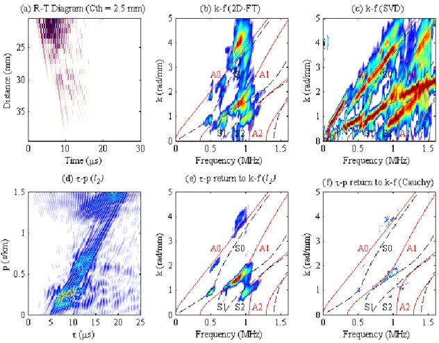
A. Synthetic signals, narrow wavenumber-band Lamb modes S0 and A0
21
This example corresponds to case I in Table I. Two fundamental narrow k-band (0 < 𝑘 ≤ 2 𝑟𝑎𝑑 ∙
22
𝑚𝑚−1) Lamb modes A0 and S0 on a 2 mm-thick bone-mimicking plate were synthesized with
23
peak-to-peak amplitudes of 1 and 0.3, respectively (see Fig. 1a). A Gaussian random noise was added with
24
SNR of 30dB. The SNR is defined as the ratio of the power of the signal and that of the noise. Fig. 1b
25
presents the 2D-FT results in the (𝑘, 𝑓) domain. After SVD decomposition, the singular values were
26
normalized in dB scale. Those singular vectors associated with singular values above the threshold 21dB
27
were remained as the signal subspaces and the rest were filtered out as noise (see Fig. 7a ). The SVD result
28
is depicted in Fig. 1c. Fig. 1d is the (𝜏, 𝑝) result obtained by LRT with 𝑙2-norm. Since there is a large
29
velocity difference between the S0 and A0 modes (see Fig. 1a), they are projected as two separate regions
30
in the (𝜏, 𝑝) domain (Fig. 1d). As shown in Figs. 1e-f, the high-resolution LRT results using 𝑙1-norm and
31
Cauchy norm are able to significantly concentrate the 𝑘﹣𝑓 energy of the narrow wavenumber-band and
32
S0 and A0 modes. The colors of the 𝑘﹣𝑓 and 𝜏﹣𝑝 energy distribution present the mode energy with
33
highest values in red and lowest values in blue.
34
B. Phantom signals
35
(1) Wide wavenumber-band and multiple guided modes
36
This example corresponds to case II in Table I. Figure 2 presents the experimental signals measured in a
37
4 mm-thick bone-mimicking plate. Fig. 2a is the distance-time diagram of the array-signal. As shown by
38
the 2D-FT and SVD 𝑘﹣𝑓 results (Figs. 2b-c), the detectable wavenumber dispersion is in the range of 0 <
39
𝑘 < 4 𝑟𝑎𝑑 ∙ 𝑚𝑚−1 with more than 5 modes. The experimental SNR is around 60dB. Those singular
40
vectors associated with singular values higher than an heuristic threshold of 20dB were remained as the
41
signal subspaces and the rest were filtered out as noise. Fig. 2d plots the 𝑙2-norm-based energy distributions
42
in the (𝜏, 𝑝) domain. Figs 2e-f depict the high-resolution LRT results of the multimode energy distribution
43
in 𝑘﹣𝑓 field using 𝑙1-norm and the Cauchy norm.
Compared with the 2D-FT method, using the SVD-based method, the multimode dispersion curves can
1
be identified with an enhancement of the weak modes, e.g., A0, A1, S0, S4 etc., and also the low-amplitude
2
S0 and A1 mode energy in wavenumber range of 3 < 𝑘 < 4 𝑟𝑎𝑑∙𝑚𝑚−1. In Fig. 2d, the LRT method can
3
obtain a projection in the (𝜏, 𝑝) domain with focused energy points. But as shown in Figs. 2e-f, the
4
concentrated region in the (𝜏, 𝑝) domain only represents the strong modal energy close to the center
5
frequency, which actually cannot lead to an effective reconstruction of the dispersion trajectories of the
6
weak modes. For example, the A0, A1 and S4 modes, whose energy is far from the center frequency of the
7
probe, are not clearly depicted on the LRT results.
8
(2) Body waves
9
This example corresponds to case III in Table I. A 25.5 mm-thick PMMA plate was measured to obtain
10
the signals mainly consisting of ultrasonic body waves. The experimental SNR is as the previous example
11
around 60dB. As ultrasonic body waves have been investigated in a 6.5 mm-thick bovine bone ex vivo 9, 12
such a very-thick plate is also prepared to clarify the performance of the two methods in the high 𝑓 ∙ ℎ
13
range. It should be noted that 25.5 mm-thick waveguides are unlikely to be encountered in human cortical
14
bone whose thickness varies from less than a millimeter to a few millimeters at best.
15
Different from the highly dispersive guided modes in the thin plates (Table I, case II), in a thick plate,
16
there mainly exist body waves propagating as temporally separated wave-packets. As shown in Fig. 3a,
17
there are five different wave-fronts in the distance-time diagram with different ray paths. Pd and Sd
18
represent the longitudinal and shear waves axially propagating along the plate surface. PrP and SrS
19
correspond to the first reflection of the longitudinal and shear waves on the bottom wall. PrS corresponds to
20
the longitudinal-to-shear wave conversion when the P wave is reflected on the bottom surface of the plate.
21
The markers on Fig. 3a were computed according to the distance-velocity relationship. Figs. 3b-c are the
22
2D-FT and SVD 𝑘﹣𝑓 results, respectively. After projecting the array-signal from distance-time domain to
23
Radon field, accurate slowness and amplitude of each wave-packet can be obtained from those energy
24
focusing maxima in τ-p domain, which is convenient for detecting the components with different ray paths.
25
Furthermore, such a slant-stack operator is very suitable to detect the weak components (see Fig. 3d).
26
However, as shown in Figs. 3e-f, for the signals measured in high 𝑓 ∙ ℎ range, there is still no evidence that
27
the 𝑙1-norm and Cauchy norm LRT method can improve the k-f resolution for better dispersive energy
28
imaging. The SVD-based method still provides a result with best dispersion energy extraction in 𝑘﹣𝑓
29
domain.
30
C. Ex vivo guided signals analysis in a human radius
31
This example corresponds to case II in Table I. The guided signals measured from an ex-vivo 2.5
32
mm-thick human radius can be seen in Fig. 4a. Figs. 4b-c are the 2D-FT and SVD 𝑘﹣𝑓 results,
33
respectively. Fig. 4d is the multimode energy distributions in the (𝜏, 𝑝) domain using the 𝑙2-norm LRT
34
method. The experimental SNR is around 55dB (see Fig. 7b). The threshold of singular values is 20dB.
35
Figs. 4e-f show the 𝑘﹣𝑓 energy distribution obtained by 𝑙1-norm and Cauchy norm high-resolution LRT
36
methods. Comparing with the LRT and 2D-FT method, SVD-based method is capable of detecting the
37
noise polluted A0 and S0 mode and also part of A1, A2, S1 and S2 modes in wideband frequency-thickness
38
range. Similar to the 4 mm-thick phantom signals (Fig. 2), because of high dispersive characteristics, the
39
wideband guided modes in the human radius cannot be readily separated and enhanced in the Radon field.
40
The resolution improvement of the fundamental A1, S1 and S2 modes can be observed close to center
41
frequency bandwidth in Fig. 4e using the 𝑙1-norm LRT method, but for the relatively weak and wideband
42
modes, e.g., A0, A2 and S0, the LRT cannot provide sufficient mode enhancement. As shown in Fig. 4f,
43
due to the improper value of the regularization parameter, it seems that the Cauchy norm LRT method
44
enforces the results with “all-zero” solution. The reason of that will be discussed in Section V.
45
V. DISCUSSION 1
In this study, we performed a face to face comparison between two signal processing approaches,
2
namely the SVD-based and LRT method, which have been recently proposed to extract the dispersion
3
curves of guided waves transmitted in long bone. To this goal, the methods were applied to synthetic
4
signals and experimental signals recorded on a bone-mimicking plate and on a human radius ex vivo.
5
A. Parameter optimization of the LRT and SVD-based method
6
The hyperparameter 𝜇 of the LRT methods, which controls the trade-off between data fidelity and mode
7
energy concentration (or sparseness), can be heuristically determined by the L-curve. The optimal value of
8
hyperparameter, usually determined on the “elbow” of L-curves, actually corresponds to the maximal
9
curvature point where the misfit and penalty terms are minimized together 28,42. For the SVD-based method,
10
a SNR threshold is used to selectively separate the noise and signal spaces.
11
(1) Hyperparameter μ of the LRT method
12
It has been observed in Section IV that for case I in Table 1, the LRT methods provide similar 𝑘﹣𝑓
13
dispersion loci as 2D-FT method; but for cases II and III, the over-sparse solutions of k-f energy
14
distributions are readily to be obtained when using the high-resolution LRT methods. To clarify the reason
15
of that, the L-curves are investigated for case I: synthetic signals of narrow wavenumber-band Lamb modes
16
A0 and S0 on a 2 mm-thick phantom plate (Fig. 5) and for case II: 2.5 mm-thick human bone ex vivo (Fig.
17
6). Strictly speaking, the hyperparameter μ needs to be optimized as a function of f, slowness, penalty term
18
and misfit term. Therefore, different L-curves at different frequencies are shown at 3D space of μ, penalty
19
term and misfit term. The optimal values of μ parameter are searched from 2−15 to 27 in different
20
bandwidths of the interest.
21
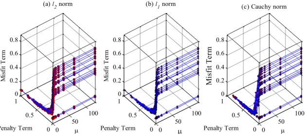
As shown in Fig. 5, for the narrowband case, the L-curves are computed with the slowness range of 0 <
22
𝑝 <2.56 𝜇s ∙ 𝑚𝑚−1 and frequency 0.1 < 𝑓 <0.7 MHz. A group of stable L-curves is obtained with values
23
of the hyperparameter 𝜇 = 0.001, 0.001 and 0.015 for 𝑙2-norm, 𝑙1-norm and Cauchy norm, respectively.
24
Thus, for Case I (see Fig. 1), both high resolution and noise filtering can be achieved using LRT methods
25
with a fixed μ value for all frequencies.
26
The L-curves obtained from the signals of a 2.5 mm-thick human bone ex vivo (case II) are depicted in
27
Fig. 6, with the slowness and frequency ranges of 0 < 𝑝 <2.56 𝜇s ∙ 𝑚𝑚−1 and 1.1 < 𝑓 <1.6 MHz.
28
According to the L-curves, small hyperparameter values of 𝜇 < 1 are still preferable for this case.
29
However, different from Fig. 5, even using such a small 𝜇 value, most of the penalty terms are still obtained
30
with the values below 0.01, which actually indicates the “all-zero” solutions. Such a result explains why in
31
Fig. 4, mode enhancement cannot be achieved by using the LRT methods in bandwidth of 1.1 < 𝑓 < 1.6
32
MHz.
33
(2) SNR threshold of the SVD-based method
34
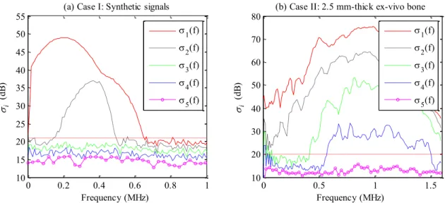
The performance of the SVD-based method mainly depends on the singular value selection, which can
35
be optimized by a SNR threshold. Fig. 7 presents the 5 singular values 𝜎𝑖 as functions of the frequency in
36
dB scale, where the signals are obtained in (a) case I: synthetic signals, narrow wavenumber-band Lamb
37
modes A0 and S0 on a 2 mm-thick Sawbones plate (see Fig. 1), and (b) case II: 2.5 mm-thick human bone
38
ex vivo (see Fig. 4). Our typical experimental signals are recorded with general SNR around 60 dB, but for
39
some low-amplitude modes, the SNR can be less than 10 dB, for example, the 𝜎4(𝑓) in dash line between
40
0.5 MHz and 1 MHz (Fig. 7b). It can be found that in both cases, SNR thresholds can be heuristically
41
determined from the 𝜎𝑖 functions.
42
B. Application Condition
43
For guided signals measured on a relatively large reception length (> 50 mm), the 2D-FT method is able
44
to characterize the dispersion curves of several fundamental Lamb modes, e.g., S0, A0 and S1 in the plate
model, or longitudinal guided modes, e.g., L(0,1), L(0,2), and L(0,3) in the cylindrical model 43,44. However,
1
the limited spatial sampling achievable with clinical probes (typically a few cm-long transducer arrays)
2
results in a poor wavenumber resolution with the consequence that only high-amplitude and
3
non-overlapped modes can be readily identified using the classical 2D-FT method. Such a limitation of the
4
2D-FT method can be improved by using the LRT methods and SVD-based method. However, different
5
application conditions of the two methods should be taken into account.
6
(1) LRT methods
7
The merits of the LRT methods originate from the theory of the Radon transform. The linear-path
8
functions, i.e., wave-packets in rays, can be projected to the Radon domain as different energy foci along
9
the linear slant-stack operator. Furthermore, the inversion based sparse technique, so-called high-resolution
10
LRT method, can be employed to sharpen the 𝜏﹣𝑝 and 𝑘﹣𝑓 resolution. As a result, only the less
11
dispersive modes with clear temporal rays can be concentrated as foci by using high-resolution LRT
12
methods with sparsity.
13
For case I (see Fig. 1), if the wave-packets actually propagate at significantly different velocities and if
14
the temporal overlapping is mainly caused by the short propagation distance instead of dispersion, then the
15
modes can be perfectly separated by the slowness range selection in the Radon domain. Furthermore,
16
considering the reversibility of the LRT method between (𝑘, 𝑓) and (𝑥, 𝑡) fields, the LRT method is
17
capable of providing another good solution to separate some narrowband modes, for example, to extract the
18
slowest fundamental A0 modes in long bone 29. The extraction of A0 mode in 𝜏﹣𝑝 field might be more
19
efficient than the temporal wave-packets extraction using the so-called group velocity mask filtering 45.
20
However, for case II (Figs. 2 and 4), i.e., wideband multimodal signals with high attenuation and
21
dispersion, it has been shown that the LRT methods can only enhance the resolution of some
22
high-amplitude modes close to the center frequency of the probe, which actually fails to achieve a
23
wideband dispersion curves extraction.
24
For case III (Fig. 3), the axial transmission signals, measured from the 25.5 mm-thick PMMA plate,
25
mainly consist of non-dispersive body waves, which are similar to the seismic signals measured from the
26
large-scale media with multiple ray-paths. The LRT methods are able to extract the individual temporal
27
wave-packets propagating along different paths, even for the reflected signals with low amplitudes. The
28
slowness of each wave-packet can be directly read from the τ-p domain. The results suggest that the LRT
29
methods are suitable for extracting FAS 6 and other multipath body waves 9 in the long bone.
30
A beamforming and angle steering strategy at the emission stage can be used to obtain the ultrasonic
31
guided modes with narrowband phase velocity spectrum leading to relatively clear ray contributions in the
32
distance-time diagram 46. For instance, the phase velocities of the multimode signals are approximately in a
33
range of 3 to 5 𝜇s ∙ 𝑚𝑚−128. In such case, although mode dispersion and temporal overlapping exist, 34
because of the presence of relatively clear rays for the different modes, the high-resolution LRT method
35
can still be used to improve the resolution of 𝑘﹣𝑓 dispersion curves imaging. However, without enough
36
enhancement of the low-amplitude modes, the LRT methods usually provide identical maxima loci in
37
comparison to 2D-FT. Regarding the identification of those modes with high dispersion and weak
38
amplitude in wide 𝑘﹣𝑓 ranges, e.g., S1 and S2 modes in Fig. 4, some improvements are still necessary.
39
We found that (1) the high-resolution LRT methods can enhance the 𝑘﹣𝑓 resolution of some modes
40
with narrow velocity range, e.g., two fundamental Lamb modes (S0 and A0) in Figs.1 e-f and S0, A0 and
41
A1 and S1 modes in Fig. 4e; (2) in contrast, for wideband highly-dispersive and low-amplitude modes, it is
42
still challenging to concentrate 𝑘﹣𝑓 trajectories using the LRT methods, e.g., for guided waves signals in
43
Figs. 2 and 4 corresponding to case II. The sparse assumption of the Radon projection of the linear events in
44
the (𝑥, 𝑡) field is well satisfied when different wave-packets propagate at constant velocities (Fig. 3 case
III). For the multimode signals with severe dispersion, the assumption is valid, when there are still clear
1
linear events in (𝑥, 𝑡) domain, for instance, signals with only S0 and A0 modes in Fig. 1 (case I) and some
2
seismic data presented in 34,47,48. However, for case II, both the dispersion and short propagation distances
3
of a few centimeters are responsible for modes overlapping for wavenumbers ranging from 0 to 5 𝑟𝑎𝑑 ∙
4
𝑚𝑚−110,28,29. As a consequence, there is no clear linear events observed in the wideband multimode 5
signals (see Figs. 2 and 4), so that the low-amplitude signals cannot be effectively enhanced by using the
6
slant-stack operator of the LRT methods. Such a challenge causes the inefficiency of the sparse penalty
7
term, i.e., norm of the 𝑊(𝑝, 𝑓), involved in the LRT methods (Fig. 6). It could explain the difficulties
8
during our application of the LRT methods for extracting the wideband dispersion curves, in particular for
9
the low-amplitude multimode signals under a poor SNR (case II Figs. 2 and 4).
10
(2) SVD-based method
11
For both narrowband (case I) and wideband (case II) guided signals, the multi-emitter and
12
multi-receiver configuration combined with the singular vectors selection strategy of the SVD allows
13
achieving a stable performance for noise filtering and extraction of the dispersion curves.
14
C. Other Potential Approaches and Improvements
15
Many classical spectra estimation methods 49, such as the Burg method or the multiple signal
16
classification method (MUSIC), can be used to achieve high-resolution wavenumber estimation. Recently,
17
sparse methods have been introduced for dispersion curves extraction. Harley et al. 26 have proposed a
18
compressed-sensing-based sparse wavenumber method for the recovery of the dispersion curves. These
19
authors showed that the sparse penalty regularization can be directly performed using the wavenumber
20
penalty. Such a sparse strategy in the (𝑘, 𝑓) field may be more efficient and convenient. Currently, the
21
sparse wavenumber extraction method proposed by Harley et al. has been verified on aluminum metal
22
plates 26. The practical challenge encountered with axial transmission in cortical bone is to efficiently
23
enhance the weak modes under the conditions of severe broadband overlapping (more than 5 modes in
24
some frequency band, see Fig. 4). The sparse singular value decomposition (S-SVD) technique, i.e., an
25
improved SVD-based method by using the sparse strategy in (𝑘, 𝑓) rather than the (𝜏, 𝑝) domain, may
26
significantly overcome the limitation of poor wavenumber resolution 37,50. Other improvements for 3D
27
multi-emitter and multi-receiver space-time signal processing, e.g., high-dimensional seismic data
28
processing 51, might be also helpful for guided waves dispersion analysis, but the application has not been
29
reported in community of ultrasonic bone evaluation to date. In addition, other guided modes excitation
30
technology, e.g., coded excitation52-54 and wideband dispersion reversal method55 etc., can also be helpful
31
to enhance the SNR of the ultrasonic axial transmission signals in the long cortical bone.
32
Generally speaking, in order to interpret the relatively complex guided signals, the signal processing
33
methods should be robust enough to allow the wideband dispersion curve extraction and the low-amplitude
34
mode detection. By retaining the singular values above noise level, the SVD-based method significantly
35
enhances the weak mode extraction when they are poorly detected by the 2D-FT method and LRT methods.
36
In this sense, the SVD-based method could be more suitable for signal processing of the ultrasonic guided
37
waves in the long bone, especially for highly dispersive wideband signals, in presence of severe attenuation
38
and low SNR.
39
VI. CONCLUSION 40
Different signal processing methods are necessary to cover the entire cortical bone thickness range of
41
the human long bone. The LRT methods have the advantage of the reversibility between (𝜏, 𝑝) and (𝑥, 𝑡)
42
fields showing a good ability to separate modes with large velocity difference, which is suitable for data
43
analysis of ultrasonic guided waves at low 𝑓 ∙ ℎ range (𝑓 ∙ ℎ < 1 MHz ∙ 𝑚𝑚), e.g., signals consisting of two
44
fundamental modes S0 and A0 with a large velocity difference presented in the study (Fig. 1). For the
45
highly dispersive multimode signals in a broadband 𝑓 ∙ ℎ range (0<𝑓 ∙ ℎ < 6 MHz ∙ 𝑚𝑚), which are quite
usual in the axial transmission measurement of the human long bone (Figs. 2 and 4), the SVD-based
1
method shows more robust performances for weak mode enhancement and noise filtering. Finally,
2
regarding computation time, the SVD-based method can be accomplished efficiently without any iterations,
3
but the 𝑙1-norm and Cauchy norm LRT methods are relatively time-consuming due to the reweighting
4
strategy at each frequency.
5
Future work will be to improve the resolution of the SVD method using the sparse strategy, i.e., recently
6
proposed S-SVD method 37,50, which may achieve a high-resolution extraction of the dispersion curves of 7
ultrasonic guided waves.
8
ACKNOWLEDGMENT 9
The authors also acknowledge Dr. Maryline Talmant for her constructive comments and excellent
10
advices to improve the paper. This work was supported by the National Natural Science Foundation of
11
China (11304043, 11327405, 11525416), the NSFC-CNRS-PICS (11511130133) and the CNRS PICS
12
programme n°07032.
13 14
1
References:
21 M. Talmant, J. Foiret and J. G. Minonzio, "Guided Waves in Cortical Bone," Bone Quantitative Ultrasound, 147-179 (2011).
3
2 P. Moilanen, "Ultrasonic guided waves in bone," IEEE Trans. Ultrason. Ferroelectr. Freq. Control 55, 1277-1286 (2008).
4
3 R. Barkmann, E. Kantorovich, C. Singal, D. Hans, H. K. Genant, M. Heller, and C. C. Gluer, "A new method for quantitative
5
ultrasound measurements at multiple skeletal sites - First Results of precision and fracture discrimination D-1837-2010 6
C-9752-2010," J. Clin. Densitom. 3, 1-7 (2000). 7
4 V. C. Protopappas, M. G. Vavva, D. I. Fotiadis, and K. N. Malizos, "Ultrasonic monitoring of bone fracture healing," IEEE
8
Trans. Ultrason. Ferroelectr. Freq. Control 55, 1243-1255 (2008). 9
5 K. Xu, D. Ta, R. He, Y. Qin, and W. Wang, "Axial transmission method for long bone fracture evaluation by ultrasonic
10
guided waves: Simulation, phantom and in vitro experiments," Ultrasound Med. Biol. 40, 817-827 (2014). 11
6 A. J. Foldes, A. Rimon, D. D. Keinan, and M. M. Popovtzer, "Quantitative ultrasound of the tibia: a novel approach for
12
assessment of bone status," Bone 17, 363-367 (1995). 13
7 P. H. F. Nicholson, P. Moilanen, T. Karkkainen, J. Timonen, and S. L. Cheng, "Guided ultrasonic waves in long bones:
14
Modelling, experiment and in vivo application," Physiol. Meas. 23, 755-768 (2002). 15
8 J. G. Minonzio, M. Talmant and P. Laugier, "Guided wave phase velocity measurement using multi-emitter and
16
multi-receiver arrays in the axial transmission configuration," J. Acoust. Soc. Am. 127, 2913-2919 (2010). 17
9 L. H. Le, Y. J. Gu, Y. P. Li, and C. Zhang, "Probing long bones with ultrasonic body waves," Appl. Phys. Lett. 96(11410211),
18
1-3 (2010). 19
10 Q. Vallet, N. Bochud, C. Chappard, P. Laugier, and J. Minonzio, "In vivo characterization of cortical bone using guided
20
waves measured by axial transmission," IEEE Trans. Ultrason. Ferroelectr. Freq. Control, DOI 10.1109/TUFFC.2016.2587079 21
(2016). 22
11 V. Kilappa, K. Xu, P. Moilanen, E. Heikkola, D. Ta, and J. Timonen, "Assessment of the fundamental flexural guided wave
23
in cortical bone by an ultrasonic axial-transmission array transducer," Ultrasound Med. Biol. 39, 1223-1232 (2013). 24
12 A. Tatarinov, V. Egorov, N. Sarvazyan, and A. Sarvazyan, "Multi-frequency axial transmission bone ultrasonometer,"
25
Ultrasonics 54, 1162-1169 (2014). 26
13 X. Song, D. Ta and W. Wang, "Analysis of superimposed ultrasonic guided waves in long bones by the joint approximate
27
diagonalization of eigen-matrices algorithm," Ultrasound Med. Biol. 37, 1704-1713 (2011). 28
14 J. Foiret, J. G. Minonzio, C. Chappard, M. Talmant, and P. Laugier, "Combined estimation of thickness and velocities using
29
ultrasound guided waves: a pioneering study on in vitro cortical bone samples," IEEE Trans. Ultrason. Ferroelectr. Freq. 30
Control 61, 1478-1488 (2014). 31
15 C. H. Chapman, "A new method for computing synthetic seismograms," Geophys. J. Int. 54, 481-518 (1978).
32
16 J. Hong, K. H. Sun and Y. Y. Kim, "Dispersion-based short-time Fourier transform applied to dispersive wave analysis," J.
33
Acoust. Soc. Am. 117, 2949-2960 (2005). 34
17 P. Moilanen, P. Nicholson, V. Kilappa, S. L. Cheng, and J. Timonen, "Assessment of the cortical bone thickness using
35
ultrasonic guided waves: Modelling and in vitro study," Ultrasound Med. Biol. 33, 254-262 (2007). 36
18 V. C. Protopappas, I. C. Kourtis, L. C. Kourtis, K. N. Malizos, C. V. Massalas, and D. I. Fotiadis, "Three-dimensional finite
37
element modeling of guided ultrasound wave propagation in intact and healing long bones," J. Acoust. Soc. Am. 121, 38
3907-3921 (2007). 39
19 L. De Marchi, A. Marzani, S. Caporale, and N. Speciale, "Ultrasonic guided-waves characterization with warped frequency
40
transforms," IEEE Trans. Ultrason. Ferroelectr. Freq. Control 56, 2232-2240 (2009). 41
20 K. Xu, D. Ta and W. Wang, "Multiridge-based analysis for separating individual modes from multimodal guided wave
42
signals in long bones," IEEE Trans. Ultrason. Ferroelectr. Freq. Control 57, 2480-2490 (2010). 43
21 Z. Zhang, K. Xu, D. Ta, and W. Wang, "Joint spectrogram segmentation and ridge-extraction method for separating
44
multimodal guided waves in long bones," Science China Physics, Mechanics and Astronomy 56(7), 1317-1323 (2013). 45
22 K. Xu, D. Ta, P. Moilanen, and W. Wang, "Mode separation of Lamb waves based on dispersion compensation method," J.
46
Acoust. Soc. Am. 131, 2714-2722 (2012). 47
23 Y. Yang, Z. K. Peng, W. M. Zhang, G. Meng, and Z. Q. Lang, "Dispersion analysis for broadband guided wave using
48
generalized warblet transform," J. Sound Vib. 367, 22-36 (2016). 49
24 L. Zeng, M. Zhao, J. Lin, and W. Wu, "Waveform separation and image fusion for Lamb waves inspection resolution
50
improvement," NDT&E Int. 79, 17-29 (2016). 51
25 M. Ratassepp, A. Klauson, F. Chati, F. Léon, D. Décultot, G. Maze, and M. Fritzsche, "Application of orthogonality-relation
52
for the separation of Lamb modes at a plate edge: Numerical and experimental predictions," Ultrasonics 57, 90-95 (2015). 53
26 J. B. Harley and J. M. F. Moura, "Sparse recovery of the multimodal and dispersive characteristics of Lamb waves," J.
54
Acoust. Soc. Am. 133, 2732 (2013). 55
27 J. G. Minonzio, J. Foiret, M. Talmant, and P. Laugier, "Impact of attenuation on guided mode wavenumber measurement in
56
axial transmission on bone mimicking plates," J. Acoust. Soc. Am. 130, 3574-3582 (2011). 57
28 T. N. Tran, K. T. Nguyen, M. D. Sacchi, and L. H. Le, "Imaging ultrasonic dispersive guided wave energy in long bones
using linear Radon transform," Ultrasound Med. Biol. 40, 2715-2727 (2014). 1
29 T. N. Tran, L. H. Le, M. D. Sacchi, V. Nguyen, and E. H. Lou, "Multichannel filtering and reconstruction of ultrasonic
2
guided wave fields using time intercept-slowness transform," J. Acoust. Soc. Am. 136, 248-259 (2014). 3
30 C. H. Chapman, "Generalized Radon transforms and slant stacks," Geophys. J. Int. 66, 445-453 (1981).
4
31 M. D. Sacchi, "Statistical and transform methods in geophysical signal processing,"
5
https://www.ualberta.ca/~msacchi/Notes.pdf, 209-253 (2002). 6
32 J. R. Thorson and J. F. Claerbout, "Velocity-stack and slant-stack stochastic inversion," Geophysics 50, 2727-2741 (1985).
7
33 M. D. Sacchi and T. J. Ulrych, "High-resolution velocity gathers and offset space reconstruction," Geophysics 60, 1169
8
(1995). 9
34 Y. Luo, J. Xia, R. D. Miller, Y. Xu, J. Liu, and Q. Liu, "Rayleigh-wave dispersive energy imaging using a high-resolution
10
linear Radon transform," Pure Appl. Geophys. 165, 903-922 (2008). 11
35 I. A. Viktorov, Rayleigh and Lamb waves: physical theory and applications, 67-75 (Plenum press New York, 1967).
12
36 Z. Su, L. Ye and Y. Lu, "Guided Lamb waves for identification of damage in composite structures: a review," J. Sound Vib.
13
295, 753-780 (2006). 14
37 K. Xu, J. Minonzio, D. Ta, B. Hu, W. Wang, and P. Laugier, "Sparse SVD Method for High Resolution Extraction of the
15
Dispersion Curves of Ultrasonic Guided Waves," IEEE Trans. Ultrason. Ferroelectr. Freq. Control, DOI: 16
10.1109/TUFFC.2016.2592688 (2016). 17
38 L. Moreau, J. G. Minonzio, M. Talmant, and P. Laugier, "Measuring the wavenumber of guided modes in waveguides with
18
linearly varying thickness," J. Acoust. Soc. Am. 135, 2614-2624 (2014). 19
39 R. Schultz and Y. Jeffrey Gu, "Flexible, inversion-based Matlab implementation of the Radon transform," Comput.
20
Geosci.-UK 52, 437-442 (2013). 21
40 M. D. Sacchi, "Reweighting strategies in seismic deconvolution," Geophys. J. Int. 129, 651-656 (1997).
22
41 W. H. Press, S. A. Teukolsky, W. T. Vetterling, and B. P. Flannery, Numerical recipes 2nd edition: The art of scientific
23
computing, 402-405 (Cambridge university press, 1992).
24
42 H. W. Engl and W. Grever, "Using the L-curve for determining optimal regularization parameters," Numer. Math. 69, 25-31
25
(1994). 26
43 F. Lefebvre, Y. Deblock, P. Campistron, D. Ahite, and J. J. Fabre, "Development of a new ultrasonic technique for bone and
27
biomaterials in vitro characterization," J. Biomed. Mater. Res. 63, 441-446 (2002). 28
44 D. Ta, K. Huang, W. Wang, Y. Wang, and L. H. Le, "Identification and analysis of multimode guided waves in tibia cortical
29
bone," Ultrasonics 44, e279-e284 (2006). 30
45 P. Moilanen, P. Nicholson, V. Kilappa, S. Cheng, and J. Timonen, "Measuring guided waves in long bones: Modeling and
31
experiments in free and immersed plates," Ultrasound Med. Biol. 32, 709-719 (2006). 32
46 J. J. Ditri and J. L. Rose, "Excitation of guided waves in generally anisotropic layers using finite sources," Journal of applied
33
mechanics 61, 330-338 (1994). 34
47 L. Wang, Y. Xu, J. Xia, and Y. Luo, "Effect of near-surface topography on high-frequency Rayleigh-wave propagation," J.
35
Appl. Geophys. 116, 93-103 (2015). 36
48 J. Xia, Y. Xu and R. D. Miller, "Generating an image of dispersive energy by frequency decomposition and slant stacking,"
37
Pure Appl. Geophys. 164, 941-956 (2007). 38
49 F. Castanié, Spectral Analysis: parametric and non-parametric digital methods, 151-257 (John Wiley & Sons, 2010).
39
50 K. Xu, J. G. Minonzio, D. Ta, B. Hu, W. Wang, and P. Laugier, Sparse inversion SVD method for dispersion extraction of
40
ultrasonic guided waves in cortical bone, in Corfu, 2015, p. 1-3.
41
51 S. Yu, J. Ma, X. Zhang, and M. D. Sacchi, "Interpolation and denoising of high-dimensional seismic data by learning a tight
42
frame," Geophysics 80, V119-V132 (2015). 43
52 X. Song, D. Ta and W. Wang, "A base-sequence-modulated Golay code improves the excitation and measurement of
44
ultrasonic guided waves in long bones," IEEE Trans. Ultrason. Ferroelectr. Freq. Control 59, 2580-2583 (2012). 45
53 J. Lin, J. Hua, L. Zeng, and Z. Luo, "Excitation Waveform Design for Lamb Wave Pulse Compression," IEEE Trans.
46
Ultrason. Ferroelectr. Freq. Control 63, 165 - 177 (2015). 47
54 M. Yucel, S. Fateri, M. Legg, A. Wilkinson, V. Kappatos, C. Selcuk, and T. Gan, "Coded waveform excitation for high
48
resolution ultrasonic guided wave response," IEEE T. Ind. Inform., 1-1 (2016). 49
55 K. Xu, D. Ta, B. Hu, P. Laugier, and W. Wang, "Wideband dispersion reversal of Lamb waves," IEEE Trans. Ultrason.
50
Ferroelectr. Freq. Control 61, 997-1005 (2014). 51
56 P. Moilanen, M. Talmant, V. Bousson, P. Nicholson, S. Cheng, J. Timonen, and P. Laugier, "Ultrasonically determined
52
thickness of long cortical bones: Two-dimensional simulations of in vitro experiments," J. Acoust. Soc. Am. 122, 1818-1826 53
(2007). 54
57 K. T. Nguyen, L. H. Le, T. N. Tran, M. D. Sacchi, and E. H. Lou, "Excitation of ultrasonic Lamb waves using a phased array
55
system with two array probes: Phantom and in vitro bone studies," Ultrasonics 54, 1178-1185 (2014). 56
58 E. Bossy, M. Talmant and P. Laugier, "Three-dimensional simulations of ultrasonic axial transmission velocity measurement
57
on cortical bone models," J. Acoust. Soc. Am. 115, 2314-2324 (2004). 58
59 J. Chen, J. Foiret, J. G. Minonzio, M. Talmant, Z. Su, L. Cheng, and P. Laugier, "Measurement of guided mode
wavenumbers in soft tissue-bone mimicking phantoms using ultrasonic axial transmission," Phys. Med. Biol. 57, 3025-3037 1
(2012). 2
60 J. G. Minonzio, J. Foiret, P. Moilanen, J. Pirhonen, Z. Zhao, M. Talmant, J. Timonen, and P. Laugier, "A free plate model can
3
predict guided modes propagating in tubular bone-mimicking phantoms," J. Acoust. Soc. Am. 137, EL98-EL104 (2015). 4
61 P. Moilanen, M. Talmant, V. Kilappa, P. Nicholson, S. L. Cheng, J. Timonen, and P. Laugier, "Modeling the impact of soft
5
tissue on axial transmission measurements of ultrasonic guided waves in human radius," J. Acoust. Soc. Am. 124, 2364-2373 6
(2008). 7
62 L. Cohen, "Time-frequency distributions-a review," P. IEEE 77, 941-981 (1989).
8
63 J. Cardoso and A. Souloumiac, Blind beamforming for non-Gaussian signals, 1993 (IET), p. 362-370.
9 10 11
List of tables: 1
Table I. Characteristics of ultrasonic signals in the long cortical bone at different 𝒇 ∙ 𝒉 ranges 2
frequency-thickness product (𝑓 ∙ ℎ) (MHz ∙
𝑚𝑚)
Case I Case II Case III
𝑓 ∙ ℎ < 1 1 < 𝑓 ∙ ℎ < 6 6 < 𝑓 ∙ ℎ
Signal characteristics 1. Two fundamental guided modes are measured, i.e., a small amplitude and fast wave-packet
(symmetric S0) and a high amplitude and slow wave-packet (asymmetric A0); 2. Speed values are
different enough so that the two wave-packets do not overlap in time even for relatively short propagation distances (a few cm).
3. The dispersion
information of the lateral arrival A0 mode can be used to estimate cortical thickness 11,56.
1. Under the wideband excitation, more than 5 guided modes with overlapping velocity ranges;
2. For the relatively short propagation distances (a few cm) 8,12,18,44,57, a complete dispersion extraction of the overlapping multimode is still challenging. 1. Similar to many geophysical applications, mainly body waves with linear ray paths 9; 2. FAS is the lateral
wave propagating at the bulk compression velocity 7,58;
3. Velocities of S0 and A0 modes converge to the Rayleigh velocity. Velocities of other guided modes converge to the shear velocity 35.
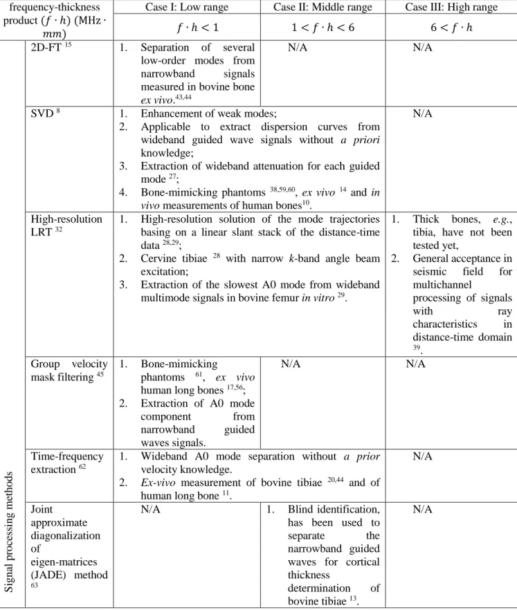
Table II. Signal processing methods for assessment of the long cortical bone using axial transmission 1
frequency-thickness product (𝑓 ∙ ℎ) (MHz ∙
𝑚𝑚)
Case I: Low range Case II: Middle range Case III: High range 𝑓 ∙ ℎ < 1 1 < 𝑓 ∙ ℎ < 6 6 < 𝑓 ∙ ℎ Si g na l p roc es si n g m et ho d s 2D-FT 15 1. Separation of several low-order modes from narrowband signals measured in bovine bone ex vivo.43,44
N/A N/A
SVD 8 1. Enhancement of weak modes;
2. Applicable to extract dispersion curves from wideband guided wave signals without a priori knowledge;
3. Extraction of wideband attenuation for each guided mode 27;
4. Bone-mimicking phantoms 38,59,60, ex vivo 14 and in vivo measurements of human bones10.
N/A
High-resolution LRT 32
1. High-resolution solution of the mode trajectories basing on a linear slant stack of the distance-time data 28,29;
2. Cervine tibiae 28 with narrow k-band angle beam excitation;
3. Extraction of the slowest A0 mode from wideband multimode signals in bovine femur in vitro 29.
1. Thick bones, e.g., tibia, have not been tested yet,
2. General acceptance in seismic field for multichannel processing of signals with ray characteristics in distance-time domain 39. Group velocity mask filtering 45 1. Bone-mimicking phantoms 61, ex vivo human long bones 17,56; 2. Extraction of A0 mode component from narrowband guided waves signals. N/A N/A Time-frequency extraction 62
1. Wideband A0 mode separation without a prior velocity knowledge.
2. Ex-vivo measurement of bovine tibiae 20,44 and of human long bone 11.
N/A Joint approximate diagonalization of eigen-matrices (JADE) method 63
N/A 1. Blind identification,
has been used to
separate the
narrowband guided waves for cortical thickness
determination of bovine tibiae 13.
N/A
N/A: to the best knowledge of the authors, it has not been reported in the literatures of cortical bone guided waves 2
processing.
3 4 5
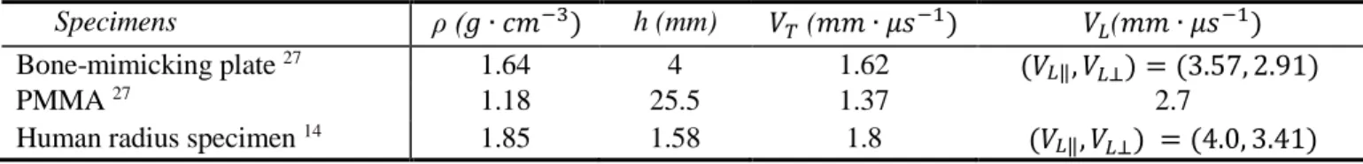
Table III. Shear and longitudinal velocities, density and thickness of the specimens used in experiments 1 Specimens ρ (𝑔 ∙ 𝑐𝑚−3) h (mm) 𝑉𝑇 (𝑚𝑚 ∙ 𝜇𝑠−1) 𝑉𝐿(𝑚𝑚 ∙ 𝜇𝑠−1) Bone-mimicking plate 27 1.64 4 1.62 (𝑉 𝐿‖, 𝑉𝐿⊥) = (3.57, 2.91) PMMA 27 1.18 25.5 1.37 2.7
Human radius specimen 14 1.85 1.58 1.8 (𝑉
𝐿‖, 𝑉𝐿⊥) = (4.0, 3.41)
2 3
List of figure captions: 1
2
Fig. 1. (color online) Synthetic signals, narrow wavenumber-band Lamb modes A0 and S0 on a 2
3
mm-thick Sawbone plate with peak-to-peak amplitudes of 1 and 0.3, and SNR of 30dB, (a)
4
distance-time diagram of the array-signals, (b) 2D-FT 𝑘﹣𝑓 result, (c) SVD 𝑘﹣𝑓 result, (d) the 𝜏﹣𝑝
5
energy distributions obtained by LRT with 𝑙2-norm, and 𝑘﹣𝑓 results obtained by LRT with
6
high-resolution regularization strategies, i.e., (e) 𝑙1-norm, (f) Cauchy norm, respectively.
7 8
1
2
Fig. 2. (color online) Experimental signals measured in a 4 mm-thick bone-mimicking plate, (a)
3
distance-time diagram of the array-signals, (b) 2D-FT 𝑘﹣𝑓 result, (c) SVD 𝑘﹣𝑓 result, (d) the 𝜏﹣𝑝
4
energy distributions obtained by LRT with 𝑙2-norm, and 𝑘﹣𝑓 results obtained by LRT with high
5
resolution regularization strategies, i.e., (e) 𝑙1-norm, (f) Cauchy norm, respectively.
6 7
1
2
Fig. 3. (color online) Experimental signals measured in the 25.5 mm-thick PMMA plate, (a)
3
distance-time diagram of the synthetic array-signals, (b) 2D-FT 𝑘﹣𝑓 mode energy distribution, (c)
4
SVD k-f mode energy distribution, (d) the 𝜏﹣𝑝 energy distributions obtained by LRT with 𝑙2-norm,
5
and 𝑘﹣𝑓 energy distributions obtained by LRT with high resolution regularization strategies, i.e., (e)
6
𝑙1-norm, (f) Cauchy norm, respectively.
7 8
1
2
Fig. 4. (color online) Experimental guided signals measured in the 2.5 mm-thick ex-vivo human radius,
3
(a) distance-time diagram of the synthetic array-signals, (b) 2D-FT 𝑘﹣𝑓 mode energy distribution, (c)
4
SVD 𝑘﹣𝑓 mode energy distribution, (d) the 𝜏﹣𝑝 energy distributions obtained by LRT with
5
𝑙2-norm, and 𝑘﹣𝑓 energy distributions obtained by LRT with high resolution regularization
6
strategies, i.e., (e) 𝑙1-norm, (f) Cauchy norm, respectively.
7 8
1
2
Fig. 5. (color online) L-curves of the synthetic signals (case I shown in Fig. 1), i.e., narrow
3
wavenumber-band Lamb modes A0 and S0 on a 2-mm-thick Sawbones plate, (a) 𝑙2-norm, (b) 𝑙1-norm,
4
(c) Cauchy norm. The slowness 𝑝 and frequency f range from 0 to 2.56 𝜇s ∙ 𝑚𝑚−1 and 0.1 to 0.7 MHz,
5 respectively. 6 7 0 50 100 0 0.5 10 0.2 0.4 0.6 0.8 (a) l2 norm Penalty Term M is fi t T er m 0 50 100 0 0.5 10 0.2 0.4 0.6 0.8 (b) l1 norm Penalty Term M is fi t T er m 0 50 100 0 0.5 10 0.2 0.4 0.6 0.8 (c) Cauchy norm Penalty Term M is fi t T er m