Seasonal evolution of C2N2, C3H4, and C4H2 abundances in Titan’s lower stratosphere

HAL Id: hal-01923403

https://hal.archives-ouvertes.fr/hal-01923403

Submitted on 16 Jan 2021

HAL is a multi-disciplinary open access

archive for the deposit and dissemination of

sci-entific research documents, whether they are

pub-lished or not. The documents may come from

teaching and research institutions in France or

abroad, or from public or private research centers.

L’archive ouverte pluridisciplinaire HAL, est

destinée au dépôt et à la diffusion de documents

scientifiques de niveau recherche, publiés ou non,

émanant des établissements d’enseignement et de

recherche français ou étrangers, des laboratoires

publics ou privés.

Seasonal evolution of C2N2, C3H4, and C4H2

abundances in Titan’s lower stratosphere

M. Sylvestre, N. Teanby, S. Vinatier, Sébastien Lebonnois, P. Irwin

To cite this version:

M. Sylvestre, N. Teanby, S. Vinatier, Sébastien Lebonnois, P. Irwin. Seasonal evolution of C2N2,

C3H4, and C4H2 abundances in Titan’s lower stratosphere. Astronomy and Astrophysics - A&A,

EDP Sciences, 2018, 609, pp.A64. �10.1051/0004-6361/201630255�. �hal-01923403�

A&A 609, A64 (2018) DOI:10.1051/0004-6361/201630255 c ESO 2018

Astronomy

&

Astrophysics

Seasonal evolution of C

2

N

2

, C

3

H

4

, and C

4

H

2

abundances in Titan’s

lower stratosphere

M. Sylvestre

, N. A. Teanby

, S. Vinatier

, S. Lebonnois

, and P. G. J. Irwin

1 _{School of Earth Sciences, University of Bristol, Wills Memorial Building, Queen’s Road, Bristol BS8 1 RJ, UK} e-mail: melody.sylvestre@bristol.ac.uk

2 _{LESIA, Observatoire de Paris, PSL Research University, CNRS, Sorbonne Universités, UPMC Univ. Paris 06, Univ. Paris Diderot,} Sorbonne Paris Cité, 5 Place Jules Janssen, 92190 Meudon, France

3 _{LMD, CNRS, IPSL, UMR 8539, 4 Place Jussieu, 750005 Paris, France}

4 _{Atmospheric, Oceanic, & Planetary Physics, Department of Physics, University of Oxford, Clarendon Laboratory, Parks Road,} Oxford OX1 3PU, UK

Received 14 December 2016/ Accepted 29 August 2017

ABSTRACT

Aims.We study the seasonal evolution of Titan’s lower stratosphere (around 15 mbar) in order to better understand the atmospheric dynamics and chemistry in this part of the atmosphere.

Methods. We analysed Cassini/CIRS far-IR observations from 2006 to 2016 in order to measure the seasonal variations of three

photochemical by-products: C4H2, C3H4, and C2N2.

Results.We show that the abundances of these three gases have evolved significantly at northern and southern high latitudes since 2006. We measure a sudden and steep increase of the volume mixing ratios of C4H2, C3H4, and C2N2 at the south pole from 2012 to 2013, whereas the abundances of these gases remained approximately constant at the north pole over the same period. At northern mid-latitudes, C2N2and C4H2abundances decrease after 2012 while C3H4abundances stay constant. The comparison of these volume mixing ratio variations with the predictions of photochemical and dynamical models provides constraints on the seasonal evolution of atmospheric circulation and chemical processes at play.

Key words. planets and satellites: atmospheres – methods: data analysis

1. Introduction

Titan’s atmosphere undergoes a rich photochemistry, initiated by the dissociation of its most abundant constituents, N2 and

CH4. In the thermosphere and the ionosphere (at altitudes above

600 km or the 0.0001 mbar pressure level), these molecules are dissociated by solar UV and EUV photons, energetic pho-toelectrons, and high energy electrons from Saturn’s magne-tosphere (Wilson & Atreya 2004;Vuitton et al. 2012). Radicals and ions produced by these photodissociations react together and form hydrocarbons, nitriles, and eventually organic hazes. These species are then destroyed by photolysis or further chemical re-actions in the upper and middle atmosphere, or they condense in the lower part of the stratosphere (at altitudes inferior to 100 km or at pressures superior to 10 mbar). As Titan’s obliquity is 26.7◦, its atmosphere undergoes significant seasonal variations of insolation which are expected to affect the abundances of the photochemical by-products. In addition, this seasonal forc-ing affects atmospheric dynamics, which transports minor atmo-spheric constituents (Teanby et al. 2008a, 2012; Vinatier et al. 2015). Hence, measuring the meridional and vertical distribu-tions of the various photochemical species is a way to better un-derstand the photochemical and dynamical processes in Titan’s atmosphere.

Abundances of hydrocarbons and nitriles and their tem-poral evolution have been measured in various studies, es-pecially since the beginning of the Cassini mission in 2004. This spacecraft has provided thirteen years of observations of Titan at different wavelength ranges, enabling us to monitor

the seasonal evolution of its atmosphere throughout its north-ern winter and spring. During Titan’s northnorth-ern winter, limb and nadir observations performed with the infrared spectrom-eters Voyager 1/IRIS in November 1980 (Infrared Instru-ment,Hanel et al. 1981) and Cassini/Composite InfraRed Spec-trometer (CIRS; Flasar et al. 2004) between 2004 and 2008 showed that many species such as acetylene (C2H2),

diacety-lene (C4H2), or cyanoacetylene (HC3N) exhibited an enrichment

at high northern latitudes (Kunde et al. 1981; Coustenis et al. 1991, 2007, 2010; Teanby et al. 2008b; Vinatier et al. 2010; Bampasidis et al. 2012). This was attributed to the atmo-spheric circulation which took the form of a single pole-to-pole Hadley cell, and more specifically to the subsiding branch of this cell, located above the winter pole and bring-ing photochemical species from their production level to the stratosphere (Teanby et al. 2009b; Vinatier et al. 2010). Af-ter the equinox (August 2009), CIRS measurements analysed by Teanby et al. (2012), Coustenis et al. (2013), Vinatier et al. (2015), Coustenis et al. (2016) revealed that the vertical and meridional distributions of these gases have changed signifi-cantly, especially above the south pole where the abundances of photochemical by-products strongly increased after 2011. This was interpreted as a subsidence above high southern latitudes, due to the reversal of the pole-to-pole Hadley cell. At northern latitudes, Coustenis et al.(2013) found a decrease in trace gas abundances between 2010 and 2012.

While mid-infrared CIRS observations provide information between 10 mbar and 0.001 mbar for limb observations, and from 10 mbar to 0.5 mbar for nadir observations, far-infrared

CIRS spectra mainly probe the lower part of the stratosphere, at pressure levels between 10 mbar and 20 mbar. For instance, this type of observation allowedTeanby et al.(2009a) to measure the meridional distribution of diacetylene (C4H2) and

methylacety-lene (C3H4) in the lower stratosphere during winter.

Further-more, unlike the CIRS mid-infrared observations, far-infrared spectra can be used to measure the distribution of cyanogen (C2N2), thus providing additional information about the

chem-istry of Titan’s stratosphere. For instance,Teanby et al.(2009a) compared the enrichment in C2N2 and other nitriles and

hydro-carbons at the north pole during winter, and suggested that ni-triles undergo an additional loss process compared to the hydro-carbons with similar lifetimes, as proposed byYung(1987).

In this paper, we use nadir far-infrared spectra from Cassini/CIRS to measure the meridional distributions of diacety-lene (C4H2), methylacetylene (C3H4), and cyanogen (C2N2)

from 2006 to 2015. The data we present cover the whole lati-tude range and were acquired throughout the Cassini mission. It allows us to monitor precisely the seasonal evolution of the dis-tributions of C2N2, C3H4, and C4H2 in the lower stratosphere,

and thus to complete the previous studies by giving insights on the atmospheric dynamics and photochemistry of Titan’s lower stratosphere.

2. Observations

Cassini/CIRS (Flasar et al. 2004) is a Fourier transform spectrometer composed of three focal planes which operate in different wavenumber ranges. The focal plane FP1 probes the spectral range 10−600 cm−1 _{(17−1000 µm) and is made of a}

single circular detector with an angular resolution of 3.9 mrad. The focal planes FP3 and FP4 respectively measure spectra in

600−1100 cm−1 _{(9−17 µm) and 1100−1400 cm}−1 _{(7−9 µm).}

Both are composed of a linear array of ten detectors with an angular resolution of 0.273 mrad per detector.

In this study, we analyse nadir spectra acquired from FP1, with an apodised spectral resolution of 0.5 cm−1_{, in order to}

re-solve the spectral signatures of C2N2, C3H4, and C4H2. We also

exploit FP4 spectra acquired at the same resolution in order to measure temperature with the ν4CH4band (1304 cm−1). These

observations were made in “sit-and-stare” geometry, where each detector of FP1 and FP4 probes the same latitude and longitude throughout the acquisition, with a total integration time com-prised between 1h30 and 4h30. During these observations, the average spatial field of view is 20◦of latitude for the single de-tector of FP1, 2◦_{for each FP4 detector, and 15−20}◦_{for the whole}

FP4 array, depending on its orientation.

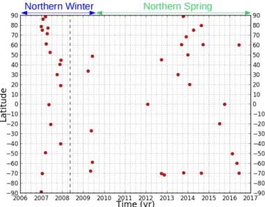
The datasets used in this study are summarised in TableA.1. We selected data covering the whole latitude range, acquired from 2006 to 2016 (see Fig.1), in order to get an overview of the seasonal evolution from northern winter to mid-spring. For each dataset, 100 to 330 spectra were acquired with FP1, and 500 to 1650 with FP4. We use the photometric calibration pro-vided by the CIRS team (version DS4000) which corrects the ef-fects of sky background and thermal noise of the detectors more effectively than the standard calibration. Some of the datasets acquired during northern winter (before 2008, see Table A.1) have already been presented inTeanby et al.(2009a), but as we use a different calibration version, we reanalyse them, to ensure a consistent comparison between these data and the other data presented in this study.

For each FP1 and FP4 dataset, all the spectra acquired are averaged together in order to improve the signal-to-noise ratio by √N (with N the number of averaged spectra). The average

Fig. 1.Spatial and temporal distribution of the FP1 data analysed in this paper. They cover all the latitudes, with a spatial field of view of 20◦_{. Observations are available for different times throughout northern} winter and spring. Their temporal distribution is controlled by the orbits of the Cassini spacecraft.

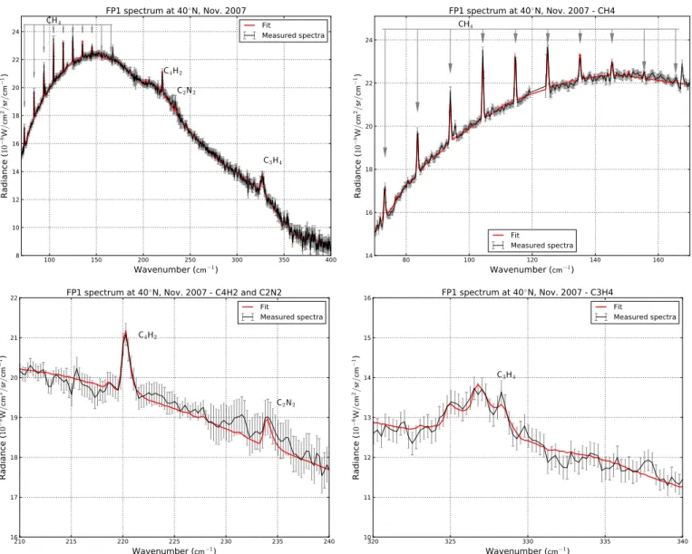
signal-to-noise ratio reaches 115 at 220 cm−1(spectra acquired with FP1) and 160 at 1300 cm−1_{(FP4 spectra). Figure2shows}

an example of spectrum obtained after averaging 271 FP1 spec-tra measured at 40◦_{N in November 2007.}

3. Analysis

In order to retrieve the abundances of C4H2, C2N2, and C3H4,

we use the constrained non-linear inversion code NEMESIS (Irwin et al. 2008). Retrievals are performed following an iter-ative process based on the generation of synthetic spectra from a reference atmosphere, and the minimisation of a cost function in order to find the value of the retrieved parameter which provides the best fit of the measured spectrum.

3.1. Reference atmosphere

Our reference atmosphere extends from 0 km (∼1438 mbar) to 780 km (∼1 × 10−5_{mbar). The gases included in this study, their}

abundances, and the studies in which they were measured are detailed in Table1. These measurements were performed using data from Cassini/CIRS (Nixon et al. 2012;Cottini et al. 2012; Teanby et al. 2009a; Coustenis et al. 2016), Huygens/GCMS (Niemann et al. 2010), Cassini/VIMS (Maltagliati et al. 2015), and ALMA (Molter et al. 2016). We set constant vertical pro-files for the constituents of our reference atmosphere above their respective condensation pressure level. In our model, the abun-dances of Titan’s atmospheric constituents do not depend on the considered latitude. However,Lellouch et al.(2014) showed that in the lower stratosphere (around 15 mbar) the CH4 mole

frac-tion varies significantly (from 1.0 to 1.5%), which can affect the temperatures and gas abundances retrieved in this study. We ad-dress this problem in Sect.3.6.

Spectroscopic data for the constituents of the refer-ence atmosphere come from the GEISA 2015 database (Jacquinet-Husson et al. 2016). The spectral contributions due to collisions induced absorption (CIA) between the main con-stituents of Titan’s atmosphere (N2, CH4, and H2) are calculated

M. Sylvestre et al.: Seasonal evolution of C2N2, C3H4, and C4H2 100 150 200 250 300 350 400 Wavenumber (cm−1) 8 10 12 14 16 18 20 22 24 Ra dia nc e ( 10 − 8W / cm 2/sr / cm − 1) C4H2 C2N2 C3H4 CH4 FP1 spectrum at 40◦N, Nov. 2007 Fit Measured spectra 80 100 120 140 160 Wavenumber (cm−1) 14 16 18 20 22 24 Ra dia nc e ( 10 − 8W / cm 2/sr / cm − 1) C4H2 C2N2 C3H4 CH4 FP1 spectrum at 40◦N, Nov. 2007 - CH4 Fit Measured spectra 210 215 220 225 230 235 240 Wavenumber (cm−1) 16 17 18 19 20 21 22 Ra dia nc e ( 10 − 8W / cm 2/sr / cm − 1) C4H2 C2N2

FP1 spectrum at 40◦N, Nov. 2007 - C4H2 and C2N2

Fit Measured spectra 320 325 330 335 340 Wavenumber (cm−1) 10 11 12 13 14 15 16 Ra dia nc e ( 10 − 8W / cm 2/sr / cm − 1) C3H4 CH4 FP1 spectrum at 40◦N, Nov. 2007 - C3H4 Fit Measured spectra

Fig. 2.Example of FP1 spectrum (after average). The top left panel shows the whole spectrum while the three other panels are a close-up around the relevant spectral bands. Measured spectra are in black. Red solid lines show the synthetic spectra calculated during the retrieval process. Data were acquired at a spectral resolution of 0.5 cm−1_{. Error bars of the FP1 spectrum have been corrected because the initial error bars were too small} with respect to the radiance variations caused by noise (see Sects.2and3.3). C4H2, C2N2, and C3H4bands are visible, and allow us to retrieve the volume mixing ratios of these species. The CH4bands in FP1 are used to retrieve the temperature profile between 20 mbar and 10 mbar.

Borysow & Tang (1993), and Borysow (1991). Following the studies ofTomasko et al.(2008a),de Kok et al.(2010), we mul-tiply the absorption coefficients of the CIA by 1.5.

Our reference atmosphere takes into account the broad spec-tral contributions of Titan’s stratospheric hazes. For the FP1 spectra (70−400 cm−1), we consider four types of hazes, follow-ing de Kok et al. (2007). The main feature (haze 0) covers all wavenumbers from 70 cm−1 to 550 cm−1. Its extinction profile has a scale height of 65 km from 80 km to 250 km and is constant below 80 km, following de Kok et al. (2010), Tomasko et al. (2008b). Three other localised features are also included: hazes A (centred at 140 cm−1_{), B (centred at 220 cm}−1_{), C (centred at}

190 cm−1) as described inde Kok et al.(2007). For the FP4 spec-tra (1200−1360 cm−1_{), we use the aerosols properties measured}

byVinatier et al.(2012).

3.2. Retrieval method

The retrievals are performed in several iterations. To retrieve a given variable (e.g. temperature profile, scale factor toward a given a priori vertical profile of a gas) at each iteration,

a synthetic spectrum is calculated by NEMESIS using the correlated-k method. Then, the difference between the synthetic and the measured spectra is used to compute an increment to add to the retrieved variable. At the next step, the new value or profile of this variable is then used to compute a new synthetic spectrum. This method is detailed inIrwin et al.(2008).

We retrieve simultaneously a continuous temperature profile, and best-fitting scales factors for the a priori vertical profiles of C2N2, C3H4, C4H2, hazes 0, A, B, and C from the FP1 spectra.

Hazes fit the continuum component of the spectra. Temperature is measured using the radiance in the ten CH4 rotational bands

between 70 cm−1_{and 170 cm}−1_{, and the continuum. Abundances}

of C4H2, C2N2, and C3H4 are obtained by fitting the radiance

in their respective spectral bands at 220 cm−1_{, 234 cm}−1_{, and}

327 cm−1.

For each retrieved physical quantity, we can assess the sen-sitivity of our measurements as a function of the pressure using the inversion kernels defined as

Ki j =

∂Ii

∂xj

Table 1. Constituents of the reference atmosphere, their volume mixing ratios, and the studies from which these measurements come from.

Gas Volume mixing ratio References

N2 0.9839 Normalisation CH4 0.0148 Niemann et al.(2010) 13_CH 4 1.71 × 10−4 Nixon et al.(2012) CH3D 9.4 × 10−6 Nixon et al.(2012) H2O 1.4 × 10−10 Cottini et al.(2012) H2 1.01 × 10−3 Niemann et al.(2010)

*C2N2 2.0 × 10−10 Teanby et al.(2009a)

*C3H4 1.2 × 10−8 Teanby et al.(2009a)

*C4H2 2.0 × 10−9 Teanby et al.(2009a)

CO2 1.6 × 10−8 Coustenis et al.(2016) HCN 7.0 × 10−8 _{Molter et al.(2016)} HC3N 5.0 × 10−10 Coustenis et al.(2016) C2H2 3.0 × 10−6 Coustenis et al.(2016) C2H4 1.0 × 10−7 Coustenis et al.(2016) C2H6 1.0 × 10−5 Coustenis et al.(2016) C3H8 1.5 × 10−6 Coustenis et al.(2016) CO 4.6 × 10−5 _{Maltagliati et al.(2015)} C6H6 4.0 × 10−10 Coustenis et al.(2016)

Notes. N2abundance has been normalised so that the total sum of the volume mixing ratios of all the gases of our reference atmosphere is equal to 1. Asterisks denote the gases for which the abundances are retrieved. Their volume mixing ratios are a priori values.

where Ii is the measured radiance at the wavenumber wi, and

xj the value of a given retrieved parameter (e.g. temperature,

scale factor toward the a priori profile for a gas) at the pressure level pj. Figure3 shows the inversion kernels for temperature

at wavenumbers within the continuum (90 cm−1_{and 133 cm}−1₎

and three rotational CH4 bands (73 cm−1, 104.25 cm−1, and

124.75 cm−1_{). The continuum emission depends on the}

extinc-tion profile of haze 0, and on the temperature near the tropopause

(between 80 mbar and 200 mbar). The CH4 bands allow us

to measure the temperature in the lower stratosphere between 10 mbar and 20 mbar. Figure5 shows representative examples of retrieved temperature profiles in the region probed by the CH4bands.

Figure4 shows the normalised inversion kernels of C4H2,

C2N2, and C3H4plotted respectively at 220.25 cm−1, 234 cm−1,

and 326.75 cm−1_{for different latitudes and times. For the three}

species, at all latitudes, the maxima of the inversion kernels are at 15 mbar (85 km). This is deeper than the average pressure levels probed by Cassini/CIRS mid-infrared limb (from 5 mbar to 0.001 mbar) and nadir observations (∼10 mbar). The width of the contribution function varies slightly throughout the different datasets, but the pressure level of the maximum stays constant.

To evaluate the robustness of our results, we perform re-trievals with a wide range of a priori temperatures and com-positions. We use different a priori temperature profiles from Achterberg et al.(2008) to retrieve the temperature from the FP1 spectra. When there are FP4 spectra acquired at the same latitude (within ±5◦_{) and time (within 3 months) as the considered FP1}

spectra, we retrieve a temperature profile from the FP4 spectra and use it as an a priori in an additional FP1 retrieval. Indeed, the CH4ν4band (1304 cm−1) visible in the FP4 spectra is sensitive

to the temperature between 2 mbar and 0.5 mbar, with a peak sensitivity at 1 mbar. Figure5 shows examples of temperature retrievals performed on the same dataset (FP1 spectra measured at 35◦_{N in March 2009), with different a priori profiles. Between}

0.0 0.2 0.4 0.6 0.8 1.0

Normalised inversion kernels

102 101 100 101 102 103

Pressure (mbar)

Fig. 3. Normalised inversion kernels for temperature retrievals from the FP1 spectra. Solid lines are inversion kernels obtained within three rotational CH4bands. Dashed lines are inversion kernels for two wavenumbers in the continuum. CH4 rotational bands (from 70 cm−1 to 170 cm−1_{) probe the stratospheric temperature between 10 mbar and} 20 mbar. Wavenumbers in the continuum probe the temperature around the tropopause from 80 mbar to 200 mbar.

0.4 0.0 0.4 0.8 1.2 10-2 10-1 100 101 102 103 Pressure (mbar) C4H2 0.4 0.0 0.4 0.8 1.2 C2N2 0.4 0.0 0.4 0.8 1.2 C3H4 49◦N, Jun. 2009 78◦N, Dec. 2006 89◦S, Apr. 2013

Normalised inversion kernels

Fig. 4. Normalised inversion kernels for C4H2 (220.25 cm−1), C2N2 (234 cm−1), and C3H4 (326.75 cm−1) at different latitudes. The FP1 data probe the lower stratosphere between 5 mbar and 15 mbar; the peak sensitivity is at 15 mbar.

10 mbar and 20 mbar, the temperature profiles retrieved from FP1 do not depend on the chosen a priori profile. Above the 10 mbar pressure level, the retrieved temperature profiles tend toward their respective a priori, whereas below the 20 mbar level, they are influenced by the information coming from the contin-uum emission. We also use several scale factors toward the a priori profiles of hazes and retrieved gases for FP1, and various errors on these profiles or scale factors. These tests show that our results are not sensitive to a priori assumptions, and allow us to find the best fit of the measured spectra.

3.3. Correction of error bars

We noticed that in the FP1 spectra, error bars provided by the calibration are too small, i.e. they do not take into account all

M. Sylvestre et al.: Seasonal evolution of C2N2, C3H4, and C4H2 60 70 80 90 100 110 120 130 140 150

Temperature (K)

Pressure (hPa / mbar)

A priori 1 A priori 2 35N March 2009 - a priori 1 35N March 2009 - a priori 2 75N Jan. 2007 70S June 2016

Fig. 5.Examples of temperature profiles over the whole range of tem-perature profiles retrieved in this study. For the observations at 35◦

N in March 2009, we show temperature profiles obtained with two dif-ferent a priori profiles. A priori 1 is a temperature profile measured by Achterberg et al.(2008), while a priori 2 is the profile retrieved from FP4 observations performed at 30◦

N in June 2009. Black hori-zontal dashed lines show the sensitivity limits of the FP1 temperature retrievals. Error bars on the profiles do not take into account the errors related to CH4variations (see Sect.3.6).

Fig. 6.Spectra measured at 20◦

N in July 2013 (blue) and February 2014 (red), between 217 cm−1 _{and 240 cm}−1_{. Here we show the error bars} from the photometric calibration provided by the CIRS team. These er-ror bars are too small to take into account the spurious noise features in each spectrum or some of the radiance differences between these two spectra.

the noise radiance variations of the spectra. Figure6shows two averaged spectra obtained at 20◦_{N at two close dates (July 2013}

and February 2014). We selected two datasets where the signal-to-noise ratio is particularly low as it makes the issue described here more visible. In this example, the average radiances of these spectra are equal, but the radiance variations due to the noise features are too large with respect to the error bars. As this can lead to an overestimation of the level of detection of the studied species, we make our own estimation of the error bars by mea-suring the radiance variations due to noise around the spectral bands of C4H2(220 cm−1), C2N2(234 cm−1), C3H4(327 cm−1).

To compute the new error bars, for each FP1 spec-trum, we first fit the continuum component, i.e. the spectrum

180 190 200 210 220 230 240 250 Wavenumber (cm−1) 16 18 20 22 24 26 Ra dia nc e ( 10 − 8W / cm 2/sr / cm − 1)

Fit with haze B from de Kok et al, 2007 Fit with offset on haze B cross-section Measured spectra

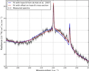
Fig. 7.Fits of a high latitude spectrum during winter. The black spec-trum was measured with FP1 at 89◦

N in March 2007. The blue and red lines indicate respectively the fits of this spectrum with the haze B cross-sections as measured byde Kok et al.(2007) and with the addi-tion of a small offset (2.5 cm−1_{) to haze B cross-sections from 190 cm}−1 to 240 cm−1_{. Without this correction, the continuum is overestimated} by NEMESIS around the C4H2 band and underestimated around the C2N2band.

without C4H2 (219−222 cm−1), C2N2 (233−236 cm−1), and

C3H4(322−334 cm−1). Then, we define the following domains

in regions of the spectra without strong emission lines around the retrieved gases:

– [214; 219[ ∪ ]222; 225] cm−1(around the C4H2band);

– [228.5; 233[ ∪ ]236; 241] cm−1_{(around the C}

2N2band);

– [317; 322[ ∪ ]334; 337] cm−1(around the C3H4band).

In each of these spectral domains, we estimate the new error bars σ with

σ = max (Imes− Icont)

with Imesthe measured radiance and Icontthe synthetic spectrum

of the continuum. We use σ as the new value of the minimum error in the whole domain (including the band of the considered gas).

3.4. Correction of the continuum at high latitudes during autumn and winter

We note that in several spectra acquired at high northern and southern latitudes (from 70◦N/S to 90◦N/S) during their respec-tive winter (2006−2007) and autumn (2014−2016), the con-tinuum component has a different shape in the 190−240 cm−1

range from that in the other spectra acquired at different lati-tudes or seasons. This shape is characterised by a broad emis-sion feature centred at 220 cm−1. Previous studies such as Coustenis et al. (1999), Anderson et al. (2012), Jennings et al. (2012, 2015) measured the same spectral feature in Voy-ager/IRIS and Cassini/CIRS data, at similar latitudes and sea-sons, and suggested that it could be caused by a mixture of ni-trile condensates. This new shape of the continuum could not be fitted correctly with temperature, and the cross-sections and ver-tical distributions measured for hazes 0 and B byde Kok et al. (2007,2010). For instance, in Fig.7, we compare the spectrum

measured at 89◦N in March 2007 and its fit by NEMESIS us-ing our nominal parameters for the hazes. Between 190 cm−1

and 222 cm−1, the radiance of the continuum of the mea-sured spectrum is lower than the radiance of the continuum fitted by NEMESIS, whereas there is the opposite situation from 222 cm−1 to 240 cm−1. Wavenumbers from 240 cm−1 to 400 cm−1 _{are not affected by this feature. This change in the}

continuum shape is an issue when trying to fit C4H2, C2N2, and

C3H4, as it affects the fits of C4H2 and C2N2 bands, and leads

to an underestimation of the abundance of C4H2and an

overes-timation of the abundance of C2N2.

However, we note that the continuum in the haystack re-gion (190−240 cm−1) can be fitted by adding a small offset in wavenumber to the cross-sections of haze B for the affected datasets. For the spectra measured at high northern latitudes during the winter (2006−2007), this offset is between 2 cm−1

and 2.5 cm−1, while its value is between 2.5 cm−1and 3 cm−1 for the observations of high southern latitudes during autumn (2012−2016). This offset would be consistent with the appear-ance of new condensates as suggested by the previous studies. The small difference between the offset values in the northern and southern high latitudes may be due to the fact that they were observed at different seasons (northern winter and southern au-tumn), and thus different stages of the chemical evolution at the poles.

3.5. Upper limits

For each FP1 dataset, we evaluate the level of detection of C4H2,

C2N2, and C3H4. For each gas, we define the χ2as

χ2₌ N X i=1 (Imes(wi) − Ifit(wi, x))2 2σ2 i , (2)

where Imes(wi) and Ifit(wi, x) are respectively the radiance

mea-sured at the wavenumber wiand the fitted radiance at the same

wavenumber for the volume mixing ratio x of the considered gas, N is the total number of points in the measured spectra, and σiis the error on the radiance measured at the wavenumber wi.

The factor 2 in the denominator is the oversampling factor of the data.

Then we compute the misfit∆χ2_{defined as}

∆χ2_{= χ}2_−χ2

0, (3)

where χ2

0 is the χ

2_{obtained when we fix the abundance of the}

considered gas to x= 0. The 1-σ, 2-σ, or 3-σ detection level is reached when∆χ2is respectively inferior to −1, −4, or −9. Most of the spectra acquired at high and mid-northern latitudes and at the south pole in autumn allow us to measure the abundances of C2N2, C3H4, and C4H2with a confidence level greater than 3-σ.

For some datasets, mostly the observations in the equatorial region, at southern mid-latitudes, and at southern high latitudes during summer, the signal-to-noise ratio is not good enough to detect the spectral bands of one or several of the studied species. For these datasets, for each undetected gas, we obtain an upper limit of its volume mixing ratio x by calculating synthetic spectra for different values of x, starting with x = 0 and incrementing it progressively. For each of these synthetic spectra, we compute the misfit∆χ2_{. The value of x for which∆χ}2_{is minimum is the}

upper limit for the volume mixing ratio of the considered gas. In these cases,∆χ2is positive and values of 1, 4, and 9 respectively indicate a 1-, 2-, or 3-σ upper limit.

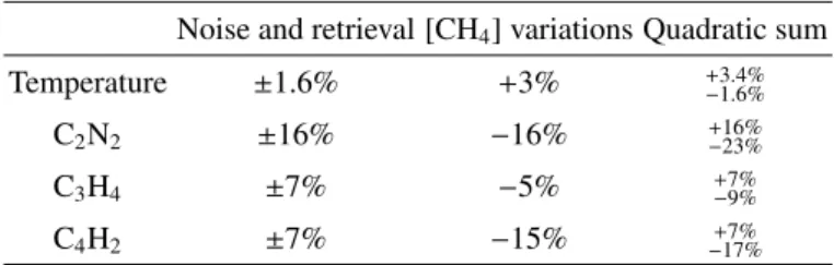
Table 2. Error estimation on the temperature and gases retrievals.

Noise and retrieval [CH4] variations Quadratic sum

Temperature ±1.6% +3% +3.4%_−1.6%

C2N2 ±16% −16% +16%−23%

C3H4 ±7% −5% +7%−9%

C4H2 ±7% −15% −17%+7%

3.6. Error analysis

Our retrievals are mainly affected by three error sources: mea-surement noise, errors related to the retrieval process (e.g. smoothing of the retrieved profile, forward modelling error), and the uncertainty on the CH4 abundance. The effects of the

first two error sources are directly estimated by NEMESIS. Lellouch et al.(2014) showed that at 15 mbar, CH4 abundance

varies from 1.0 to 1.5%. The upper value is consistent with the measurements from Niemann et al. (2010), which is the CH4abundance used in our reference atmosphere. We perform

additional retrievals to evaluate how a CH4abundance as low as

1.0% would affect our results. We find that the temperature re-trieved at 15 mbar would increase by 4−5 K (which is consistent with the results ofLellouch et al. 2014), and that the uncertainty on the CH4abundance is the dominant error source for the

tem-perature retrievals. This temtem-perature change would also decrease the retrieved volume mixing ratios of C2N2, C3H4, and C4H2.

For C2N2and C3H4, the difference between retrievals performed

with 1.0% and 1.48% of CH4 is comparable to the combined

effect of measurement noise and retrieval errors. For C4H2, the

effect of CH4 variation is twice as big as that of the other error

sources. These results are summarised in Table2.

4. Results

4.1. Radiance evolution at high latitudes

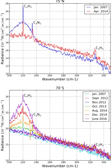
Figure8shows the spectra measured at 75◦N (top panel) in 2007 and 2014, and at 70◦S between 2007 and 2016. At both lati-tudes there is a striking evolution of the measured radiances as Titan’s atmosphere goes from northern winter to spring. Radi-ance variations of this amplitude are only observed at high north-ern and southnorth-ern latitudes. In both cases presented in Fig. 8, the largest change in the measured radiance occurs between 200 cm−1 and 250 cm−1. At 75◦N the broad emission feature centred on 220 cm−1_{present during northern winter (2007)}

com-pletely disappeared in mid-spring. The amplitude of the spectral bands of C4H2 (220 cm−1) and C2N2 (234 cm−1) slightly

de-creased from 2007 to 2014, but these bands are still clearly visi-ble in 2014.

At 70◦_{S, the temporal coverage of the data is better than at}

75◦N and allows us to follow more precisely the evolution of the radiance at this latitude. A broad emission feature centred at 220 cm−1, similar to what was observed at the northern high lat-itudes appeared in 2013 and its radiance increased steeply from October 2013 to June 2016, while radiances between 250 cm−1 and 400 cm−1_{(except in C}

3H4 band at 327 cm−1) stayed

con-stant during this period. The radiance in the broad emission fea-ture (except in C4H2 band) is higher at 70◦S in 2014 and 2016

(southern autumn) than at 75◦_{N in 2007 (northern winter). The}

radiance in the bands of C4H2(220 cm−1) and C2N2(234 cm−1)

M. Sylvestre et al.: Seasonal evolution of C2N2, C3H4, and C4H2 200 220 240 260 280 300 320 340

Wavenumber (cm-1)

Ra

dia

nc

e (

/

/

/

)

75

N

Wavenumber (cm-1)

Ra

dia

nc

e (

/

/

/

)

70

S

Fig. 8.Evolution of measured radiances at 75◦

N (top panel) and 70◦ S (bottom panel) from 2007 (northern winter) to 2016 (mid-spring). The sharp variation in the radiance between 228 cm−1_{and 231 cm}−1_{in the} spectra measured in August 2014 is a spurious noise feature which could not be eliminated during the calibration process. From 2007 to 2016, radiance at high southern latitudes has strongly increased, whereas it has decreased at high northern latitudes.

2007, the signal-to-noise ratio in the vicinity of the bands of C4H2 and C2N2 was too low to distinguish these spectral

fea-tures unambiguously. After September 2012, their radiances in-creased remarkably within a few months. The radiance of the C3H4 (327 cm−1) band also increased during the same period,

but more slowly than the other gases. The evolution of the radi-ances in the spectral bands of C4H2, C3H4, and C2N2 is faster

at 70◦S than at 75◦N. The changes in the radiances at 75◦N and 70◦_{S suggest a significant seasonal evolution of the lower}

strato-spheric composition.

4.2. Evolution of the meridional distributions of C4H2, C2N2,

and C3H4

Figure9shows the retrieved evolution of the meridional distri-butions of C4H2, C2N2, and C3H4from 2006 (northern winter)

to 2016 (late spring) at the 15 mbar pressure level (or an altitude of ∼85 km).

The most striking feature in the plots of Fig.9 is the sud-den and steep increase of the abundances of C4H2, C2N2, and

50 0 50 -90 -70 -30 -10 10 30 70 90

Latitude

Volume Mixing Ratio

C4H2 2004-2008 (a) 2004-2008 (FP3,b) 2009-2012 (FP3,c) 2010-2014 (FP3,d) 2006-2008 2009-2010 2012-2013 2014-2015 2016 50 0 50 -90 -70 -30 -10 10 30 70 90

Latitude

Volume Mixing Ratio

C2N2 2004-2008 (a) 2006-2008 2009-2010 2012-2013 2014-2015 2016 50 0 50 -90 -70 -30 -10 10 30 70 90

Latitude

Volume Mixing Ratio

C3H4 2004-2008 (a) 2004-2008 (FP3,b) 2009-2012 (FP3,c) 2010-2014 (FP3,d) 2006-2008 2009-2010 2012-2013 2014-2015 2016

Fig. 9.Meridional distributions of C4H2, C2N2, and C3H4 from 2006 (northern winter) to 2014 (mid-northern spring) at 15 mbar (or an altitude of ∼85 km). “a” refers to Teanby et al. (2009a), where the same gases as in this study were measured with the same CIRS de-tector (FP1); “b”, “c”, and “d” respectively refer to Coustenis et al.

(2010),Bampasidis et al.(2012), andCoustenis et al.(2016), C4H2and C3H4 were measured with the CIRS detector FP3, probing slightly higher pressure levels (10 mbar) than this study. In the south pole, from 2006 to 2015, the volume mixing ratios of the three species strongly increased, while the other latitudes exhibit weak seasonal vari-ations. Unlike C4H2 and C3H4, C2N2abundance at mid-northern lati-tudes decreases from 2012. Error bars show relative errors as derived in Sect.3.6.

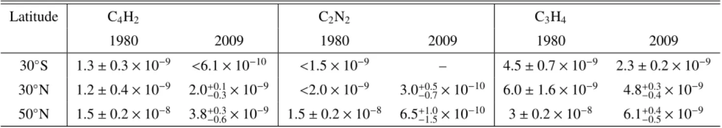
Table 3. Interannual comparison between abundances of C4H2, C2N2, and C3H4 measured by Voyager I/IRIS in November 1980 (Coustenis & Bezard 1995) and in this study in 2009.

Latitude C4H2 C2N2 C3H4 1980 2009 1980 2009 1980 2009 30◦_{S 1.3 ± 0.3 × 10}−9 _{<6.1 × 10}−10 _{<1.5 × 10}−9 _{– 4.5 ± 0.7 × 10}−9 _{2.3 ± 0.2 × 10}−9 30◦N 1.2 ± 0.4 × 10−9 2.0+0.1_−0.3× 10−9 <2.0 × 10−9 3.0+0.5_−0.7× 10−10 6.0 ± 1.6 × 10−9 4.8+0.3_−0.4× 10−9 50◦N 1.5 ± 0.2 × 10−8 3.8+0.3_−0.6× 10−9 _{1.5 ± 0.2 × 10}−8 _6.5+1.0 −1.5× 10 −10 _{3 ± 0.2 × 10}−8 _6.1+0.4 −0.5× 10 −9

C3H4 from 2006 to 2016 at high southern latitudes (poleward

of 70◦S). During this period, at 70◦S, abundances increased by at least a factor of 39 for C4H2, 39 for C2N2, and 10 for C3H4.

Most of this increase happened between 2012 and 2013. For in-stance, a factor of 2.4 can be measured between two consecutive measurements of C4H2volume mixing ratios at 70◦S during this

period.

In contrast, the other latitudes show smaller variations in the abundances of the studied gases. At high northern latitudes (poleward of 70◦_{N), the volume mixing ratios of C}

4H2, C2N2,

and C3H4have stayed constant from 2006 to 2015. In the

north-ern hemisphere, between 30◦_{N and 70}◦_{N, C}

3H4exhibits a di

ffer-ent seasonal evolution from C4H2and C2N2. Indeed, C3H4

abun-dance is constant from winter to late spring (from 2006 to 2016), whereas abundances of C4H2 and C2N2are constant from

win-ter to early spring (from 2006 to 2010), and then decrease in the middle of spring (after 2012). In equatorial and mid-southern latitudes (from 25◦N to 65◦S), C4H2 and C3H4volume mixing

ratios do not vary significantly from 2006 to 2015, then they in-crease in 2016 around 50◦S–60◦S. This evolution is sharp for C4H2(increasing by a factor 11) and weaker for C3H4

(increas-ing by a factor 2). For C2N2, there are fewer data points at

equa-torial and mid-southern latitudes because of the weaker signal-to-noise ratio in this band, but it seems to follow the same evo-lution as C3H4and C4H2.

The meridional distributions of the three gases follow the same trend in northern winter (2006−2008) and in early spring (2009−2010), with a decrease from the north pole to the south pole. This shape starts to evolve in mid-spring (2012) with the sudden enrichment in gases of the high southern latitudes. Then in late spring (2015−2016), the distributions of C2N2, C3H4, and

C4H2 at other latitudes slowly begin to evolve toward a more

symmetrical shape, with a decrease from poles to equator.

5. Discussion

5.1. Comparison with previous Cassini/CIRS measurements In Fig.9, our measurements are compared to the results from previous Cassini/CIRS observations of Titan’s lower strato-sphere. These abundances were inferred from

– nadir FP1 0.5 cm−1 _{resolution spectra (same type of data}

as in this study) fromTeanby et al.(2009a) during northern winter (2004−2008);

– nadir FP3 0.5 cm−1_{resolution spectra fromCoustenis et al.}

(2010) during northern winter (2004−2008), Bampasidis et al. (2012) during early northern spring (2009−2012), and Coustenis et al. (2016) during mid-northern spring (2010−2014).

Our results for the period 2006−2008 are in overall good agree-ment with the results of Teanby et al. (2009a). The C2N2 and

C3H4abundances measured in this study from 2006 to 2008 are

similar to the values of Teanby et al.(2009a). We find slightly lower C4H2abundances than they do, but this is probably due to

the update of the spectroscopic parameters for the C4H2band at

220 cm−1_{in GEISA 2015.}

The comparison between our results for C3H4and C4H2and

the FP3 measurements of Coustenis et al. (2010, 2016) and Bampasidis et al.(2012) shows that although we obtain values of the same order of magnitude, we often measure lower abun-dances. This is particularly visible on C3H4(at all seasons and

latitudes), whereas C4H2 abundances inferred in this study are

similar toCoustenis et al.(2010) in 2006–2008, then lower than Bampasidis et al.(2012) andCoustenis et al.(2016) after 2009. As these studies were performed in the 600−1100 cm−1region, C4H2and C3H4were not probed with the same spectral bands as

those in our study. This might be responsible for the small dis-parities between the results from nadir FP3 observations and this study. Differences between the retrieval codes (NEMESIS and ARTT) may also be at play. FP1 and FP3 results may also be dif-ferent because FP3 nadir observations probe slightly lower pres-sures (around 10 mbar or ∼100 km) than FP1 nadir observations (around 15 mbar or ∼85 km). This would be consistent with the predictions of photochemical models such as Wilson & Atreya (2004),Krasnopolsky(2014) andDobrijevic et al.(2016), where C3H4and C4H2profiles increase weakly with altitude in Titan’s

lower stratosphere.

5.2. Interannual variations

In Table3, we compare the results inferred from Voyager I/IRIS observations byCoustenis & Bezard(1995) with the abundances of C4H2, C3H4, and C2N2 measured with Cassini/CIRS in this

study. While we measure similar abundances at 30◦_{N, we}

ob-tain values slightly lower at 30◦S, and significantly lower at 50◦N than Coustenis & Bezard (1995). The largest difference between these two sets of measurements is reached for C2N2 at

50◦N: there is a factor of 23 difference between this study and the Voyager results. Coustenis et al.(2013) compared Voyager and Cassini/CIRS FP3 results and also found smaller C4H2and

C3H4abundances in 2009 than in 1980 at 50◦N. They suggested

that this could be due to variations of the solar activity, as 1980 observations occurred during a solar maximum. Our study shows that C2N2follows the same trend, which is consistent with this

explanation.

5.3. Influence of abundances at lower pressure levels on the nadir measurements

In this paper, we use uniform a priori profiles to retrieve C4H2,

C2N2, and C3H4. InVinatier et al.(2015), the authors measured

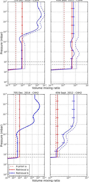
M. Sylvestre et al.: Seasonal evolution of C2N2, C3H4, and C4H2 10-10 ₁₀-9 ₁₀-8 ₁₀-7 ₁₀-6 ₁₀-5 10-5 10-4 10-3 10-2 10-1 100 101 102 103 70S Dec. 2014 - C3H4 10-10 ₁₀-9 ₁₀-8 ₁₀-7 45N Sept. 2012 - C3H4

Volume mixing ratio

Pressure (mbar)

Volume mixing ratio

Pressure (mbar)

Fig. 10.Vertical profiles of C3H4(top panels) and C4H2(bottom panels) retrieved at 70◦

S in December 2014 (left panels) and 45◦

N in September 2012 (right panels). Vertical profiles from retrievals (a) and their a pri-ori are respectively represented by red solid and dashed lines. Vertical profiles from retrievals (b) are represented by blue solid lines. A priori profiles for retrievals (b) are represented by blue dashed lines within the pressure range probed by the CIRS limb observations, and by blue dot-ted lines outside this pressure range. Thin black dashed lines show the pressure range probed by our CIRS nadir observations. The limb pro-files on the left and right panels (blue dashed lines) were respectively measured at 79◦

S in September 2014 and 46◦

N in June 2012. At the pressure levels probed by our observations, retrievals (a) and (b) give consistent results, except for C4H2at 70◦S in December 2014, because of the high vertical gradient of the a priori profile (b).

observations, and they showed that the vertical gradients of the abundance of these gases can be steep and exhibit strong tem-poral variations. In Fig. 10, we show two examples of vertical

profiles of C4H2 and C3H4 measured by Vinatier et al.(2015).

The abundances measured for these two gases at 79◦_{S in}

Septem-ber 2014 (blue dashed lines in the left panels) show a strong enrichment at low pressures (enrichment by a factor of 200 be-tween 0.1 mbar and 0.01 mbar), while much weaker vertical vari-ations were measured at 46◦N in 2012 (blue dashed lines in the right panels).

In order to evaluate how the shape of the vertical profiles of C3H4 and C4H2, and especially how an enrichment in these

species at high altitude can affect our results, we retrieve best-fitting scales factors for C3H4 and C4H2, using the limb

mea-surements fromVinatier et al.(2015) as a priori profiles. Above the upper sensitivity limit of the limb data, we use a constant ver-tical profile. Below the lower sensitivity limit of the limb data, we also set the profile to a constant value with pressure until we reach the condensation level, where the shape of the profile de-creases to mimic the condensation of the two considered species. We perform these retrievals for several nadir datasets ac-quired at several latitudes and seasons (72◦N in April 2007, 45◦_{N in September 2012, 75}◦_{N in April 2014, 70}◦_{S in December}

2014) using limb profiles measured at close latitudes and times (70◦_{N in August 2007, 46}◦_{N in June 2012, 71}◦_{N in January}

2015, 79◦S in September 2014). In the following paragraph, we discuss the effects of the C4H2 and C3H4 a priori profiles

with the largest and the smallest vertical gradients using two observations:

– the retrieval of the nadir data at 45◦_{N observed in September}

2012, using the limb profile measured at 46◦N in June 2012 as an a priori (low vertical gradients);

– the retrieval of the nadir data at 70◦_{S observed in December}

2014, using the limb profile measured at 79◦S in September 2014 as an a priori (high vertical gradients).

Figure 10shows the comparison between the results obtained using constant a priori profiles (retrievals (a)) and a priori profiles from the limb observations ofVinatier et al.(2015) (re-trievals (b)), for C4H2 and C3H4 for the selected examples.

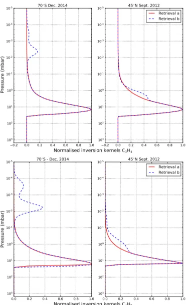
Figure 11 shows the inversion kernels obtained for C4H2 and

C3H4with the retrievals (a) and (b).

Low vertical gradient – 45◦_{N in September 2012}

When the vertical gradients in the a priori profiles of C4H2and

C3H4 are low, the inversion kernels of the retrievals (a) and

(b)are slightly different; the volume mixing ratios measured at higher altitude are large enough to broaden the base of the con-tribution functions. However, these variations of the contribu-tion funccontribu-tion are small compared to the size of its main lobe. This is consistent with the fact that the profiles obtained from retrievals (b) are within error bars from the profiles (a) at the pressure levels probed by nadir observations (from 18 mbar to 9 mbar). Above this pressure range, the difference between the profiles (a) and (b) is larger than the error bars because we re-trieve a scale factor of the a priori profiles.

High vertical gradient – 70◦_{S in December 2014}

When the vertical gradients of the a priori profiles of C3H4and

C4H2are high, a second lobe can appear in the contribution

func-tions. For C3H4, this second lobe is small compared to the main

lobe, which means that the enrichment in C3H4measured around

0.004 mbar does not affect the nadir measurements at 15 mbar. For C4H2, the second peak of the contribution function is not

0.2 0.0 0.2 0.4 0.6 0.8 1.0 10-5 10-4 10-3 10-2 10-1 100 101 102 103 Pressure (mbar) 70◦S Dec. 2014 0.2 0.0 0.2 0.4 0.6 0.8 1.0 10-5 10-4 10-3 10-2 10-1 100 101 102 103 45◦N Sept. 2012 Retrieval a Retrieval b

Normalised inversion kernels C3H4

0.0 0.2 0.4 0.6 0.8 1.0 10-5 10-4 10-3 10-2 10-1 100 101 102 103 Pressure (mbar) 70◦S - Dec. 2014 0.0 0.2 0.4 0.6 0.8 1.0 10-5 10-4 10-3 10-2 10-1 100 101 102 103 45◦N Sept. 2012 Retrieval a Retrieval b

Normalised inversion kernels C4H2

Fig. 11.Inversion kernels for retrievals a (red solid line) and b (blue dashed lines) for C3H4(top) and C4H2(bottom). They were calculated from the nadir retrievals performed with the observations at 70◦

S in De-cember 2014 (left panels) and 45◦

N in September 2012 (right panels). The vertical gradients of the a priori profiles can affect the shape of the contribution functions.

negligible compared to the main peak. As a result, the profile (b) is significantly lower than the profile (a) in the sensitivity range because of the contribution from high altitudes. There is a factor of 2.3 between these two profiles of C4H2, which is the greatest

difference found among the different datasets for which we per-formed these tests. Profiles (a) and (b) of C3H4are within error

bars. Thus, we can conclude that the abundances of C4H2from

the nadir measurements at high southern latitudes during autumn may be slightly overestimated, by less than a factor 2.3. How-ever, the relative abundances variations of C4H2remain robust.

5.4. Implications for photochemistry and atmospheric dynamics

The seasonal evolution of the abundances of the trace species is the result of a complex interplay between photochemistry and atmospheric dynamics. Measurements of the trace species dis-tribution at several latitudes and altitudes help to explain these different processes.

Global climate models (GCM; Hourdin et al. 1995;

Tokano et al. 1999; Lebonnois et al. 2012) predict that atmo-spheric circulation of Titan takes the form of a global cell with an upwelling branch above the summer pole and a subsiding branch above the winter pole. Around equinoxes, as the at-mospheric circulation is reversing, there are two Hadley cells with upwelling at the equator and subsidence above the poles. The seasonal evolution of the abundances of C4H2, C2N2, and

C3H4 at 15 mbar can be related to the effects of atmospheric

dynamics in the lower stratosphere. According to the predictions of the GCMs, high latitudes should be particularly sensitive to the seasonal changes, which is in good agreement with our observations at Titan’s south pole. Indeed, in Sect.4, we show that after 2012, during southern autumn, high southern latitudes exhibit a strong and sudden enrichment in C2N2, C4H2, and

C3H4. This is similar to what has been measured at higher

alti-tudes in the stratosphere by previous studies (Teanby et al. 2012; Vinatier et al. 2015;Coustenis et al. 2016). This enrichment has been interpreted as the effect of the subsiding branch of the Hadley cell above these latitudes, carrying these photochemical products from the upper stratosphere. Our measurements (see Fig. 9) show that this subsidence above the autumn pole also affects this part of the stratosphere, in good agreement with the atmospheric circulation predicted by the GCM of Lebonnois et al. (2012). In addition, in Teanby et al. (2012), Vinatier et al.(2015), the authors show that the enrichment in species such as HCN, C4H2, or C3H4 appeared in the upper

stratosphere at 500 km (0.001 mbar) between June and Septem-ber 2011, during southern autumn. As the 15 mbar pressure level (∼85 km of altitude) began to exhibit the same enrichment in C4H2, C3H4, and C2N2 between September and November

2012, we can infer that the air enriched in photochemical species has propagated toward the lower stratosphere in one year.

During winter, high northern latitudes were enriched in pho-tochemical species, and contrarily to the southern high latitudes, they exhibit stable abundances of C4H2, C2N2, and C3H4 from

northern winter to spring, similarly to what has been observed by Coustenis et al. (2016) for gases such as C4H2, C3H4, or

C6H6at 10 mbar. There is a strong difference between the

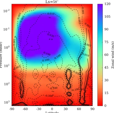
sea-sonal variations of these species at the probed pressure level (15 mbar) and the seasonal variations measured at lower pres-sures byVinatier et al.(2015). Indeed, they measured a strong enhancement of trace gases between 0.01 mbar and 0.001 mbar, after the equinox (in 2010), which disappeared one year later. Figure 12 shows the stream functions predicted by the GCM simulation fromLebonnois et al.(2012) during northern spring. Progressively, the circulation is evolving from two equator-to-pole cells to a single equator-to-pole-to-equator-to-pole cell (with upwelling above the north pole and downwelling above the south pole). Figure 12 shows that to reach this final state, the northern equator-to-pole cell shrinks in latitude and moves toward the north pole. This small cell may act like a “trap” for the photochemical species, keeping the amount of photochemical products constant near the north pole and preventing them from being advected toward the other latitudes by the bigger cell. The latitudinal extent of the small cell seems to vary with the pressure level: between 5 mbar and 11 mbar it extends from 60◦N and 85◦N, while it is very narrow at 0.1 mbar as it goes from 70◦_{N to 75}◦_{N. This di}

ffer-ence may explain why seasonal variations were measured at low pressures in limb measurements while abundances stay constant in our nadir measurements.

The seasonal evolution of the poles is also characterised by the strong radiance variations shown in Fig. 8, centred at 220 cm−1_{. Jennings et al. (2012, 2015) used Cassini/CIRS}

M. Sylvestre et al.: Seasonal evolution of C2N2, C3H4, and C4H2

Fig. 12. Zonal winds and stream function (109 _{kg/s) at L}

S = 58◦

(July 2014) from the numerical simulation inLebonnois et al.(2012). Solid and dashed lines indicate respectively clockwise and anticlock-wise rotation.

data to study this spectral feature and suggested (following Coustenis et al. 1999;de Kok et al. 2008;Anderson et al. 2012) that it is the signature of a cloud mainly composed of nitriles located between 80 km and 150 km.Jennings et al.(2012) sug-gested that the disappearance of this cloud above the north pole could be related to the increase in insolation at these latitudes which would lead to more photolysis of the source chemicals of this cloud at higher altitudes, and to a lessening of condensa-tion, or to a weakening of the subsiding branch above the north pole. However, during spring, abundances of various gases have stayed constant (in this study and in Coustenis et al. 2016) in the lower stratosphere above high northern latitudes. This would imply that the disappearance of the cloud is more related to the seasonal insolation variations than to dynamics. Above the south pole, we show that the emission at 220 cm−1 _{has kept}

on increasing in 2014 and 2016, which is quite surprising as Jennings et al.(2015) suggested that a decrease in the radiances at these latitudes should occur in 2015−2016, based on north pole behaviour.

In this study, we find that meridional distributions of C4H2and C3H4do not evolve between 50◦S and 30◦N from 2006

to 2015. This is compatible with the results ofBampasidis et al. (2012), where the distributions of these gases were measured from 2006 to 2012. Bampasidis et al. (2012) also monitored sharp variations in C3H4 and C4H2 (and other gases such as

C2H4or HCN) between 2008 and 2010, characterised by a steep

increase until mid-2009 and then a decrease in their abundances. They attributed this evolution to the rapid changes in atmo-spheric circulation around equinox, and especially the weaken-ing of the vortex observed in the northern winter hemisphere. These temporal variations are not present in our data. It may be because we do not have enough data at 50◦N in 2009−2010. It might also indicate that unlike higher pressure levels, the atmo-spheric circulation at 15 mbar does not exhibit sharp changes around the equinox, and evolves more steadily.

Photochemistry also controls the distribution of trace gases in the stratosphere. In Fig. 9, we show that at mid-northern latitudes C3H4 abundances are constant, while C2N2 and

C4H2 abundances decrease in 2014−2016. The photochemical

model ofLavvas et al.(2008) predicts that C4H2photochemical

lifetime at 150 km (2 mbar) is 0.2 yr, which is 10 times lower than for C3H4(2 yr). If there is a similar difference between the

photochemical lifetimes of these two species at 15 mbar, this can explain why a diminution of C4H2abundances is observed, while

C3H4abundances do not vary. As C2N2follows the same trend

as C4H2, this would suggest that C2N2and C4H2photochemical

lifetimes at 15 mbar are of the same order of magnitude. Photochemical models disagree on the loss mechanisms of these species. In the photochemical model of Titan’s atmosphere presented byKrasnopolsky(2014), photolysis is the major sink for C2N2(68% of loss), whereas it is a minor loss mechanism for

C4H2 and C3H4 (7% and 9% of loss respectively). This would

mean that C2N2 could be more sensitive than C4H2 to the

sea-sonal variations of insolation, which is not consistent with our results. However, in the photochemical model ofVuitton et al. (2014), photolysis is a minor loss reaction for the three studied species at the probed pressure-level. Their main loss reaction is the combination with atomic hydrogen, for instance,

C4H2+ H → C4H3+ hν,

which would be consistent with the fact that C2N2and C4H2vary

in a similar way in the northern hemisphere during spring.

6. Conclusion

In this work, we study the seasonal evolution of Titan’s lower stratosphere, using Cassini/CIRS far-infrared observa-tions. These data allow us to probe the atmosphere around the 15 mbar pressure level and to measure the abundances of three photochemical by-products: C2N2, C3H4, and C4H2. Thanks to

the long duration of the Cassini mission and the good latitudinal coverage of these data, we have been able to monitor the evolu-tion of these species over the whole latitude range from 2006 to 2016, i.e. from northern winter to mid-spring.

The most striking feature is the asymmetry in the seasonal evolution of high northern latitudes where the volume mixing ratios of C4H2, C2N2, and C3H4 have stayed approximately

constant from northern winter to spring, whereas high south-ern latitudes exhibit a sudden and strong enrichment in these species during southern autumn, consistent with the observa-tions at 10 mbar ofCoustenis et al.(2016). We also show that C3H4has a different seasonal evolution compared to C2N2 and

C4H2 at mid-northern latitudes, which may be due to shorter

photochemical lifetimes for the two latter species.

The evolution of the high latitudes is consistent with the sea-sonal evolution of Titan’s atmospheric circulation predicted by the GCM ofLebonnois et al.(2012) as the effect of a subsidence above the south pole and the presence of a small circulation cell towards the high northern latitudes can explain our results.

Acknowledgements. The authors thank Véronique Vuitton for very useful dis-cussions about Titan’s photochemistry and Emmanuel Lellouch for his com-ments about possible effects of high altitudes abundances on our retrievals. We also thank the anonymous reviewer for the suggestions that improved this pa-per. This research was funded by the UK Sciences and Technology Facilities Research council (grant number ST/MOO7715/1) and the Cassini project.

References

Achterberg, R. K., Conrath, B. J., Gierasch, P. J., Flasar, F. M., & Nixon, C. A. 2008,Icarus, 194, 263

Anderson, C., Samuelson, R., & Achterberg, R. 2012, in Titan Through Time, Unlocking Titan’s Past, Present and Future, eds. V. Cottini, C. Nixon, & R. Lorenz, 59

Bampasidis, G., Coustenis, A., Achterberg, R. K., et al. 2012,ApJ, 760, 144

Borysow, A. 1991,Icarus, 92, 273

Borysow, A., & Frommhold, L. 1986a,ApJ, 311, 1043

Borysow, A., & Frommhold, L. 1986b,ApJ, 303, 495

Borysow, A., & Frommhold, L. 1986c,ApJ, 304, 849

Borysow, A., & Frommhold, L. 1987,ApJ, 318, 940

Borysow, A., & Tang, C. 1993,Icarus, 105, 175

Cottini, V., Nixon, C. A., Jennings, D. E., et al. 2012,Icarus, 220, 855

Coustenis, A., & Bezard, B. 1995,Icarus, 115, 126

Coustenis, A., Bezard, B., Gautier, D., Marten, A., & Samuelson, R. 1991,

Icarus, 89, 152

Coustenis, A., Schmitt, B., Khanna, R. K., & Trotta, F. 1999,Planet. Space Sci., 47, 1305

Coustenis, A., Achterberg, R. K., Conrath, B. J., et al. 2007,Icarus, 189, 35

Coustenis, A., Jennings, D. E., Nixon, C. A., et al. 2010,Icarus, 207, 461

Coustenis, A., Bampasidis, G., Achterberg, R. K., et al. 2013,ApJ, 779, 177

Coustenis, A., Jennings, D. E., Achterberg, R. K., et al. 2016,Icarus, 270, 409

de Kok, R., Irwin, P. G. J., Teanby, N. A., et al. 2007,Icarus, 191, 223

de Kok, R., Irwin, P. G. J., & Teanby, N. A. 2008,Icarus, 197, 572

de Kok, R., Irwin, P. G. J., & Teanby, N. A. 2010,Icarus, 209, 854

Dobrijevic, M., Loison, J. C., Hickson, K. M., & Gronoff, G. 2016,Icarus, 268, 313

Flasar, F. M., Kunde, V. G., Abbas, M. M., et al. 2004,Space Sci. Rev., 115, 169

Hanel, R., Conrath, B., Flasar, F. M., et al. 1981,Science, 212, 192

Hourdin, F., Talagrand, O., Sadourny, R., et al. 1995,Icarus, 117, 358

Irwin, P. G. J., Teanby, N. A., de Kok, R., et al. 2008,J. Quant. Spectr. Rad. Transf., 109, 1136

Jacquinet-Husson, N., Armante, R., Scott, N. A., et al. 2016,J. Mol. Spectr., 327, 31

Jennings, D. E., Anderson, C. M., Samuelson, R. E., et al. 2012,ApJ, 754, L3

Jennings, D. E., Achterberg, R. K., Cottini, V., et al. 2015,ApJ, 804, L34

Krasnopolsky, V. A. 2014,Icarus, 236, 83

Kunde, V. G., Aikin, A. C., Hanel, R. A., et al. 1981,Nature, 292, 686

Lavvas, P. P., Coustenis, A., & Vardavas, I. M. 2008,Planet. Space Sci., 56, 27

Lebonnois, S., Burgalat, J., Rannou, P., & Charnay, B. 2012,Icarus, 218, 707

Lellouch, E., Bézard, B., Flasar, F. M., et al. 2014,Icarus, 231, 323

Maltagliati, L., Bézard, B., Vinatier, S., et al. 2015,Icarus, 248, 1

Molter, E. M., Nixon, C. A., Cordiner, M. A., et al. 2016,AJ, 152, 42

Niemann, H. B., Atreya, S. K., Demick, J. E., et al. 2010,J. Geophys. Res. (Planets), 115, E12006

Nixon, C. A., Temelso, B., Vinatier, S., et al. 2012,ApJ, 749, 159

Teanby, N. A., de Kok, R., Irwin, P. G. J., et al. 2008a,J. Geophys. Res. (Planets), 113, E12003

Teanby, N. A., Irwin, P. G. J., de Kok, R., et al. 2008b,Icarus, 193, 595

Teanby, N. A., Irwin, P. G. J., de Kok, R., et al. 2009a,Icarus, 202, 620

Teanby, N. A., Irwin, P. G. J., de Kok, R., & Nixon, C. A. 2009b,Phil. Trans. Roy. Soc. London Ser. A, 367, 697

Teanby, N. A., Irwin, P. G. J., Nixon, C. A., et al. 2012,Nature, 491, 732

Tokano, T., Neubauer, F. M., Laube, M., & McKay, C. P. 1999,

Planet. Space Sci., 47, 493

Tomasko, M. G., Bézard, B., Doose, L., et al. 2008a,Planet. Space Sci., 56, 648

Tomasko, M. G., Doose, L., Engel, S., et al. 2008b,Planet. Space Sci., 56, 669

Vinatier, S., Bézard, B., Nixon, C. A., et al. 2010,Icarus, 205, 559

Vinatier, S., Rannou, P., Anderson, C. M., et al. 2012,Icarus, 219, 5

Vinatier, S., Bézard, B., Lebonnois, S., et al. 2015,Icarus, 250, 95

Vuitton, V., Dutuit, O., Smith, M. A., & Balucani, N. 2012, in Titan: Interior, Surface, Atmosphere, and Space Environment, eds. I. Müller-Wodarg, C. A. Griffith, E. Lellouch, & T. E. Cravens (Cambridge: Cambridge University Press), 224

Vuitton, V., Yelle, R. V., Klippenstein, S. J., Hörst, S. M., & Lavvas, P. 2014, in AAS/Division for Planetary Sciences Meeting Abstracts, 46, 105.01 Wilson, E. H., & Atreya, S. K. 2004,J. Geophys. Res. (Planets), 109, E06002

M. Sylvestre et al.: Seasonal evolution of C2N2, C3H4, and C4H2

Appendix A

Table A.1. Datasets used in this study.

Observations Date N FP1 Lat. FP1(◦N) FOV FP1(◦) N FP4 Lat. FP4(◦N)

CIRS_036TI_FIRNADCMP002_PRIME* 28 Dec. 2006 136 –89.1 12.6 684 –74.2 CIRS_036TI_FIRNADCMP003_PRIME*† 27 Dec. 2006 321 78.6 21.0 1620 74.2 CIRS_037TI_FIRNADCMP001_PRIME† 12 Jan. 2007 161 75.2 19.1 815 83.3 CIRS_037TI_FIRNADCMP002_PRIME 13 Jan. 2007 107 –70.3 20.6 540 –84.2 CIRS_038TI_FIRNADCMP001_PRIME† 28 Jan. 2007 254 86.3 16.7 1275 69.0 CIRS_040TI_FIRNADCMP001_PRIME* 09 Mar. 2007 159 –49.2 21.1 795 –61.2 CIRS_040TI_FIRNADCMP002_PRIME*† 10 Mar. 2007 109 88.8 13.3 545 69.0 CIRS_041TI_FIRNADCMP002_PRIME* 26 Mar. 2007 102 61.2 19.3 525 47.9 CIRS_042TI_FIRNADCMP002_PRIME* 11 Apr. 2007 272 71.5 22.6 1362 50.6 CIRS_043TI_FIRNADCMP002_PRIME*† 27 Apr. 2007 104 77.1 20.0 535 55.0 CIRS_044TI_FIRNADCMP002_PRIME* 13 May 2007 104 –0.5 18.8 524 –17.3 CIRS_045TI_FIRNADCMP002_PRIME* 29 May 2007 346 52.4 29.5 1735 30.0 CIRS_046TI_FIRNADCMP002_PRIME 14 Jun. 2007 102 –20.8 19.0 510 –38.3 CIRS_052TI_FIRNADCMP002_PRIME* 19 Nov. 2007 272 40.3 26.5 1365 19.3 CIRS_053TI_FIRNADCMP001_PRIME* 04 Dec. 2007 223 –40.2 25.8 1119 –49.8 CIRS_055TI_FIRNADCMP001_PRIME 05 Jan. 2008 190 18.7 30.5 960 5.6 CIRS_055TI_FIRNADCMP002_PRIME 06 Jan. 2008 284 44.6 22.2 1420 39.9 CIRS_069TI_FIRNADCMP002_PRIME* 28 May 2008 112 9.5 19.3 565 –9.2 CIRS_107TI_FIRNADCMP002_PRIME 27 Mar. 2009 164 33.5 30.4 821 50.1 CIRS_110TI_FIRNADCMP001_PRIME 06 May 2009 282 –68.1 25.7 1410 –59.4 CIRS_111TI_FIRNADCMP002_PRIME 22 May 2009 168 –27.1 23.1 842 –21.6 CIRS_112TI_FIRNADCMP001_PRIME 06 Jun. 2009 218 48.7 21.0 1090 59.0 CIRS_112TI_FIRNADCMP002_PRIME 07 Jun. 2009 274 –58.9 20.2 1370 –39.9 CIRS_160TI_FIRNADCMP002_PRIME 30 Jan. 2012 280 –0.2 18.3 1474 6.9 CIRS_172TI_FIRNADCMP001_PRIME 26 Sep. 2012 282 44.9 18.5 1410 50.9 CIRS_172TI_FIRNADCMP002_PRIME† 26 Sep. 2012 270 –70.4 23.2 1352 –70.8 CIRS_174TI_FIRNADCMP002_PRIME 13 Nov. 2012 298 –71.8 21.8 1493 –52.9 CIRS_194TI_FIRNADCMP001_PRIME 10 Jul. 2013 186 30.0 19.7 935 46.1 CIRS_197TI_FIRNADCMP001_PRIME 11 Sep. 2013 330 60.5 19.4 1650 64.0 CIRS_198TI_FIRNADCMP001_PRIME 13 Oct. 2013 187 88.9 8.7 935 72.9 CIRS_198TI_FIRNADCMP002_PRIME† 14 Oct. 2013 306 –69.8 24.0 1530 –85.8 CIRS_199TI_FIRNADCMP001_PRIME 30 Nov. 2013 329 68.4 23.9 1650 85.5 CIRS_200TI_FIRNADCMP001_PRIME 01 Jan. 2014 187 49.9 19.6 935 37.2 CIRS_201TI_FIRNADCMP001_PRIME 02 Feb. 2014 329 19.9 26.8 1649 27.6 CIRS_203TI_FIRNADCMP001_PRIME 07 Apr. 2014 187 75.0 18.0 935 67.7 CIRS_207TI_FIRNADCMP001_PRIME† 20 Aug. 2014 179 –70.0 17.8 895 –79.4 CIRS_207TI_FIRNADCMP002_PRIME 21 Aug. 2014 39 79.8 16.1 195 78.1 CIRS_208TI_FIRNADCMP002_PRIME 22 Sep. 2014 175 60.5 17.8 875 75.6 CIRS_210TI_FIRNADCMP001_PRIME† 10 Dec. 2014 329 –70.3 25.5 1646 –50.5 CIRS_218TI_FIRNADCMP001_PRIME 06 Jul. 2015 249 –20.0 19.9 1250 –2.9 CIRS_222TI_FIRNADCMP002_PRIME 29 Sep. 2015 233 –0.1 18.6 530 18.3 CIRS_232TI_FIRNADCMP001_PRIME 16 Feb. 2016 249 –50.2 24.5 1245 –31.0 CIRS_235TI_FIRNADCMP001_PRIME† 06 May 2016 163 –60.0 19.7 820 –45.1 CIRS_236TI_FIRNADCMP001_PRIME † 07 Jun. 2016 88 –70.0 15.8 440 –53.2 CIRS_236TI_FIRNADCMP002_PRIME 07 Jun. 2016 238 60.0 19.8 1193 78.7

Notes. N FP1 and N FP4 respectively stand for the number of spectra measured with FP1 and FP4 during the acquisition. FOV is the field of view. The asterisk denotes the datasets which have already been presented inTeanby et al.(2009a). The symbol † denotes datasets for which we perform the retrievals using small domains around the spectral bands of C4H2, C2N2, and C3H4, as described in Sect.3.4.