Designing structures with tree forks : mechanical characterization and generalized computational design approach

(1)

Designing structures with tree forks: Mechanical characterization

and generalized computational design approach

by Ishani Desai

B.S. in Civil and Environmental Engineering, Rice University, 2019 Massachusetts Institute of Technology, 2020

Submitted to the Department of Civil and Environmental Engineering in Partial Fulfillment of the Requirements for the degree of

MASTER OF ENGINEERING IN CIVIL AND ENVIRONMENTAL ENGINEERING

at the

MASSACHUSETTS INSTITUTE OF TECHNOLOGY May 2020

The author hereby grants to MIT permission to reproduce and to distribute publicly paper and electronic copies of this thesis document in whole or in part in any medium now known or hereafter created.

Signature of Author:

Ishani Desai Department of Civil and Environmental Engineering May 8, 2020 Certified by:

Caitlin Mueller Associate Professor, Civil and Environmental Engineering and Architecture Thesis Supervisor Accepted by:

Colette L. Heald Professor of Civil and Environmental Engineering Chair, Graduate Program Committee

(2)

Designing structures with tree forks: Mechanical characterization

and generalized computational design approach

by Ishani Desai

Submitted to the Department of Civil and Environmental Engineering on May 8, 2020 in Partial Fulfillment of the Requirements for the Degree of Master of Engineering in Civil and

Environment Engineering

ABSTRACT

Timber structures have seen a resurgence in structural design in recent years due to a desire to reduce embodied carbon in the built environment. While many of these structures use standardized or regular elements, the recent revolution in digital fabrication has resulted in a variety of more complex and irregular timber forms, usually achieved through milling or other machine-driven production processes. However, the organic nature of wood has also inspired architects and engineers to harness naturally occurring formal variation, for example, in the geometries of tree forks and branches, to produce designs that are more directly responsive to their constitutive materials. Compared to conventional fabrication processes for timber, in which the material is often processed several times to achieve characteristics that are present in the original material, this approach embodies little waste in material and effort.

Naturally occurring branching tree forks seem to exhibit outstanding strength and material efficiency as a natural moment connection, which underpins previous research investigating their use in design. This thesis advances the use of tree forks as a natural connection in structures through two specific contributions. First, the paper establishes a flexible matching-based methodology for designing structures with a pre-existing library of tree fork nodes (based on actual available materials from salvaged trees, for example), balancing an initial target design, node matching quality, and structural performance. The methodology uses a combination of Iterative Closest Point and Hungarian Algorithms as a real-time computational approach for matching nodes in the library to nodes in the design. The thesis presents results that systematically test this methodology by studying how matching quality varies depending on the number and species of tree forks available in the library and relates this back to the mechanical properties of tree branches found through physical testing.

Second, mechanical laboratory testing of tree fork nodes of various tree species (available locally in the area) is presented to quantify the structural capacity of these connections and observe the behavior under tree fork load transfers. A structural score is developed to characterize the tolerance of tree fork nodes to imperfect matches in terms of structural capacity; these resulting geometries are compared to the previous matching-based scoring system. The resulting approach is projected forward as a framework for a more general computational approach for designing with existing material systems and geometries that can also be expanded beyond tree forks.

Thesis Supervisor: Caitlin Mueller

(3)

(4)

ACKNOWLEDGMENTS

I would first like to thank my thesis advisor and professor, Caitlin Mueller, for her invaluable support throughout this academic year. I am continuously inspired by the work she leads within the Digital Structures group and always leave inspired about the progress and future of structural engineering after any meeting, discussion, or class.

I wish to acknowledge Felix Amtsberg, Kevin Moreno Gata, and Yijiang Huang for their previous work on this project as well. Their contributions instigated this project and provided much of the initial framework for the matching-based design algorithm.

I would also like to thank Christopher Dewart and Stephen Rudolph for their expertise and support in executing the structural capacity testing within the N51 Wood Shop and Pierce Laboratory.

I am forever thankful to my friends of the Master of Engineering program that made this year an unforgettable experience that went above and beyond my expectation.

Finally, I would like to thank my parents and my partner for their unconditional love and support during this year.

(5)

LIST OF FIGURES

Figure 1. Forced curvature in timber through cambering (Daizen Joinery) ... 14

Figure 2. “Natural” timber structure, Centre Pompidou Metz (Shigeru Ban Architects) ... 14

Figure 3. Diagram representation of oak trees as compass ship timbers (Albion 1926, 3) ... 15

Figure 4. Cross section of a ship ... 15

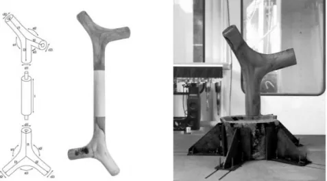
Figure 5. Tensile tree fork (left, Fig. 1) vs. Compression tree fork (right, Fig. 2) ... 16

Figure 6. Arrows show the direction of tree fork trunk fibers (TF), branch fibers (BF), and their intersection at the compaction zone (CZ) (Farrell 7) ... 17

Figure 7. Adaptive growth shown in the cross-section of a tree branch ... 18

Figure 8. Plan view of truss with mapped placement of tree forks... 19

Figure 9. Wood Chip Barn arching truss, completed (Mollica and Self 2016, 140) ... 19

Figure 10. Connection principle resulting in bifurcating space loops ... 20

Figure 11. Spatial geometries simulated to align branches with adjacent branch axis with Karamba loadings (Allner and Kroehnert 2018, 4) ... 20

Figure 12. Standard set of tree fork elements components and assembled (left). Processed and milled tree fork (right). (Von Buelow, Peter, et al. 2018, 2) ... 20

Figure 13. The basic ParaGen cycle showing the steps used to generate a range of solutions (Von Buelow, Peter, et al. 2018, 5) ... 21

Figure 14. Bridge truss system – ground structure (Brütting et al. 2018, 18) ... 22

Figure 15. Bridge truss – optimization results final topologies (Brütting et al. 2018, 20) ... 22

Figure 16. Bridge truss – assignment optimization (Brütting et al. 2018, 19) ... 23 Figure 17. Iterative form-finding process for inventory constrained design: a) parametrically

(8)

order by length, c) inventory elements pre-sorted in ascending order by length (Bakauskas et al.

2018, 8) ... 24

Figure 18. Process of acquiring material, digitizing inventory, designing and fabricating (Amtsberg et al.) ... 27

Figure 19. Tree forks collected and scanned from Somerville site (Amtsberg et al.) ... 27

Figure 20. Iterative Closest Point (ICP) and Hungarian algorithm matching tree fork material library to given structure (Huang et al.) ... 28

Figure 21. Prototype structure (Amtsberg et al.) ... 28

Figure 22. TreeKeeper database cataloguing all trees in Somerville, MA (“TreeKeeper”) ... 29

Figure 23. Visualizations of tree image generation data based on collected branching angles (Aono and Kunii 1984, 15) ... 30

Figure 24. (Left) Model of tree branching. (Middle) Tree skeleton with equivalent diameters for all branches. (Right) Tree skeleton utilizing Leonardo da Vinci’s rule. (Eloy) ... 30

Figure 25. Grasshopper sampling methodology visualization ... 31

Figure 26. Line representations of tree forks ... 32

Figure 27. Brep pipe representations of tree forks ... 32

Figure 28. Oak. 4x7: Hexagonal, 1 Control Curve. 100 samples. ... 35

Figure 29. Pavilion geometry with 2 control curves ... 36

Figure 30. Potential geometry given x, y, z-coordinate variables for each node ... 37

Figure 31. Hexagonal surface geometry generation process ... 38

Figure 32. 3 NURBS curves forming hexagonal grid surface ... 39

Figure 33. Height of lofted curve vs. degree of curvature geometry representation with constant curve angular x-rotation ... 40

(9)

Figure 34. Curve angular x-rotation vs. degree of curvature geometry representation with constant

height of lofted curve ... 40

Figure 35. Original pavilion geometry Matching Score vs. # of Samples ... 42

Figure 36. Matching score vs. Ratio (# of Structural Nodes : # of Samples). Worst performing geometries shown with bold lines: 3x3, 4x3, 5x3, 5x4, 6x3, 6x4, 6x5, 7x3, 7x4, 7x5, 7x6 ... 45

Figure 37. Boxed results represent the best matching scores for ash, oak, and fruit (cont.) ... 47

Figure 38. Example geometries for ash, oak, and fruit species that represent optimal matches (cont.) ... 48

Figure 39. Hexagonal geometry with 1 control curve, 4x3 & 5x5, homogenous geometries ... 49

Figure 40. Hexagonal geometry with 1 control curve, 3x7, variant geometries ... 50

Figure 41. Breaking modes: flat-surface (top right), imbedded-branch (top left), and ball-in-socket (bottom) (Farrell 2003, 37) ... 55

Figure 42. Typical moisture-strength properties of a red spruce (Wilson 1932) ... 56

Figure 43. a) Brep of tree scan, b) plane top/bottom, c) Prototrak top/bottom flat, d) plane 3rd edge, e) Joiner 3rd edge flat... 57

Figure 44. Fruit tree pre-processed fork ... 58

Figure 45. Ash tree pre-processed fork ... 58

Figure 46. Fruit tree control cube ... 59

Figure 47. Ash tree control cube ... 59

Figure 48. Fruit (top) and ash (bottom) tree fork setup – planed top forks sits at the center of the compression ... 60

Figure 49. Cube setup -- strain gauge attached ... 61

(10)

Figure 51. Fruit tree post-testing ... 62

Figure 52. Fruit tree fork testing results: Force vs. Displacement ... 63

Figure 53. Fruit tree cube testing results: Stress vs. Strain ... 63

Figure 54. Ash tree post-testing ... 64

Figure 55. Ash tree fork testing results: Force vs. Displacement ... 65

Figure 56. Ash tree cube testing results: Stress vs. Strain ... 65

Figure 57. Tree fork computational model mesh and point ... 67

Figure 58. Tree fork computational model reactions and principal stresses ... 68

Figure 59. Modeled center corresponding to the natural fibers of the tree fork ... 68

Figure 60. Angle difference between matched node and structural node ... 70

Figure 61. Hankinson equation graphical representation. N/P vs. Angle (“Wood Handbook”) .. 71

Figure 62. Ash. 3x4: Hexagonal, 1 Control Curve. 200 samples. ... 74

(11)

LIST OF TABLES

Table 1. Tree fork average, minimum, and maximum angles ... 30

Table 2. Ash, oak, and fruit tree branch angles ... 36

Table 3. Optimized pavilion geometry sampling matching score results ... 42

Table 4. Percent difference between structural testing and Wood Handbook of σcomp,|| & E... 66

(12)

(13)

1 Introduction & Literature Review

1.1 Background

While timber structures have seen a resurgence in structural engineering design, the complex structures built tend to disregard the inherent geometric advantages that the wood material contributes. Typically, the organic shapes desired are formed during post-processing of homogenized timber sections through either forced cambering or subtractive fabrication. A wasteful redundancy becomes apparent in which the material is processed several times to achieve characteristics that are present in the original material. Naturally occurring branching tree forks exhibit outstanding strength and material efficiency and are able to sustain a significant amount of structural load as a natural moment connection. The presented project investigates the feasibility of using tree forks as a natural design connection in structural frameworks. This will be conducted through a series of structural capacity testing as well as through sampling of tree fork nodes of various tree species found at a specific site location to form a digital material library.

1.2 Motivation

Utilization of natural grain patterns within trees was readily utilized centuries ago when timber was a more common construction material, specifically Dutch-era shipbuilding practices valued the natural efficiency of complex timber shapes (Albion 1926). However, as design materials shifted to concreate and steel, the perceived abundance and standardization of shapes dissolved the need and practice of harnessing the natural efficiency of timber. The expert skill shipbuilders possessed to select a tree by visually determining the availability of a specific shape needed for the design rather than either inducing a “needle-in-the-haystack” approach for finding a specific

(14)

member shape or using an immense amount of labor to form a highly specified member. The practice of utilizing the inherent strength of timber members was not only more labor efficient for shipbuilders, but also created stronger vessels since the wood grain in the pieces used aligned to their desired shape naturally (Gomes, Rosa Varela, et al. 2015). Unfortunately, this workflow has been lost with time, and desirable, “natural,” tree-looking structures are now most commonly produced through forcing curvature or aggressive postprocessing, as seen in Figure 1 and Figure 2. Therefore, one of the goals in this project is to revisit this idea of using the natural grain flow of trees to make a stronger, stiffer structure limiting unnecessary labor costs.

Figure 1. Forced curvature in timber through cambering (Daizen Joinery)

Figure 2. “Natural” timber structure, Centre Pompidou Metz (Shigeru Ban Architects) This project uses Somerville, Massachusetts as the location of its case studies, due to the availability of extracted trees in the area. The city has been engaging in controlled removals of urban trees as a nature preservation precaution to limit the expansion of an invasive beetle infestation (“Emerald Ash Borer Beetle” 2018) as well as a construction need clear land area for new developments. Instead of processing the trees in a woodchipper for alternate uses, the timber is collected and cut into viable tree fork nodes to be tested and analyzed for this thesis. The goal is to find a methodology to reuse the tree forks and branches in a way that could not only contribute to the community and area that the trees were cut down from but also develop a more general framework to be able to design with existing material systems and geometries. The trees were originally removed with the intention of designing a pavilion using the tree forks of the cut trees, so the target geometries proposed represent this utility. To limit the scope of the design, only the tree forks as connection joints and not the tree branches as beam elements will be considered in the design.

1.3 Literature review

This chapter reviews previous research and usage of natural forms of timber in structural design.

The first section discusses previous utilization of natural wood grains as “compass” timbers in

shipbuilding, the second section overviews the basic biomechanics of tree joints, the third section reviews several case studies that have utilized repurposed tree forks and branches architecturally, structurally, or computationally, and the fourth section details various instances of designing with existing materials. While there has been previous work regarding highly specific instances of tree fork utilization in structures, there has yet to be a comprehensive methodology of constructing a large material library and understanding of the structural behavior of a tree fork.

(15)

1.3.1 Shipbuilding with “compass” timbers

During the fifteenth century, timber was an essential resource for European countries, particularly the Netherlands, providing fuel, transportation, building material, and more. It was in the

countries’ strategic interests to take part in forest management and smart use of the limited

resource; otherwise, overuse would result in early-stage deforestation, which would be detrimental to the growth of the country. Shipbuilders offered a creative solution by being more mindful of the shape, potential placement, and usage of branches and bifurcations in the ship before cutting a tree down. To find the needed timber pieces, known as compass timbers, with the natural grain, the skilled master carpenter would have to have in his mind a clear view of what shapes were needed within the ship. The compass timbers and their intended placement within a ship are seen in Figure 3 and Figure 4. This approach of utilizing the natural shapes found in trees not only reduced material waste, but also creating the most structurally efficient ship (Albion 1926).

Figure 3. Diagram representation of oak trees as compass ship timbers (Albion 1926, 3)

Figure 4. Cross section of a ship (Albion 1926, 4)

Additional factors that contributed to the shipbuilders’ careful tree selection include: age, moisture content, and imperfections (knots). Each of these attributes affects the structural performance of the timber differently, so a thorough understanding of their implications by the shipbuilders was necessary to avoid complications within the built ship. For example, knots represent weak points in the timber structure, because it interrupts the natural grain of the trunk or branch and, with large loads, the timber may generate cracks or even worse, have a sudden failure. However, there is no such things as a perfect tree to convert to perfect timbers. The shipbuilders needed to know how to find the available raw material with an appropriate age, moisture content, and where the knots and cross-grained could be avoided (Gomes, Rosa Verala, et al., 2015). These same natural challenges arise in modern day timber construction and must be accounted for within the design process.

(16)

1.3.2 Biomechanics of tree forks

There are two biomechanically different types of tree forks: the tension fork, which consists of two connected stems bent away from each other caused by gravity or wind resulting in tensile stresses in the connective zone, and the compression fork, which consists of two jointed stems pressing against each other (Figure 5). Mattheck and Vorberg (1991) prove the optimized shape of tension tree forks through investigations of their stress distribution. Within their tree samples, it was found that for all tension forks, the inner contour shape remained constant, while the outer contour varied from tree to tree (399). This naturally reoccurring “u-shape” of tension fork demonstrates high levels of efficiency, because it avoids any type of localized stress peaks; the tree automatically wants a fair distribution of loads where no point is exposed to higher stresses than another peak. Ideally, a material library would have mostly tension forks; however, given the external factors that contribute to forming compression forks, it is important to understand their structural implications as well.

Figure 5. Tensile tree fork (left, Fig. 1) vs. Compression tree fork (right, Fig. 2) (Mattheck and Vorberg 1991)

The structure of a tension tree fork can be described as the intersection of two expanding cylinders, the branch and the trunk. Shigo (1985) discovered that the trunk is connected to the limb only at the base and sides of the branch attachment, through thousands of tree fork dissections (1392). This means that fibers do not extend from the top of the branch to the trunk above the fork or vice versa, rather the fibers turn to either side and grow around the base of the branch. The zone above the intersection point where branch fibers and trunk fibers turn perpendicular to their respective branches is known as a compaction zone. There is a lack of area for expansion within the compaction zone, so the apex of the tree fork tends to be the weakest point (Farrell 2003, 36). The trunk fibers, branch fibers, and compaction zone can be seen in Figure 6.

(17)

Figure 6. Arrows show the direction of tree fork trunk fibers (TF), branch fibers (BF), and their intersection at the compaction zone (CZ) (Farrell 7)

Trees are highly efficient biomechanical structures whose natural structure is built to resist gravity and wind loads. Tree forks, specifically, act as natural moment connections between the trunk and horizontal branches. These natural structures react to changes within their environment as well as changing gravity and lateral loading conditions, such as snow, wind, etc. by displaying adaptive growth. One result from this response is that the cross-section of a branch changes as it becomes more horizontal and is subject to more bending loads caused by self-weight rather than wind loads. Trees respond to these newfound compressive stresses by growing more cells in that area, and since the maximum compressive stresses due to self-weight occur on the underside of horizontal branches, the result is that the horizontal branches grow downwards and becomes more oval-shaped, shown in Figure 7. The tree fork vector shifts from the centroid of the circular branch to the center of branch rings that have shifted upwards. Adaptive growth in tree fork branches can affect the structural behavior of the fork by changing the modeled vector from what can be assumed to several degrees of center (Burgess and Pasini, 2004 186). Adaptive growth will not be considered during this thesis when simulating tree forks, however, it is important to understand the variation that may occur when using natural materials such as repurposed timber.

(18)

Figure 7. Adaptive growth shown in the cross-section of a tree branch (Burgess and Pasini 2004, 186)

1.3.3 Tree fork geometry case study precedents

Previous work regarding utilizing tree fork branches as components in structural frameworks have focused on either singular case studies or broad investigations of polygonal forms that fit the

general “Y” fork shape.

1.3.3.1Hooke Park

The Design & Make School of Architecture in the United Kingdom, executed a singular case study to understand the geometric strategies for exploiting the tree fork inherent form through non-standard technologies. A photographic 2D survey was first conducted of 204 trees to approximate two-dimensional fork representations, and then, after analysis, 25 trees were cut down and a 3D-scan of each branch was conducted to build a database of available tree geometries. For this project, a Vierendeel-style arching truss configuration was designed. Rhino and Grasshopper were used to organize and dynamically place each of the 3D-scanned branch elements along the truss’ target curves and each truss element was placed through three main transformations: 1) moving to another point 2) rotating 3-dimensionally and 3) a second rotation to define the axis. This placing logic was repeated for every component in each iteration of the optimization to minimize the tensile forces; the optimization goal was to minimize the total deviation of the tree forks from the target curves given the constraint of the 20 discrete forks, and the final structure decided upon can be seen in Figure 8. Lastly, in the connection definition and fabrication phase, the strategy was to maximize use of compression transfer through timber-to-timber bearing and to use steel connections for tension and shear limitations. A six-axis robot was used to mill the elements. Mortise and tenon connections were used to connect branch elements to top chords. The structure was assembled successfully, as seen in Figure 9. Future work suggested documenting a larger

library of tree components and an analysis of considerations of wood’s grain patterns (Mollica and

(19)

Figure 8. Plan view of truss with mapped placement of tree forks

(Mollica and Self 2016, 146)

Figure 9. Wood Chip Barn arching truss, completed (Mollica and Self 2016, 140)

1.3.3.2IASS 2018

Allner and Kroehnert (2018) presented their research at the IASS 2018 conference regarding forked branches as a new, natural construction material (1). They specifically explored the heterogeneous material properties and grown form of forked branches as optimized structural nodes. They began developing a set of design rules and to use these irregular parts of trees in structural and architectural designs. Each piece was 3D-scanned to simplify the tree fork’s complexity into a basic typological principle axis model; then, that information was translated into an axis model, which serves as the reference geometry when designing and configuring. The y-branch nodes were joined to form closed cells to provide general structural integrity and bracing (Figure 10), which when configured together, assembles into bifurcating space loops (Figure 11). Using Rhino, Grasshopper, Wasp, and Kangaroo, spatial frameworks were formed by duplicating and aggregating forks. Basic structural analysis was conducted using Karamba3D on the spatial frameworks (Figure 11), but no work was conducted on the structural capacity of the forks themselves. Further works suggests investigating the structural performance of tree forks, which will be carried out in the current project (Allner and Kroehnert 2018, 4).

(20)

Figure 10. Connection principle resulting in bifurcating space loops (Allner and Kroehnert 2018, 3)

Figure 11. Spatial geometries simulated to align branches with adjacent branch axis with Karamba loadings (Allner and Kroehnert 2018, 4)

Von Buelow et al. (2018) presented work aligned with the goals of this thesis that explore the use of natural timber elements as design connections in timber construction at the IASS 2018 conference. The group developed a methodology that combines parametric form generation and design exploration to produce wooden reticulated shells using natural tree crotches. Their intent was to simplify the complicated design process associated with natural tree forks by developing a standard set of parts that could be organized and produced in various ways for different circumstances as seen in Figure 12.

Figure 12. Standard set of tree fork elements components and assembled (left). Processed and milled tree fork (right). (Von Buelow, Peter, et al. 2018, 2)

(21)

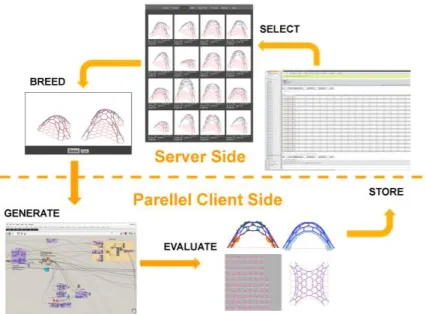
Their methodology executed in Rhino/Grasshopper consisted of 4 steps: 1) selecting a base topology grid (target structure), 2) executing a dynamic relaxation of the grid using the plugin Kangaroo to find a compression shell, 3) apply gravity loads using the Karamba plugin and analyze the structural implications, and 4) export the final images using the Ladybug plugin. A solutions space to find and display the best structures for the tree fork library was constructed through Paragen, a design aid developed by the University of Michigan. This system combines parametric form generation through Kangaroo and an analysis tool (Karamba); a non-destructive dynamic population genetic algorithm is applied to search for solutions that fit the applied criteria and the results are saved to a Structured Query Language (SQL) database. The process is designed to be cyclical and interactive such that clients can instantaneous react to the designs created through the solution exploration (Von Buelow, Peter, et al. 2018). The basic design process is shown in Figure 13.

Figure 13. The basic ParaGen cycle showing the steps used to generate a range of solutions (Von Buelow, Peter, et al. 2018, 5)

1.3.4 Designing with existing materials

The contemporary mindset for structural engineering is a design of abundance and standardization; there is an assumption that there are infinite supplies of reoccurring elements. This approach does not work for instances where structural materials are available in finite quantities or not available at all, and design mentality must change to use resources more mindfully. Additionally, environmentally and economically there is an interest to design with less embodied carbon or amount of material through structural optimization, usage of local materials, or utilization of new technologies. There have been some custom enterprises utilizing found tree forms, such as specializing in ad hoc railings made from branches, but these ventures tend to have an artisan component that is difficult to implement at a larger scale. Conventional approaches for finding solutions with finite quantities of material, methods to reuse existing material, or designs based on an available material library are slow or ineffective, requiring time-consuming trial and error to

(22)

develop viable designs, or not findings solutions at all. New computational strategies are key to tackling this problem and developing methodologies of using existing materials in design. Brütting et al. (2018) researches the reuse of structural components in design to reduce the environmental impact of building structures. Their work utilizes structural optimization formulations to design truss systems from reusable steel elements; weight minimization and embodied energy serve as objective functions subject to ultimate and serviceability constraints. The methodology utilized in their research is a two-step method in which the original structure undergoes a topology optimization followed by a geometry optimization. Specific case studies were conducted on: 1) simple roof truss systems with predefined geometry and topology and 2) geometry optimization to better match the optimal topology found for trusses in the form of a simple cantilever, a bridge (Figure 14), and a complex roof with available stock length elements. In each of these case studies, Brütting et al. (2018) compares the structural shape, size of the members, mass, embodied energy, displacement, and element capacity utilization between the structure made from reused elements versus new material. The result of the optimized shape for the bridge truss is shown in Figure 15 and the compared values are in Figure 16. This research concludes that even though structures made from reused elements have a higher mass and lower element capacity utilization, they embody significantly less energy and carbon with respect to structures made of new elements (Brütting et al. 2018, 19). The two-step methodology is sufficient to locate local optima, but a more efficient solution explored in the present tree fork optimization would simultaneously optimize element assignment, topology, and geometry.

Figure 14. Bridge truss system – ground structure (Brütting et al. 2018, 18)

(23)

Figure 16. Bridge truss – assignment optimization (Brütting et al. 2018, 19)

Bukauskas et al. (2018) explores naturally-occurring small-diameter round timbers as a viable existing structural material to be utilized with minimal processing. The group has developed an approach that makes it easier for engineers and architects to design using these low embodied-energy, inventory-constrained materials. Bakauskas et al. has proposed the concept of an

“assignment” of inventory elements to structural elements, which is a set of instructions necessary

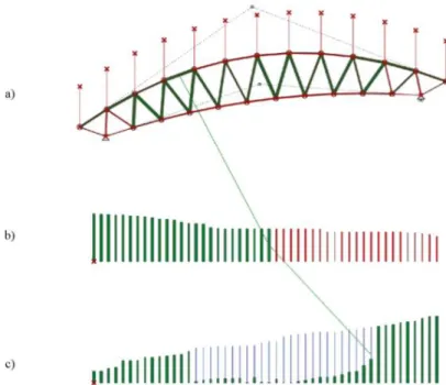
to assemble a structure from the given set of inventory elements. Additionally, rather than minimizing the structural problem for mass or structural stiffness, an offcut-ratio, the ratio of offcut waste mass to the mass of inventory material consumed, is applied. The off-cut ratio better for this instance, because it is a helpful benchmarking tool when comparing the relative performance of assignments for different designs. An example of this methodology can be seen in Figure 17 of how a designer can use this approach to parametrically design a roof truck with a constrained inventory (Bakauskas et al. 2018, 8).

(24)

Figure 17. Iterative form-finding process for inventory constrained design: a) parametrically defined structure with loads and support conditions b) structure elements pre-sorted in descending order by length, c) inventory elements pre-sorted in ascending order by length

(Bakauskas et al. 2018, 8)

Previous work regarding using existing materials has focused on finding specialized solutions for truss structures reusing steel elements as well as developing a specific metric for usage of small-diameter round timbers. The research presented in this thesis aims to understand tree forks as an existing material and develop a comprehensive scoring metric for matching and performance of proposed structural designs. With continued research in this field, modern technology, when applied, will make designing with available materials more accessible and available reality for the future.

1.4 Research objective

This project will focus on two goals: 1) exploring the extent and limitations of the material library on the structural design by conducting a thorough sampling of tree fork nodes of various tree species found at the site location, and 2) creating a model that allows the user to understand the relationship between varying the geometry, the number of tree forks in the material library, the structural percentage match of the tree fork vector angles to the nodes and the percent allowable variation in the geometry of the original structure. The above plans will be carried out through physical structural tests as well as software analysis through Grasshopper in Rhino. The research question posed for the matching-based design method and structural performance of tree nodes are listed.

(25)

Matching-based design method:

1) How many samples are necessary to get the “best match” for a desired structure? Is there

a point where the matching score exhibits diminishing returns as number of samples in the material library increases?

2) How do various tree species perform on different target geometries?

3) What is the relationship between tree species, number of samples, and target geometry? 4) What is the ratio of tree nodes available to inventory size needed that results in a good

match?

Structural performance of tree branch nodes:

1) What kind of reaction (e.g. splitting, crushing, cracks, etc.) occurs during a moment test of a tree fork branch?

2) Is there an angular cutoff in which there is a significant decrease in performance of tree forks?

3) Which tree species provides the best structural score? Which tree species is recommended for use in structural design?

(26)

2 Matching-based design methods and results

2.1 Conceptual overview of design process

2.1.1 Previous work

Previous work has been conducted by Caitlin Mueller, Felix Amtsberg, Kevin Moreno Gata, and Yijiang Huang in designing an algorithm to fit natural tree fork connections into a pre-described structure. Their research goal was to quantify the mismatch between a three-valence node on a design geometry and a tree fork and to create a computational algorithm to find the optimal

matching that minimizes the overall “mismatch error” calculated. A material library was collected

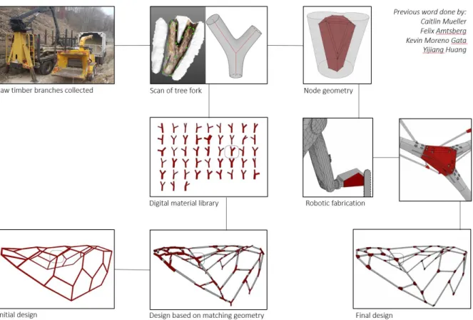
and analyzed, a computational algorithm was developed, the available tree forks were matched to a design, robotic fabrication was utilized to cut the joints to shape, and a prototype of the design was constructed (Figure 18).

(27)

Figure 18. Process of acquiring material, digitizing inventory, designing and fabricating (Amtsberg et al.)

A library of 46 tree forks of various species were collected from Somerville, Massachusetts and catalogued for use in this project. A few examples of the tree forks obtained to be analyzed are shown in Figure 19. Low-cost 3D-scanners were used to generate a rudimentary material library from which a mesh was uploaded in Rhino to be cleaned and simplified. The Rhino model contained branch diameter and angle information to be referenced later in a computational algorithm.

(28)

An algorithm was constructed through the combination of the Hungarian algorithm and Iterative Closest Point algorithm that takes the nodal center points of the tree forks in the library and matches them to the nodal points of the pre-described structure at the best vector angle fit, which will be detailed in section 2.1.2.6 Matching score (Figure 20).

Figure 20. Iterative Closest Point (ICP) and Hungarian algorithm matching tree fork material library to given structure (Huang et al.)

The matching algorithm was used to design a small, specialized prototype that could test the design-to-fabrication process. The fabrication sequence of the matched tree forks to a proposed structure are shown in Figure 21.

Figure 21. Prototype structure (Amtsberg et al.)

This previous work provided a starting point for this research project by generating a methodology that gives a quantitative value that represents the quality of match between available tree forks in a material library to a target design. Since the matching score improves as the fit of the tree fork vectors to the structure has less variance, this thesis explores various methods that change the target structure to best match the available tree forks.

2.1.2 General methodology

In order to generate a new, simulated material library of 50, 100, 200, 250, 350, 500, 750, and/or 1000 samples, basic tree morphology data is necessary: the tree species present at the site, the branch angle range for different species, the branch diameter ratio between the main branch and the two branching out forks. With the necessary data, a new material library can be randomly generated for a project. For the purposes of this thesis, material libraries consisting of branches of the same species will be analyzed for matching ability to a prescribed structure.

(29)

2.1.2.1Tree species

The original study conducted by Caitlin Mueller, Felix Amtsberg, Kevin Moreno Gata, and Yijiang Huang was based on existing trees cut down from a high school in Somerville, Massachusetts, so for consistency, a sampling was conducted based on the trees found at that location. This data was found in the Somerville TreeKeeper database, a software website used to track the economic and ecological benefits of each tree in the city, and is shown in Figure 22 (“TreeKeeper”). Navigating through the online database, on the side panel there is an option to build a report based on site; selecting the Somerville High School option gives the number of trees of each species in that location. The main tree species at the site are: maple, crabapple, ash, dogwood, oak, and various fruit trees.

Figure 22. TreeKeeper database cataloguing all trees in Somerville, MA (“TreeKeeper”) 2.1.2.2Branch angles

The necessary tree branch angles are found through botanical tree image generation data, which provides a maximum, minimum and average branching angle. This data was collected by Masaki Aono and Tosiyasu L. Kunii from the University of Tokyo to model botanical trees through geometric modeling in a computer graphics system. Visualizations of the trees generated are shown in Figure 23. Since the trees sampled are in Japan, a common genus (i.e. birch or ash or maple) and similar characteristics of the trees were cross-referenced between the data collected by Aono and Kunii (1984) and the Somerville High School tree species (19). This information is shown in Table 1; the tree name is from the paper followed by the common name/characteristics, its match to the Somerville High School tree, the total number of that species in Somerville, and the average/maximum/minimum angle data. In Grasshopper, the branching angle variable range is set between the minimum angle divided by 2 to the maximum angle divided by 2 for the right and left branch angle. A third z-angle variable is set for the right and left forks at a range of zero to 30 degrees as evidenced from literature and the original data library (Pradal et al 2008).9

(30)

Figure 23. Visualizations of tree image generation data based on collected branching angles (Aono and Kunii 1984, 15)

Table 1. Tree fork average, minimum, and maximum angles

Tree Name Common

Name/Characteristics Match to location tree type # of species at location (Total = 14k) Aver. Angle Max. Angle Min. Angle

Betula platyphylla Birch Birch 173 60 86 35

Cornus controversa Dogwood, med-size,

deciduous Dogwood 71 60 88 40

Liquidambar formosana Sweet gum, deciduous Ash 1052 64 99 25

Lithocarpus edulis Stone-oak Oak 730 54 86 32

Myrica rubra small-med-size, fruit tree Crabapple 208 60 85 30 Liriodendron tulipifera Poplar, large, deciduous Maple 7 56 83 25

2.1.2.3Tree branch diameters

Tree branch diameters were obtained through utilization of Leonardo da Vinci’s rule, which states that the sum of the cross-sectional area of all tree branches above a branching point at any height is equal to the cross-sectional area of the truck or branch immediately below the branching point (Minamino and Tateno 2014). This rule is visually displayed in a computer-simulated tree example in Figure 24.

Figure 24. (Left) Model of tree branching. (Middle) Tree skeleton with equivalent diameters

(31)

Mathematically, this means that if a tree fork with a trunk branch diameter (D) splits into an

arbitrary number (n) of secondary branches of diameters (d1, d2, …), the sum of the secondary diameters squared equals the square of the original branch’s diameter.

𝐷2 = ∑ 𝑑_𝑖2

𝑖 (1)

The Grasshopper model sampling aims to reproduce tree forks similar in size to those previously scanned and recorded within the material library with reasonable variability. The trunk branch diameter varies between 6 and 10 inches, and one of the forking branches varies between 3 and 5 inches. The random sampling selects a value within these ranges and subsequently calculates the

last forking branch diameter according to Leonardo da Vinci’s rule.

2.1.2.4Methodology for simulating random tree fork library

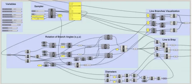
Since there is a generous amount of variability even within each tree species depending on various environmental and location specific factors, a random sampling of the tree image data provides a satisfactory database for the simulated tree forks. A random uniform sampling is completed in Grasshopper for Rhino through the Sampling component found in the Design Space Exploration plugin. The five variables inputted into the Sampler are: 1) the right branch angle, 2) the left branch angle, 3) z-axis rotation angle, 4) diameter of the trunk branch, and 5) diameter of one of the forks. A sampling is conducted for the three most common species in the Somerville High School location: ash, oak, and crabapple for 50, 100, 200, 250, 350, 500, 750, and/or 1000 samples. This information is then inputted into the Grasshopper code that takes the values and creates tree fork representations that can be inputted into the matching algorithm. This process is shown in Figure 25. The “Rotation of Branch Angles” and “Line Branch Visualization” section takes the angle values and creates line representations (Figure 26), and the “Diameters” and “Line to Brep” sections create pipe representations to be displayed in the Rhino model (Figure 27).

(32)

Figure 26. Line representations of tree forks Figure 27. Brep pipe representations of tree forks

The newly generated samples are then input into the Grasshopper code that vectorizes and matches the nodes to the structure.

2.1.2.5Target structures

The prototype structures are designed within Grasshopper to allow for geometric variation through either control curves or points, changing the variables that manipulate these components alters the geometry of the structure. The computational matching algorithm automatically updates the tree forks matched to each node for the best fit as the geometry changes, which allows for an optimization algorithm to use the control curves or points as variables and the matching score as a minimization objective. This geometric variation aims to answer the research question of whether or not there is a best fit structure that fits the tree forks available in a material library.

The structures simulated in Grasshopper within this thesis aim to limit the number of variables used to manipulate the geometry of the structure while maintaining a generous control space for the structure to shape to multiple forms. An unsuccessful iteration that designated each x, y, and z-value of each node a variable resulted in erratic geometries and nonconvergence when optimized. Additionally, when designing potential structures as options for utilizing the tree forks simulated in the sampling and subjected to the computational matching algorithm as structural nodes, it is important to ensure that the prototype structure’s nodes have three beam elements meeting at each singular joint. Any nodal configurations with more or less than three vectors meeting at joint causes an error within the computational algorithm resulting in no matching.

2.1.2.6Matching score

A computational model was constructed through the combination of the Hungarian algorithm and Iterative Closest Point algorithm to develop 1) a metric calculating the mismatch between the tree fork vectors to matched nodal vectors, known as the matching score and 2) a method of matching the tree forks in the available material library to the nodal points of a proposed structure that minimizes the overall mismatch score. The mismatch metric is defined based on the Iterative Closest Point (ICP) method and the Hungarian algorithm is used to find the minimal distance matching. As mentioned in 2.1.1 Previous work, this computational algorithm was implemented in Grasshopper by Yijiang Huang.

(33)

The matching problem formulation is fundamentally a map that uses the notion of distance to measure the gap between the vectors of the structural nodes to the vectors in the tree forks, and it can be formulated as:

min

𝑐∈𝑃𝑒𝑟𝑚([𝑚])∑ 𝑑(𝑁𝑖, 𝑀𝑐(𝑖)) 𝑛

𝑖=1

(2) where d is the mismatch metric needed to be designed, Ni represents the n three-valance structural

target nodes where i ϵ {1, …, n}, and Mc(i) represents the n three-valance tree fork nodes where i ϵ

{1, …, n} and c(i) is the integer index of the point in M that corresponds most closely with the

i-th point in N.

The ICP is implemented first and computes the mismatch metric, d, between a design node N and tree fork M by finding the optimal rotation, translation, and distance to vectors of the structure’s node and then computing the sum of squared matched end point distances. Three vectors generate a central line skeleton that represents each target structure node and each tree fork in the material library. The set of three vectors use the four end points of the skeleton line segments: 𝑁_𝑖 = {𝑢₀𝑁𝑖_{, 𝑢} 1 𝑁𝑖_{, 𝑢} 2 𝑁𝑖_{, 𝑢} 3 𝑁𝑖_{} and 𝑀} 𝑖 = {𝑣0 𝑀𝑖_{, 𝑣} 1 𝑀𝑖_{, 𝑣} 2 𝑀𝑖_{, 𝑣} 3 𝑀𝑖_{}, where 𝑢} 0 𝑁𝑖_and_𝑣 0

𝑀𝑖_{are the central points that}

have a valence of three. A joint optimization of rotation, translation, and skeleton line correspondence produces a distance, so the mismatch measure problem can be formulated as matching the two vectors sets:

𝑑(𝑁, 𝑀) ≔ min 𝑅,𝑡,𝑐∑‖𝑅 ∙ 𝑢𝑖 𝑁𝑖 + 𝑡 − 𝑣_𝑐(𝑖)𝑀 ‖ 2 2 3 𝑖=0 𝑠. 𝑡. 𝑅𝑡= 𝑅−1, 𝑅 ∈ 𝑹3 𝑡 ∈ 𝑹3 (3)

The Iterative Closest Point algorithm alternates between solving for Rotation, R, translation, t, and the correspondence, c, separately and then finds the closest rotated and translated tree fork. Theorem: Let 𝑋′ _{= {𝑥} 𝑖− 𝜇𝑥|𝑖 ∈ [𝑛]|} = {𝑥𝑖′} and 𝑃′= {𝑝𝑖− 𝜇𝑝|𝑖 ∈ [𝑛]|} = {𝑝𝑖′}𝑃′ where 𝜇𝑥 = 1 𝑛∑ 𝑥𝑖 𝑛 𝑖=1 and 𝜇𝑝 = 1 𝑛∑ 𝑝𝑖 𝑛

𝑖=1 denotes the center of masses. Let W = ∑𝑛𝑖=1𝑝𝑖′∙ 𝑥𝑖′𝑇, and its

Singular Value Decomposition, SVD, is 𝑊 = 𝑈 [

𝜎1 0 0

0 𝜎₂ 0

0 0 𝜎3

] 𝑉𝑇, where 𝑈, 𝑉 ∈ ℝ3𝑥3 are

unitary and 𝜎1 ≥ 𝜎2 ≥ 𝜎3 are the singular values of W. Then, if the rank(W) = 3, the optimal

solution of 𝐸(𝑅, 𝑡) = 1

𝑛∑ ‖𝑅 ∙ 𝑥𝑖+ 𝑡 − 𝑝𝑖‖

2 𝑛

𝑖=1 is unique and given by:

𝑅∗ = 𝑈 ∙ 𝑉𝑇 (4)

𝑡∗ = 𝜇_𝑝− 𝑅∗∙ 𝜇_𝑥 (5)

The minimal value of the error function, known as the matching score, is 𝐸(𝑅∗, 𝑡∗) =

(34)

The Hungarian algorithm, a combinatorial optimization algorithm, is processed on each of the node vector matches to minimize the distance difference between the tree fork vector and the structural node vectors and gives a matching score value. It takes the distance 𝑑, which measures

the mismatch, a mismatch distance matrix 𝐷 ∈ ℝ 𝑛×𝑚 can be constructed by having 𝐷𝑖𝑗 = 𝑑(𝑁𝑖 , 𝑀𝑗). Then, the Hungarian algorithm takes this distance matrix 𝐷 as an input and outputs the

optimal match, c (“The Hungarian Algorithm”). An open source C# implementation of the Hungarian algorithm is used in the Rhino/Grasshopper environment.

The mismatch metric generated in Equation (3 can be solved through the following steps:

1. Given an initial R and t, the correspondence, c, is calculated by calculating the Euclidean distance through the Hungarian Algorithm.

2. Use c to solve R* and t* using Equations (4 and (5

3. If the new mean error, matching score, 1

4∑ ‖𝑅 ∙ 𝑢𝑖 𝑁𝑖_{+ 𝑡 − 𝑣} 𝑐(𝑖)𝑀 ‖ 2 3 𝑖=0 does not

exhibit any change within a specified tolerance since the last iteration, then go to step 1 and repeat, otherwise exit.

The matching score is the tabulated as the mean error for the whole structure of all the matched tree forks to the target structure nodes; the Hungarian algorithm calculates the Euclidean distances between the tree forks and target nodes resulting in the R, t, and c values and the iterative closest point theorem outputs the mean error, matching score, described above as 𝐸(𝑅∗_{, 𝑡}∗_{) =}

∑𝑛 (‖𝑥_𝑖′‖2₊

𝑖=1 ‖𝑝𝑖′‖2) − 2(𝜎1− 𝜎2− 𝜎3) tabulated from inputting Equations (4 and (5 into

Equation (3.

The larger the matching score value, the worse the matching result, so a minimal matching score

is desired for a “good” matching structure.

2.1.2.7Optimization

In this research thesis, structural optimization formulations are utilized to design target structures from available tree forks in a material library. Minimization of the matching score is the objective function subject to target structure geometry design variables.

The optimization is conducted in a built-in component in Grasshopper, Galapagos. This optimizer tool is able to optimize a shape so that it best achieves a user defined goal. For the Galapagos

component to work, it needs a series of variables or “genes” to sample, and a defined objective or “fitness value.” In the geometries tested in the following case studies, the variables adjusting the 2 control curves, 5 control points, and 1 control curve are the input “genes,” and for all the cases, the matching score is the “fitness value.” Galapagos does not try every single possible combination

of the options to find an optimum solution; instead, it aims to “learn” from each successive round

of experiments or “generations” to progressively get to the best answer.

Within Galapagos, the Simulated Annealing solver was utilized to minimize the matching score (the lower the score, the better the match). Simulated annealing is a heuristic optimization method, which uses random numbers and statistical methods to improve a design until a satisfactory result is reached. This method, though effective for optimizations in a large sample space, may still

(35)

provide a local minimum depending on the starting point of the problem. For consistency in the sampling results, the target structure geometry was reset to the original structure before a new optimization was conducted.

The colors of the tree branches matched to the target structure qualitatively and relatively demonstrate the better and worse matches for the tree fork to structural node. Colors range from green to yellow to orange to pink representing best to worse matches; an example of the color matching is seen in Figure 28 for a 4x7 hexagonal grid target structure with oak tree forks matched. It would be optimal to have a matching score equal to zero and all representative tree forks to be colored green.

Figure 28. Oak. 4x7: Hexagonal, 1 Control Curve. 100 samples.

2.2 Simulated inventories and case studies

There are 46 samples in the original digital material library; the new sampling method coded within Grasshopper generates any number of tree forks for the computational matching algorithm to correspond to the nodes to any designed template structure. This research comprises of iterated samplings of the material library on three distinct protype structures to investigate three questions:

1) how many samples are necessary to get the “best match” for a desired structure, at what point

are there diminishing returns? 2) are some geometries better target structures than others? 3) what tree species have the best fit for the structures tested?

The geometries are matched with three commonly found tree species found from the original material library location in Somerville, Massachusetts: ash, oak, and a wide-ranging fruit species. These tree species were correlated to trees sampled in Japan through a common genus that has the same characteristics to obtain the angular tree morphology data collected in the study done by Aono and Kunii explained in section 2.1.2.2 Branch angles. The angles for the ash, oak, and fruit tree are shown in Table 2.

(36)

Table 2. Ash, oak, and fruit tree branch angles

Ash Oak Fruit

Angles: Average: 64 Angles: Average: 54 Angles: Average: 60

Maximum: 99 Maximum: 86 Maximum: 85

Minimum: 25 Minimum: 32 Minimum: 30

2.2.1 Pavilion geometry with 2 control curves (4 variables)

The initial structure used for the sampling analysis is the original pavilion from previous work designed for a high school in Somerville, Massachusetts where the tree forks were collected. The original structure was modeled by Mueller, Amtsberg, and Gata in Rhino (Figure 29a), and its shape can be manipulated with two control curves generated in the Grasshopper environment (Figure 29b). The two lines of curvature have four variables that control the strength and amount of curvature the structure follows (Figure 29c).

a. Initial geometry b. 2 Nurbs curves defining geometry

c. 4 variables/control points change curvature d. optimized shape according to new curvature

Figure 29. Pavilion geometry with 2 control curves

The geometry of the target structure changes based on the two control curves such that the nodes on the structure shift according to the curvature changes (Figure 29d). The Galapagos optimizer plugin is utilized to vary the four variables controlling the curvature shape of the structure to

(37)

minimize the matching score by automatically placing the best fit tree forks from the generated material library onto the target structure.

An iteration of the original pavilion geometry was tested by changing the variables from the broad control curves to the x, y, and z-coordinates of each node of the target structure. The reasoning for this approach speculated that if the x, y, and z coordinates of the target structure are able to be shifted within a range, then there will be a structure that has a matching score equal to zero where every tree fork is a theoretical perfect fit to the target structure. This trial was unsuccessful for two reasons: 1) the optimization failed to converge on a single solution because there were too many variables, and 2) if a solution was found, it was incongruous and therefore, unlikely to be a viable architectural shape. A potential geometry using this control point system is shown in Figure 30.

Figure 30. Potential geometry given x, y, z-coordinate variables for each node 2.2.2 Hexagonal geometry with 5 Control Points (5 variables)

To understand the sampling effects of the tree fork matching on a more conventional geometry, a hexagonal grid of varying x-direction and y-direction densities was generated and projected on a surface with 5, z-direction control points. Hexagonal grids are distinctive in that every node has three beam elements meeting a singular connection point, so a hexagonal surface is a model target geometry for tree fork matching. The process of generating the hexagonal grid and projecting it on a square surface constructed from 9 points is shown in

(38)

a. 9 surface construction points

b. generated surface from 9 points

c. 5 edge control points with variable z-coordinates

d. projected hexagonal grid on surface e. hexagonal surface target surface

f. columns for hexagonal geometry g. matched tree forks for hexagonal geometry Figure 31. Hexagonal surface geometry generation process

The results of the sampling experiments are discussed in section 2.3.2 Hexagonal geometry with 5 control points (5 variables) results.

2.2.3 Hexagonal geometry with 1 Control Curve (3 variables)

The hexagonal initial geometry was iterated to create a more rigid geometry with fewer variables to create more consistent final geometries. The hexagonal grid now has fixed connections along the edge points in the x-direction, and the curvature of the structure is manipulated with 3 variables

composing one control curve. The base surface the hexagonal grid is projected on is 20’x20’

square. The x-direction hexagonal grid density controls the number of support points fixed to the ground, and the y-direction hexagonal grid density represents the number of hexagons across the target structure. The number of hexagons in the x and y-direction are varied to observe if varying the initial grid structure while all other variables remain constant would produce varying matching score results answering the question, are some geometries better target structures than others? The geometry controlling the curvature of the structure is a non-uniform rational b-spline, NURBS, curve, which is a mathematical formulation that has a high level of flexibility and precision restrained by a set of control points. The singular NURBS curve controlling the hexagonal geometry has three variables: 1) the height of the lofted curve, 2) the degree of curvature, and 3) an angular x-rotation of the curve. This NURBS curve dictates the final surface through three

(39)

additional NURBS curves formed from the endpoints and midpoints of the NURBS curve and the two x-direction edges fixed at the ground (Figure 32). An assortment of the geometric variations resulting from altering the variables that control the NURBS curve are shown in Figure 33 and Figure 34.

(40)

Height of lofted curve = 1.5 Degree of curvature 0.5 1.0 1.5 2.0 Curve angular x-rotation -30 -15 0 15 30

Figure 34. Curve angular x-rotation vs. degree of curvature geometry representation with constant height of lofted curve

Curve angular x-rotation = 0 Degree of curvature 0.5 1.0 1.5 2.0 Height of lofted curve 1.5 2.0 2.5

Figure 33. Height of lofted curve vs. degree of curvature geometry representation with constant curve angular x-rotation

(41)

The hexagonal geometry with one control curve is optimum for a scenario in which a particular final geometry configuration is desired; there is ample geometric variation with the variable constraints which allows for analogous final geometries. Extensive sampling tests were conducted for material library sizes of 50, 100, 200, 350, and 500 tree forks and for all combinations of varying the number of hexagons in the x and y-direction ranging from 3 to 7, inclusive. This resulted in a total of 15 experiments per geometry, 5 per species for each of the material library sizes, and 25 individual geometries to test. The results of these experiments are discussed in section 2.3.3 Hexagonal geometry with 1 control curve (3 variables) results and the data is in collated Appendix B.

2.3 Results

2.3.1 Pavilion geometry with 2 control curves (4 variables) results

The matching score results for the sampling of the original pavilion geometry for 50, 100, 250, 500, 750, and 1000 samples are shown in Table 3 and graphed in Figure 35. The data shows that the ash species has a significantly better matching score for each number of samples. This can be attributed to the wider maximum angle of ash; oak and fruit have no variation in their maximum angle value and slight variation in their minimum angle value resulting in expected overlapping results. The wider angle in ash producing better matching scores may also be specific to this original pavilion structure provided. A different original structure with narrower angles may result in a different outcome, which suggests results can be highly dependent on the starting structure; further testing is suggested to validate this claim.

The point of diminishing returns at which increasing the number of samples does not improve the matching score occurs at 500 samples, which is about ten times the number of nodes on the structure. Geometries generated with greater than 100 samples are considered good matches, since the most significant improvement in matching score (15-26% decrease) occurs between 50 and 100 samples. Matching score improvements between 100-250 samples and 250-500 samples are significant with an 8-18% and 12-18% decrease, respectfully, so if the number of tree forks are available for these material library sizes, it would be preferred in a design scenario. Additionally, there is an exponential time tradeoff as the number of samples is increased; the more samples, the more time required to conduct the sampling and matching: 50, 100, and 250 samples take a couple minutes, 500 samples take about 10 minutes, 750 samples take about 20 minutes, and 1000 samples take about 30 minutes.

(42)

Table 3. Optimized pavilion geometry sampling matching score results

Ash Oak Fruit

Angles: Aver: 64 Angles: Aver: 54 Angles: Aver: 60

Max: 99 Max: 86 Max: 85

Min: 25 Min: 32 Min: 30

# of

samples Matching Score

50 25,331 47,251 44,405 100 18,646 35,312 37,993 250 17,105 31,834 31,338 500 13,943 27,228 27,559 750 13,347 28,341 26,735 1000 13,320 26,519 26,245

Figure 35. Original pavilion geometry Matching Score vs. # of Samples

0 5000 10000 15000 20000 25000 30000 35000 40000 45000 50000 0 250 500 750 1000 Ma tchi ng Scor e # of Samples

(43)

2.3.2 Hexagonal geometry with 5 control points (5 variables) results

This hexagonal geometry was examined briefly in conjunction with the sampled tree fork libraries, but due to the structural implications of the design further testing was ceased. The pinned columns at the corner points of the surface would experience a sizeable horizonal thrust force that would be difficult to resolve with a matched tree fork member. A more comprehensive structural solution would be necessary to address this design challenge.

The advantage of this hexagonal geometry with 5 control points is that for each sampling scenario varying the number of samples and the number of hexagons in the x and y-direction, there was a considerable amount of geometric variation. This geometry manipulation with a moderate number of variables is a useful option for brainstorming potential final geometries and scenarios where no specific configuration is desired for the structure.

The conducted sampling results are collated in Appendix A for a 9’x21’ surface with a projected hexagonal grid with a fixed x-direction hexagonal density of one and a varying y-direction hexagonal density ranging from two to nine. For each of the hexagonal grid geometries, material library sizes of 50, 100, 250, 350, 500, and 750 tree forks were generated and matched to the target geometry to be optimized for matching score performance. Only the ash tree species was implemented in this brief case study.

The matching score incurred an exponential decrease when the number of samples increased, as expected. An acceptable matching score was available at just 50 samples in the material library justified by the low ratio of number of structural nodes to number of tree forks as well as the high degree of variation in the geometry promoting more accurate fits to the available tree forks. Each successive iteration of the hexagonal geometry with increased samples resulted in a wide range of geometries as seen in Figure 37 obtainable due to the appreciable z-direction range of the 5 control points.