Publisher’s version / Version de l'éditeur:
2017 IEEE 30th Canadian Conference on Electrical and Computer Engineering
(CCECE), 2017-06-15
READ THESE TERMS AND CONDITIONS CAREFULLY BEFORE USING THIS WEBSITE. https://nrc-publications.canada.ca/eng/copyright
Vous avez des questions? Nous pouvons vous aider. Pour communiquer directement avec un auteur, consultez la première page de la revue dans laquelle son article a été publié afin de trouver ses coordonnées. Si vous n’arrivez pas à les repérer, communiquez avec nous à PublicationsArchive-ArchivesPublications@nrc-cnrc.gc.ca.
Questions? Contact the NRC Publications Archive team at
PublicationsArchive-ArchivesPublications@nrc-cnrc.gc.ca. If you wish to email the authors directly, please see the first page of the publication for their contact information.
NRC Publications Archive
Archives des publications du CNRC
This publication could be one of several versions: author’s original, accepted manuscript or the publisher’s version. / La version de cette publication peut être l’une des suivantes : la version prépublication de l’auteur, la version acceptée du manuscrit ou la version de l’éditeur.
For the publisher’s version, please access the DOI link below./ Pour consulter la version de l’éditeur, utilisez le lien DOI ci-dessous.
https://doi.org/10.1109/CCECE.2017.7946620
Access and use of this website and the material on it are subject to the Terms and Conditions set forth at
Regression based algorithms for predicting age of an Arabidopsis plant
Panjvani, Karim; Dinh, Anh; Wahid, Khan; Bhowmik, Pankaj
https://publications-cnrc.canada.ca/fra/droits
L’accès à ce site Web et l’utilisation de son contenu sont assujettis aux conditions présentées dans le site LISEZ CES CONDITIONS ATTENTIVEMENT AVANT D’UTILISER CE SITE WEB.
NRC Publications Record / Notice d'Archives des publications de CNRC:
https://nrc-publications.canada.ca/eng/view/object/?id=d44b69a3-cfe5-4f67-8fe2-abedd9181ff5 https://publications-cnrc.canada.ca/fra/voir/objet/?id=d44b69a3-cfe5-4f67-8fe2-abedd9181ff5Regression Based Algorithms for Predicting Age of
an Arabidopsis Plant
Karim Panjvani, Anh Dinh, Khan Wahid
Department of Electrical and Computer Engineering University of Saskatchewan
Saskatoon, Canada
karim.panjvani@usask.ca
Pankaj Bhowmik
National Research Council Canada Saskatoon, Saskatchewan
Canada
pankaj.bhowmik@nrc-cnrc.gc.ca
Abstract— This paper presents the analysis of various
regression based machine learning algorithms for image-based plant phenotyping application and proposes a technique for plant phenotyping. Capability to predict age/development stage of a plant is one of the important factors for plant phenotyping and for analysis of in-situ crops. With the developed technique, these algorithms can predict age of an Arabidopsis plant based on the given images and mutant types. Publicly available dataset containing 165 images at different development stages and with various mutant types was used for this experiment. Results show that with this technique and different regression algorithms, it can achieve 92% prediction accuracy. Comparatively, linear regression algorithms show greater prediction accuracy than non-linear algorithms. This method of age prediction can help plant scientists and breeders for better analysis of crops.
Keywords—Age prediction, plant phenotyping, machine learning, pattern recognition in plant imaging
I. INTRODUCTION
As per the Food and Agriculture Organization (FAO) of the United Nations (UN), large scale experiments in plant phenotyping are a key factor in meeting agricultural needs of the future, one of which is feeding 11 billion people by 2050. “Plant phenotyping is the comprehensive assessment of complex plant traits such as growth, development, tolerance, resistance, architecture, physiology, ecology, yield, and the basic measurement of individual quantitative parameters that form the basis for the more complex traits” [1]. Imaging in plant phenotyping aims to automate the process of evaluating growth and phenotypic properties [2]. For example, study of a leaf structure of a plant gives an idea of its maturing time, i.e., readiness for harvesting. Moreover, having knowledge of similarities in plants that went under different treatment can lead to development of new methods for developing new crop traits. Hence, the problem of identifying age of a plant based on the provided image is one of the key factors to know for breeders and plant researchers. There have been many studies for phenotyping a plant with visual components by manual observations with the help of experts, but this task is laborious and takes a tremendous amount of time. Hence, there is a need for image-based methods to automate these efforts [3]. Plant image analysis software researches, such as “Image Harvest” are playing key role for image based plant analysis [4].
Predicting an age of a plant is still a difficult task. However, with the use of imaging technology and machine learning
algorithms, it can be easy and accurate up to certain level. There are some publicly available databases for plant-phenotyping that can be used to make a decent decision [3,5,6]. As compared to DNA or other medical imaging datasets currently available, plant phenotyping is still lacking of standard datasets for use in machine learning algorithms. One of the available datasets that for Arabidopsis and tobacco plants is available in [7]. This dataset includes raw RGB (Red, Green and Blue) images and mutant types, treatment types and the age after germination combined in a single meta-data file [3]. There are several algorithms available for prediction/regression problems in machine learning, one of them is “gradient descent” [8]. Regarding software, python is an open-source programming language driven by like-minded people who believe in free and widely accessible platform. Scikit-learn is one of the popular libraries for machine learning using python. It provides most of the popular algorithms for machine learning already implemented [9,10].
An image is a matrix of values corresponding to each pixel of that image. Generally, they are 3-Dimensional matrix with third dimension containing Red, Green, and Blue planes. As images contain many pixels, there is a need to reduce dimensionality of an image. There are various dimensionality reduction techniques available in within Scikit-learn library [10]. Regression is concerned with modeling the relationship between variables that is iteratively refined using a measure of error in the predictions made by the model. Some of the most popular regression algorithms are Ordinary Least Square Regression (OLSR), Linear Regression, Ridge Regression, Lasso Regression, and Support Vector Regression. The cost function is optimized using the number of iterations to find optimal values of the coefficients. These coefficients estimate the output value from given feature values. The goal here is to find the minimal value of coefficients in an equation to estimate output value from a given input feature values.
II. METHODOLOGY
The dataset contains raw images with their corresponding genotype/mutant type and their respective age after germination. Machine learning algorithms work great when it has comparatively lower number of features. Hence, data is converted from RGB image to features and reduced to certain numbers, which involves 1) image filtering, 2) background removal and 3) feature selection/dimensionality reduction. Minimum number of features is obtained and dataset is split into
train and test portions. This partitioned data is then used to train an algorithm and to determine the accuracy of an algorithm.
Mean_absolute_error and mean_squared_error are used as
evaluation metrics.
First, dataset (images) is imported into python environment to read the images and convert them to matrix of values. As images are of non-uniform sizes, they need to be resized. There are two approaches tried out, one is to resize them with built-in function and another is to fill the value zero (0) around image or zero padding. Fig. 1 shows a flow chart of the technique used to refine data before feeding it to the learning algorithm. If resize with internal functions is enabled, then it is resized with internal function. If not, further processing is carried out. Next step is to convert the RGB image into gray scale image.
After conversion to grayscale image, morphological opening is performed to remove some small objects from the foreground. Simple Otsu’s method for background removal is used to remove background components. Scikit-image library of python implements it in a filter module. Now, with Otsu’s threshold black & white (binary) image can be obtained, which contains binary values, where zero is black (dark) pixel and one is white (bright) pixel. If the resize with internal function is not enabled, binary image is filled with zeros (0’s) in its all four boundaries, to make it of standard size 350x350, same procedure is repeated for all 165 images. Another important step is to flatten 2D array, so that it can be appended to global array of features. This is called feature set.
Second, the feature set (n_samples x n_features) has 350 x 350 = 122,500 + 1(genotype) features, which is huge for any learning algorithm to get optimal results. There are algorithms/techniques available for dimensionality reduction, such as, Principal Component Analysis (PCA), Independent Component Analysis (ICA), and some other feature selection algorithms. PCA is one of the oldest and most popular algorithms to reduce dimensionality of a given feature set [11]. It removes the redundant components from a given input array. After dimensionality reduction, the feature set can be used with any learning algorithm.
Third, ground truth and genotype/mutant type are extracted from the meta-data file. One of the important features of this dataset is genotype of a given image. Pandas library in python provides number of functions to read from the .csv file, convert it into matrix and manipulate the data. Also, it provides functions to manipulate categorical information and convert them into numeric labels/data.
Fourth, split dataset into train and test portion, so as training and testing parts can be used to test the accuracy of an algorithm. This split data was used in next step for training and testing purpose. Here, 60% data is used for training and 40% is used for testing an algorithm to be fair with issues like over fitting.
Fifth, different regression algorithms are used for machine to learn from the data and predict age. Some of the popular regression algorithms are briefed below.
A. Linear Regression
Linear Regression is one of the most popular algorithms for solving regression problems [8]. In statistics, linear regression is a technique to find relationship between y (ground truth) and given x (feature set). In this case, it is known as multiple linear regression due to the fact that there are more than one features for each ground truth [12]. Equation for the linear regression with multiple variables is given as:
0 1 1 2 2
( ) ... n n
h xθ =
θ
+θ
x +θ
x + +θ
x (1)where, hɵ(x) is the estimated value based on given input features
and θ0…n is coefficients or weightage of each feature/input value
[3]. θ is found with what is known as cost function J( )
θ
and given as: ( ) ( ) 2 1 1 ( ) [ ( ) ] 2 m i i i J h x y m θ θ = =
− (2) where, mean squared error of estimated value and actual value is summed and divided by twice the number of samples [7].B. Rigde Regression
Ridge regression is another popular linear algorithm used for regression problems in machine learning [12]. Ridge regression solves coefficients θ using normal equation analytically in
matrix form [8]. The equation for solving for θ becomes as
shown below: 1 ( T ) T X X X y θ − = (2) where, (XT X)-1 is inverse of matrix XT X. Here, there is no need to choose alpha for optimizing θ. But, the problem here is what
if the inverse of XT X is not possible or it is singular or degenerate [3].
C. Lasso Regression
Lasso is an abbreviation for Least Absolute Shrinkage and Selection Operator (LASSO). It was first introduced in 1996 by Robert Tibshirani [13]. Mathematically, objective function to minimize is:
Fig. 1. Reading bunch of images and cleaning and creating an array of feature set RGB images Import all Resize function > Resize? RGB 2 gray No Yes Yes No “Otsu method” “Otsu threshold” Background removal Resize? Zero-padding Return 2-D Matrix No Yes
2 2 1
1
||
||
||
||
2
w samplesmin
Xw
y
w
n
α
−
+
(3) The Lasso estimate thus solves the minimization of the least-squares penalty withα
||w||1 added,α
is a constant and ||w||1 is the l1−norm of the parameter vector [14].D. Bayesian Ridge Regression
Byes Ridge Regression is mostly similar to classical ridge regression explained above and is derived from Bayes Regression [14].
E. Support Vector Regression
The method of Support Vector Machine (SVM) can be expanded to solve regression problems. This is known as Support Vector Regression (SVR). There are various kernels available, such as, ‘linear’, ‘sigmoid’, ‘rbf’,’poly’. ‘rbf’ kernel was used for this experiment.
These algorithms are used to find the one that can work efficiently for the given data. These algorithms are initialized and trained with training data then tested with the test data to find the mean_absolute_error and mean_squared_error.
III. EXPERIMENTAL PROCEDURE AND DATA PROCESSING The dataset is publicly available and can be downloaded from [7]. In this experiment, data that are used are only of Arabidopsis “Ara2013-Rpi”. Image acquisition was done with robotic arm and only top view of the images was released. Additional details regarding imaging setup can be found in [5]. Raw image data are annotated by experts with computer vision tasks in mind. Authors of the dataset suggest that two of the data for age regression problem, 165 images from Ara2013 (Canon) and Ara2013 (RPi) each, which are same images taken with different cameras. Also, authors of the dataset also recommend that the mean_absolute_error and the mean_squared_error to
be criterion for age regression problem. Ground truths are available in a separate .csv file, containing image name, mutant type, treatment type and age after germination, respectively [3]. Snippet of images and data used is given in Fig. 2.
The only issue with this dataset is that the RGB images are not of uniform size, i.e., the dimension of each image is different. Sometimes, having internal resize function produces some issues in detection and some of the images are not clear.
IV. RESULTS AND EVALUATION
Arabidopsis plant age prediction task is performed and
mean_absolute_error and mean_squared_error are recorded as
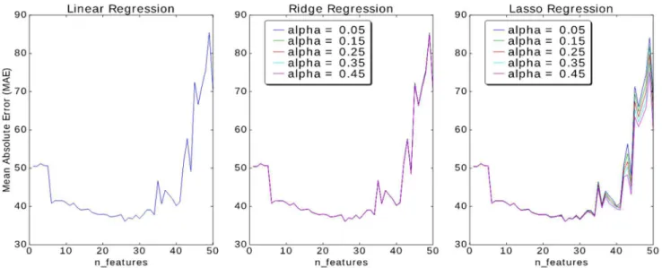
a function of number of features for 3 algorithms: Linear Regression, Ridge Regression, and Lasso Regression. Fig. 3(a) shows the performance in terms of Mean Absolute Error in hours with respect to the number of features selected after dimensionality reduction. It reveals that for 60:40 train-test-split, data with around 20-25 features gives optimal result, i.e., MAE>40 hours.
Fig. 2. Raw images and mutant type information
Fig. 3. Mean Absolute Error (MAE) as a function of Number of Features in (a) Linear Regression, (b) Ridge Regression, and (c) Lasso Regression with changing alpha
Ridge Regression algorithm was also tried with different values of alpha and number of features. It shows that the value of alpha does not impact that much compared to the number of features. Fig. 3(b) shows Mean Absolute Error (MAE) as a function of alpha and the number of features in Ridge Regression. As shown, alpha does not impact as much as the number of features does. Lasso Regression performs almost similar to the other two algorithms. But, here alpha does make a slight difference. Fig. 3(c) shows the graph of performance of the algorithm with respect to changing alpha and number of features. Out of the three, it seems that Ridge Regression works well with this dataset. All five algorithms, i.e., Linear Regression, Ridge Regression, Lasso Regression, Bayesian Ridge Regression and Support Vector Regression (SVR) are tried with default initial values set by python, and the results are compared for 24 numbers of features. Mean Absolute Percentage Error (MAPE) is not available in the python metrics library and implemented using Eq. (5).Table I shows the performance of 5 different algorithms in terms of Mean Absolute
Error (MAE) and Mean Squared Error (MSE). Linear
regression accuracy is approximately 93%.
1 _ _ 100 _ n i i i i y actual y pred MAPE n = y actual − =
(4)Fig. 4 shows the correlation between actual age of the plants and the age detected with various regression algorithms explained in this paper, for 50 test examples. Estimated ages are more accurate with linear regression algorithms than with non-linear.
V. CONCLUSION
A new simple and computationally efficient technique have been proposed in this paper. Various regression based machine
learning algorithms have been applied and analyzed using the proposed technique. Results show that linear regression algorithms work well with “Plant Phenotyping Dataset”, which was made publically available by Minervini, et al. [7].
Mean_absolute_error recorded was 36 hours.
Mean_absolute_percentage_error is 7-8% which means it can
be 92-93% accurate. Deep learning algorithms may be more accurate than linear algorithms, but at the same time, it will need more computational power. In the future, datasets on variety of plants will be used to test the performance of the proposed technique.
ACKNOWLEDGMENT
The authors would like to acknowledge the support from the Global Institute for Food Security, Canada, and Agriculture Development Fund, Saskatchewan, Canada.
REFERENCES
[1] Lemnatec, “Plant Phenotyping, Plant Phenotype,” Available: http://www.lemnatec.com/plant-phenotyping/ , accessed January 17, 2017.
[2] N. Fahlgren, M. A. Gehan, and I. Baxter, “Lights, camera, action: Highthroughput plant phenotyping is ready for a close-up,” Current Opinion in Plant Biology, vol. 24, 2015, pp. 93–99.
[3] M. Minervini, A. Fischbach, H. Scharr, and S. A. Tsaftaris, “Finelygrained annotated datasets for image-based plant phenotyping,” Pattern Recognition Letters, vol. 81, 2016, pp. 80–89.
[4] A. C. Knecht, M. T. Campbell, A. Caprez, D. R. Swanson, and H. Walia, “Image harvest: An open-source platform for high-throughput plant image processing and analysis,” Journal of Experimental Botany, vol. 67, no. 11, 2016, pp. 3587–3599.
[5] S. Hanno, M. Massimo, F. Andreas, and T. S. A., “Annotated image datasets of rosette plants,” Tech. Rep., Available: http://juser.fz-juelich.de/record/154525 , accessed January 17, 2017.
[6] M. Minervini, M. M. Abdelsamea, and S. A. Tsaftaris, “Image-based plant phenotyping with incremental learning and active contours,” Ecological Informatics, vol. 23, 2014, pp. 35–48.
[7] M. Minervini, A. Fischbach, H. Scharr, and S. Tsaftaris, “Plant phenotyping datasets,” Available: http://www.plant-phenotyping.org/datasets , accessed January 17, 2017.
[8] A. Ng., “Machine learning,” Available: https://www.coursera.org/learn/machine-learning , accessed January 17, 2017.
[9] F. Pedregosa, G. Varoquaux, A. Gramfort, V. Michel, B. Thirion, O. Grisel, M. Blondel, P. Prettenhofer, R. Weiss, V. Dubourg, J. Vanderplas, A. Passos, D. Cournapeau, M. Brucher, M. Perrot, and É. Duchesnay, “Scikit-learn: Machine learning in python,” Journal of Machine Learning Research, vol. 12, 2011, pp. 2825–2830, 2011. Available: http://www.jmlr.org/papers/v12/pedregosa11a.html , accessed Jannary 17, 2017.
[10] Scikit-learn: Machine learning in python - scikit-learn 0.16.1 documentation. [Online]. Available: http://scikit-learn.org/
[11] I. T. Jolliffe and J. Cadima, “Principal component analysis: A review and recent developments,” Philosophical Transactions of the Royal Society A: Mathematical, Physical and Engineering Sciences, vol. 374, no. 2065, 2016, pp. 20150202.
[12] A. E. Hoerl and R. W. Kennard, “Ridge regression: Biased estimation for nonorthogonal problems,” Technometrics, vol. 12, no. 1, 1970, pp. 55. [13] R. Tibshirani, “Regression shrinkage and selection via the lasso: A
retrospective,” Journal of the Royal Statistical Society: Series B (Statistical Methodology), vol. 73, no. 3, 2011, pp. 273–282.
[14] C. J. Burges, “A tutorial on Support Vector Machines for Pattern Recogntion,” Data Mining and Knowledge Discovery, vol. 2, no. 2, 1998, pp. 121–167.
TABLE I. PERFORMANCE OF VARIOUS REGRESSION ALGORITHM MEASURED BY MEAN ABSOLUTE ERROR WHILE HAVING DEFAULT VALUES SET BY PYTHON LIBRARY
Regression/Metrics MAE MAPE MSE
Linear 37.4 7.35% 2322
Ridge 37.4 7.34% 2318
Lasso 37.4 7.34% 2305
Bayes Ridge 40.6 7.89% 2708
SVR 57.1 11.42% 4373
Fig. 4. Correlation between actual age and age predicted with different regression algorithms