An approach to the use of neural network in the analysis of a class of flight vehicles

(1)

An Approach to the Use of Neural Network in the

Analysis of a Class of Flight Vehicles

by

Agus Budiyono

B.Eng., Bandung Institute of Technology (1992)

Submitted to the Department of Aeronautics and Astronautics

in partial fulfillment of the requirements for the degree of

Master of Science in Aeronautics and Astronautics

at the

MASSACHUSETTS INSTITUTE OF TECHNOLOGY

February 1998

@ Agus Budiyono, 1997. All rights reserved.

The author hereby grants to MIT permission to reproduce and

distribute publicly paper and electronic copies of this thesis document

in whole or in part, and to grant others the right to do so.

Author

...

Department of Aeronautics and Astronautics

December 26, 1997

Certified by...

Rudrapatna V. Ramnath

Adjunct Professor of Aeronautics and Astronautics

Thesis Supervisor

Accepted by.

Jaime Peraire

Associate Professor

Chairman, Departmental Committee on Graduate Students

17. s

, ., .. .

(2)

An Approach to the Use of Neural Network in the Analysis

of a Class of Flight Vehicles

by

Agus Budiyono

Submitted to the Department of Aeronautics and Astronautics on December 26, 1997, in partial fulfillment of the

requirements for the degree of

Master of Science in Aeronautics and Astronautics

Abstract

This work presents the possible implementation of an artificial neural network in an Automatic Flight Control System. This new generation of control systems is currently still in the experimental stage and some aspects of the application were examined. The neural networks approach is used to develop a system identification model that imitates the dynamics of a class of flight vehicles. The networks are:trained with the simulation data of the vehicle dynamics along a prescribed trajectory. The use of the neural networks in the system identification of the vehicles is considered for use in the design of a neuro-controller. A preliminary effort is made to incorporate the neural network model in this context. The robustness of the neural networks is tested by introducing uncertainties, changes in parameters and time delays in the control system. The overall performance in this illustration is evaluated and compared to that of classical PI control and adaptive control.

Thesis Supervisor: Rudrapatna V. Ramnath

(3)

Acknowledgement

The author would like to express his gratitude to Prof. R.V. Ramnath for his guid-ance through intensive discussions and lectures which have been inspiring and have shaped continuous motivation throughout the entire period of research.

His thanks also goes to his longtime colleagues, seniors and friends: Prof. Harijono Djojodihardjo, Sc.D. and Said D. Jenie, Sc.D. for their supports without which his work and study at MIT would have been impossible. Financial assistance from Prof. 0. Diran and Satrio Sumantri B., Ph.D. from Bandung Institute of Technology which paved his way to MIT has also been always appreciated.

Many have contributed to keep his environment supportive. The unconditional sup-ports from his entire family have been indispensable.

(4)

List of Figures

1-1 A Neural network structure with 2 hidden layers . ... 11

1-2 A Single Neuron Mathematical Model . ... 13

1-3 Activation functions in ANN neurons . ... . . . 15

2-1 Absolute temperature T and speed of sound a as a function of . . . 28

2-2 Velocity V and Mach number M as a function of . ... 28

2-3 Altitude h and air density p as a function of . ... 30

2-4 Angle of attack ao and flight path angle y as a function of ( .... . 30

2-5 Aerodynamic coefficient Cmq as a function of M and a . ... 36

2-6 Aerodynamic coefficient Cm, as a function of M and a ... 36

2-7 Aerodynamic coefficient CLO as a function of M and a . ... 37

2-8 Aerodynamic coefficient CL as a function of M and a . ... 37

2-9 Aerodynamic coefficient CDO as a function of M and a . ... 38

2-10 Aerodynamic coefficient CD, as a function of M and a ... 38

2-11 Aerodynamic coefficient CL as a function of M and a ... 39

2-12 Aerodynamic coefficient CDo as a function of M and a ... 39

2-13 CLo and CL, as a function of ... 40

2-14 CDo and CLas a function of ... 41

2-15 Cmo,, and Cm, as a function of ... 41

2-16 Aerodynamics coefficient CL and CD as a function of ( ... 42

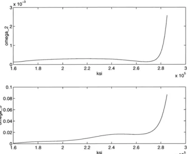
2-17 w, and wo₀as a function of . ... 42

2-18 Simulation block diagram for 2-nd order longitudinal dynamics . . . . 43

2-19 Root locus variation for 2-nd order longitudinal dynamics ... 44

2-20 Variable a time response for 2-nd order longitudinal dynamics . . . . 45

2-21 Variable & time response for 2-nd order longitudinal dynamics . . . . 45

2-22 Variable a time response for 2-nd order longitudinal dynamics . . . . 46

2-23 Variable & time response for 2-nd order longitudinal dynamics . . . . 46

2-24 Sensitivity of 2-nd order longitudinal dynamics to Cma ... ... 49

2-25 Sensitivity of 2-nd order longitudinal dynamics to CL, . . . . . 49

2-26 Sensitivity of 2-nd order longitudinal dynamics to Cm, ... ... 50

2-27 Sensitivity of 2-nd order longitudinal dynamics to Cdo . . . . 50

2-28 Sensitivity of 2-nd order longitudinal dynamics to CLo . . . . 51

(8)

2-30 Neural Network Model for 2nd order GHAME . . . . 2-31 Neural Network Model for 2nd order GHAME with 10% uncertainty . 2-32 Neural Network Model for 2nd order GHAME with 20% uncertainty . 2-33 Damping Coefficient wl ( ) with

+20%

uncertainty . . . .

2-34 Neural Network Model for 2nd order GHAME with 15% increase in

W 1 ( ) . . . .

2-35 Neural Network Model for 2nd order GHAME with 20% increase in

W 1() . . . .. . .

3-1 Stability derivative D. and D, as a function of . . . .

3-2 Stability derivative L. and L, as a function of . . . .

3-3 Stability derivative M, and Mq as a function of . . . .

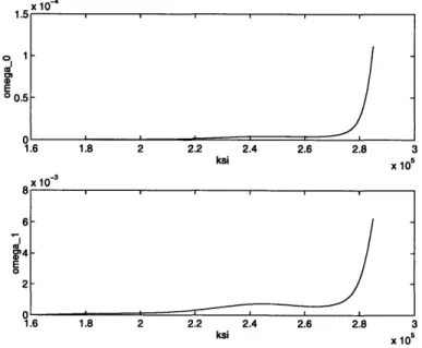
3-4 Time-varying coefficient wo and wl as a function of . . . .

3-5 Time-varying coefficient w2 and w3 as a function of . . . .

3-6 Simulation block diagram for 4-th order longitudinal dynamics . . . .

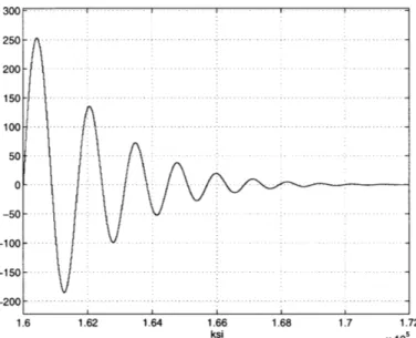
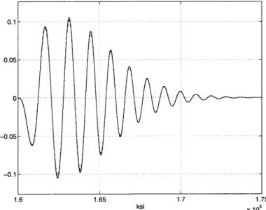
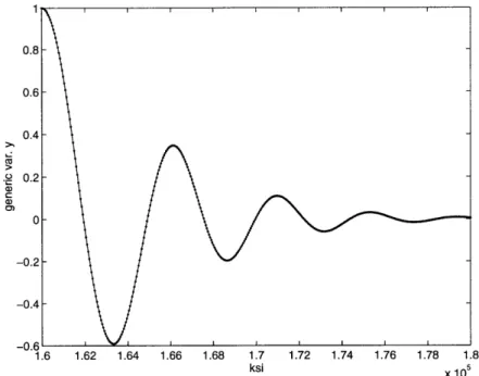
3-7 Root locus variation for 4-th order longitudinal dynamics . . . . 3-8 Root locus variation for 4-th order longitudinal dynamics . . . . 3-9 Time response of y for 4th order longitudinal dynamics . . . . 3-10 Time response of y' for 4th order longitudinal dynamics . . . . 3-11 Time response of y for 4th order longitudinal dynamics . . . . 3-12 Time response y' for 4th order longitudinal dynamics . . . . 3-13 Time response of y for 4th order longitudinal dynamics . . . . 3-14 Time response y' for 4th order longitudinal dynamics . . . . 3-15 Time response of y for 4th order longitudinal dynamics . . . . 3-16 Time response y' for 4th order longitudinal dynamics . . . . 3-17 Sensitivity of 4th order longitudinal dynamics to D . . . .

3-18 Sensitivity of 4th order longitudinal dynamics to D . . . . 3-19 Sensitivity of 4th order longitudinal dynamics to L . . . . 3-20 Sensitivity of 4th order longitudinal dynamics to L . . . .

3-21 Sensitivity of 4th order longitudinal dynamics to Ma . ...

3-22 Sensitivity of 4th order longitudinal dynamics to Mq . . . . .

3-23 Neural Network Model for 4th order GHAME . . . . 3-24 Neural Network Model for 4th order GHAME . . . . 3-25 Neural Network Model for 4th order GHAME with 10% uncertainty 3-26 Neural Network Model for 4th order GHAME with 20% uncertainty 3-27 Damping Coefficient wl ( ) with ±20% uncertainty . . . .

3-28 Neural Network Model for 4th order GHAME with 10% uncertainty 3-29 Neural Network Model for 4th order GHAME with 20% uncertainty 4-1

4-2 4-3 4-4

Aerodynamic coefficient CY as a function of M and a. Aerodynamic coefficient CI, as a function of M and a Aerodynamic coefficient C1, as a function of M and a . Aerodynamic coefficient C1, as a function of M and a .

viii 54 54 55 55 56 56 60 60 60 62 63 64 65 65 66 66 67 67 68 68 69 69 71 71 72 72 73 73 74 75 76 76 77 77 78 81 82 82 83 . . . . v

(9)

4-5 Aerodynamic coefficient C,, as a function of M and a . ... 83

4-6 Aerodynamic coefficient C,, as a function of M and a . ... 84

4-7 Aerodynamic coefficient C,r as a function of M and ca . ... 84

4-8 Stability derivative Y, and L, as a function of ( . ... 87

4-9 Stability derivative L, and LP as a function of . ... 87

4-10 Stability derivative N,, Np and Nr as a function of . ... 88

4-11 Time-varying coefficient wo and w1 as a function of . ... 88

4-12 Time-varying coefficient w2 and w3 as a function of ( . ... 89

4-13 Simulation block diagram for 4-th order lateral-directional dynamics . 89 4-14 Root locus variation for 4-th order lateral-directional dynamics . . . . 91

4-15 Root locus variation for 4-th order lateral-directional dynamics . . . . 91

4-16 Time response of y for 4th order lateral-directional dynamics .... . 92

4-17 Time response y' for 4th order lateral-directional dynamics ... 92

5-1 Root locus variation for 3rd order VTOL longitudinal dynamics . . . 98

5-2 Root locus variation for 3rd order VTOL longitudinal dynamics . . . 99

5-3 Simulation block diagram for perturbation variable u(t) and O(t) dy-namics of VTOL aircraft ... ... 100

5-4 Time response of u for 3rd order VTOL longitudinal dynamics model 101 5-5 Time response of i for 3rd order VTOL longitudinal dynamics model 102 5-6 Time response of u for 3rd order VTOL longitudinal dynamics model 102 5-7 Time response of it for 3rd order VTOL longitudinal dynamics model 103 5-8 Time response of 0 for 3rd order VTOL longitudinal dynamics model 104 5-9 Time response of 8 for 3rd order VTOL longitudinal dynamics model 104 5-10 Time response of 0 for 3rd order VTOL longitudinal dynamics model 105 5-11 Time response of 0 for 3rd order VTOL longitudinal dynamics model 105 5-12 Neural Network Model for 3rd order VTOL . ... 106

5-13 Neural Network Model for 3rd order VTOL with 10% uncertainty . 107 5-14 Neural Network Model for 3rd order VTOL with 20% uncertainty . 107 5-15 Coefficient c2 (t) with ±20% uncertainty . ... 108

5-16 Neural Network Model for 3rd order VTOL . ... 108

5-17 Neural Network Model for 3rd order VTOL with 10% uncertainty . 109 5-18 Neural Network Model for 3rd order VTOL with 15% uncertainty . 109 5-19 Neural Network Model for 3rd order VTOL with 20% uncertainty . 110 5-20 Root locus variation for 4th order VTOL longitudinal dynamics . . . 112

(10)

5-22 Root locus variation for 4th order VTOL longitudinal dynamics . . . 5-23 Root locus variation for 4th order VTOL longitudinal dynamics . . . 5-24 Time response of u for 4th order VTOL longitudinal dynamics model 5-25 Time response of it for 4th order VTOL longitudinal dynamics model 5-26 Time response of u for 4th order VTOL longitudinal dynamics model 5-27 Time response of it for 4th order VTOL longitudinal dynamics model 5-28 Sensitivity of 4th order VTOL longitudinal dynamics to X . . . . .

5-29 Sensitivity of 4th order VTOL longitudinal dynamics to Z . . . . .

5-30 Sensitivity of 4th order VTOL longitudinal dynamics to M . . . . .

5-31 Sensitivity of 4th order VTOL longitudinal dynamics to Z ...

5-32 Sensitivity of 4th order VTOL longitudinal dynamics to M . . . . . 5-33 Sensitivity of 4th order VTOL longitudinal dynamics to Mq . . . . .

6-1 N-feed-forward multilayer neural network, z- 1 - time shift operator Structure of backpropagation through time . . . .

System Identification Scheme . . . . Structure of Neural Networks Model . . . .

Neural Networks for an Online System Identification Neural Networks for an Online System Identification Neural Networks for an Online System Identification Neural Networks for an Online System Identification Neural Networks for an Online System Identification Neural Networks for an Online System Identification Neural Networks for an Online System Identification Neural Networks for an Online System Identification Variation of Stability Derivatives M . . . . Neural Networks for Online System Identification . . Indirect Adaptive Control ...

Result of IAC for VTOL during Transition . . . . IAC for VTOL during Transition ...

IAC for VTOL during Transition with change in Mu

. . . . . 124 . . . . . 128 . . . . . 128 . . . . . 131 . . . . . 132 . . . . . 133 . . . . . 134 . . . . . 135 . . . . . 136 . . . . . 137 . . . . . 138 . . . . 140 . . . . . 140 ... 142 . . . . . 144 ... 145 . . . . . 146

6-19 IAC for VTOL during Transition with change in M, and the presence of time lag ... 147

6-20 IAC for VTOL during Transition with change in Mu and noise in sensor148 6-21 SIMULINK block diagram for PI controller . ... 151

6-22 SIMULINK block diagram for adaptive control . ... 152

6-23 PI Control for VTOL during Transition . ... . . . . 153

6-24 PI Control for VTOL during Transition with change in Mu ... 154

6-25 Adaptive Control for VTOL during Transition with change in M' . . 155

6-26 Adaptive Control for VTOL during Transition with change in Mu and tim e lag . . . ... 156 114 114 115 115 116 116 118 119 119 120 120 121 123 6-2 6-3 6-4 6-5 6-6 6-7 6-8 6-9 6-10 6-11 6-12 6-13 6-14 6-15 6-16 6-17 6-18

(11)

6-27 Adaptive Control for VTOL during Transition with change in M" and noise in the sensor system . . . . . . . . ..

A-1 A-2 A-3 A-4 A-5 A-6 A-7 A-8 A-9 A-10 A-11 A-12 A-13 A-14 A-15 A-16 A-17 A-18 A-19 A-20 A-21 A-22 A-23 A-24 A-25 A-26 A-27 A-28 A-29 A-30 A-31 A-32 Aerodynamics Aerodynamics Aerodynamics Aerodynamics Aerodynamics Aerodynamics Aerodynamics Aerodynamics Aerodynamics Aerodynamics Aerodynamics Aerodynamics Aerodynamics Aerodynamics Aerodynamics Aerodynamics Aerodynamics Aerodynamics Aerodynamics Aerodynamics Aerodynamics Aerodynamics Aerodynamics Aerodynamics Aerodynamics Aerodynamics Aerodynamics Aerodynamics Aerodynamics Aerodynamics Aerodynamics Aerodynamics coefficient coefficient coefficient coefficient coefficient coefficient coefficient coefficient coefficient coefficient coefficient coefficient coefficient coefficient coefficient coefficient coefficient coefficient coefficient coefficient coefficient coefficient coefficient coefficient coefficient coefficient coefficient coefficient coefficient coefficient coefficient coefficient

B-i Aerodynamics coefficient CLLB as a function of angle of attack a and Mach number M ....

B-2 Aerodynamics coefficient Mach number M .... B-3 Aerodynamics coefficient

Mach number M . . . .

CLLDA as a function of angle of attack a and

..CLL as a function of ... angle of at...tack a an...

CLLDR as a function of angle of attack a and

CMO as a function of angle of attack a . . . CMO as a function Mach number M . . . . .

CMA as a function of angle of attack a . . .

CMA as a function Mach number M . . . .

CLO as a function of angle of attack a . . . CLO as a function Mach number M . . . . . CLA as a function of angle of attack a . . . CLA as a function Mach number M . . . . . CDO as a function of angle of attack a . . .

CDO as a function Mach number M . . . . .

CDA as a function of angle of attack a . . . CDA as a function Mach number M . . . . .

CLL, as a function of angle of attack a . . . CLLB as a function Mach number M . . . .

CLLDA as a function of angle of attack a . .

CLLDA as a function Mach number M . . . CLLDR as a function of angle of attack a . . CLLDR as a function Mach number M . . . . CLLP as a function of angle of attack a . . .

CLLP as a function Mach number M . . . .

CLLR as a function of angle of attack a . . . CLLR as a function Mach number M . . . .

CLN as a function of angle of attack a . . .

CLN,, as a function Mach number M . . . .

CLNDA as a function of angle of attack a . . CLNDA as a function Mach number M . . . CLNDR as a function of angle of attack a . .

CLNDR as a function Mach number M . . . CLNP as a function of angle of attack a . . . CLNP as a function Mach number M . . . .

CLNR as a function of angle of attack a . . . CLNR as a function Mach number M . . . .

157 167 168 169 170 171 172 173 174 175 176 177 178 180 181 182 183 184 185 186 187 188 189 191 192 193 194 195 196 197 198 199 200 202 203 204

(12)

B-4 Aerodynamics coefficient CLLP as a function of angle of attack a and Mach number M ... . . ... ... 205 B-5 Aerodynamics coefficient CLLR as a function of angle of attack a and

Mach number M ... .... .. ... .. 206 B-6 Aerodynamics coefficient CLNB as a function of angle of attack a and

Mach numberM ... .. ... ... ... 207 B-7 Aerodynamics coefficient CLNDA as a function of angle of attack a and

Mach number M ... ... .. ... . 208 B-8 Aerodynamics coefficient CLNDR as a function of angle of attack a and

Mach number M ... . ... ... .. 209 B-9 Aerodynamics coefficient CLNP as a function of angle of attack a and

Mach number M ... . ... ... .. 210 B-10 Aerodynamics coefficient CLNR as a function of angle of attack a and

Mach number M ... ... 211 B-11 Aerodynamics coefficient CLo as a function of angle of attack a and

Mach number M ... . . ... ... .. 212 B-12 Aerodynamics coefficient CLA as a function of angle of attack a and

Mach number M ... ... .... 213 B-13 Aerodynamics coefficient CDo as a function of angle of attack a and

Mach number M ... .... .. . ... 214 B-14 Aerodynamics coefficient CDA as a function of angle of attack a and

Mach number M .... ... . ... .. .. 215 B-15 Aerodynamics coefficient CMo as a function of angle of attack a and

Mach number M ... ... .. 216

B-16 Aerodynamics coefficient CMA as a function of angle of attack a and Mach number M ... . ... ... . 217

C-1 Aerodynamics coefficient CLLB as a function of angle of attack a and

Mach number M : exact versus 2-D polynomial approximation . . . . 219

C-2 Aerodynamics coefficient CLLDA as a function of angle of attack a and

C-3 Aerodynamics coefficient CLLDR as a function of angle of attack a and

C-4 Aerodynamics coefficient CLLP as a function of angle of attack a and

C-5 Aerodynamics coefficient CLLR as a function of angle of attack a and

C-6 Aerodynamics coefficient CLNB as a function of angle of attack a and

C-7 Aerodynamics coefficient CLNDA as a function of angle of attack a and

(13)

C-8 Aerodynamics coefficient CLNDR as a function of angle of attack a and Mach number M : exact versus 2-D polynomial approximation .... 226 C-9 Aerodynamics coefficient CLNp as a function of angle of attack a and

Mach number M : exact versus 2-D polynomial approximation .... 227 C-10 Aerodynamics coefficient CLR as a function of angle of attack a and

Mach number M : exact versus 2-D polynomial approximation .... 228

C-11 Aerodynamics coefficient CLo as a function of angle of attack a and

Mach number M : exact versus 2-D polynomial approximation .... 229 C-12 Aerodynamics coefficient CLA as a function of angle of attack a and

Mach number M : exact versus 2-D polynomial approximation .... 230 C-13 Aerodynamics coefficient CDo as a function of angle of attack a and

Mach number M : exact versus 2-D polynomial approximation .... 231 C-14 Aerodynamics coefficient CDA as a function of angle of attack a and

Mach number M : exact versus 2-D polynomial approximation .... 232 C-15 Aerodynamics coefficient CMo as a function of angle of attack a and

Mach number M : exact versus 2-D polynomial approximation .... 233 C-16 Aerodynamics coefficient CMA as a function of angle of attack a and

Mach number M : exact versus 2-D polynomial approximation .... 234

(14)

List of Tables

1.1 A historical sketch of ANN research as part of soft computing evolution

[4] . . . . 4

1.2 Neural networks as a constituent of soft computing [4] ... . 6

1.3 Activation function for neuron ... ... 14

2.1 Stability derivatives ... ... ... . 32

5.1 VTOL Stability Derivatives ... 97

6.1 Mean Square Error comparison for different learning rates ... 129

6.2 Mean Square Error comparison for different number of hidden neurons 129 6.3 Mean Square Error comparison for different activation function . . . . 130

6.4 Error Comparison (No change in parameters) . ... 152

6.5 Error Comparison (change in M,) ... 152

7.1 Some of advantages and disadvantages of using ANN for AFCS . . .. 162

(15)

Nomenclature

ABBREVIATIONS

AFCS Automatic Flight Control System AI Artificial Intelligent

ANN Artificial Neural Networks BITE Built In Test Equipment

FDIE Fault Detection and Isolation Equipment

GHAME Generic Hypersonic Aerodynamic Model Example IAC Indirect Adaptive Control

LEO Low-Earth-Orbit LTI Linear Time Invariant LTV Linear Time Varying

NNC Neural Networks Controller NNM Neural Networks Model

MRAC Model Reference Adaptive control MSE Mean Square Error

PI Proportional Integral SSTO Single-Stage-to-Orbit

SSV Single Stage-Orbiter Vehicle STOL Short TakeOff and Landing TPS Thermal Protection System VTOL Vertical TakeOff and Landing

GENERAL NOMENCLATURE

x Time derivative of x

x' Derivative with respect to (

x Estimate of x

Ax Discrete difference in x

(16)

NEURAL NETWORK NOMENCLATURE

Neuron activation function Number of input neurons Number of output neurons

Total number of neurons in the networks Input neuron(s)

Output neuron(s)

Hidden neurons

Neuron i, layer j input signal Neuron i, layer j activation level Weight connecting neurons i and k

Neuron i in in layer j, neuron k is in layer j - 1 learning rate

AIRCRAFT DYNAMICS NOMENCLATURE

Speed of sound Reference span Reference chord Drag Span efficiency Gravitational acceleration Altitude

Wing tilt angle Moments of inertia Radii of gyration

Lift, in longitudinal equations

Rolling moment, in lateral-directional equations Mach number

Pitching moment, in lateral-directional equations

xvi

f (x)

m n N+n

Xi

i Xi Xj,i Yj,i Wj,ixk a b C D e g h i

Ix,

ly,

IIzz, Ixz kx, ky, kz

L M

(17)

Yawing moment Mass of the aircraft Roll rate

Pitch rate Yaw rate

Radial distance from center of the Earth Reference area

Absolute temperature

Thrust, in longitudinal equations

Perturbation velocity in x, y, z direction Flight speed

Weight

Generic variable Angle of attack

Side-slip angle

Nondimensional mass of atmosphere Control deflection

Subscript 'N':

e: elevator r: rudder T: thrust

Gradient of atmosphere absolute temperature Flight path angle

Ratio of moment of inertia Air mass density

Inverse nondimensional pitching moment of inertia Euler angle, roll

Euler angle, pitch Euler angle, yaw

Vehicle lengths along trajectory

xvii U, V, V W y a 6N

Ps

(18)

Chapter 1 Introduction to Neural Networks

The ubiquity of the concept, design and application of intelligent systems in recent years has displayed signs that the approach to the engineering problems has changed. People are attempting to forge biologically-inspired methods into many aspects of engineering problems. Those efforts are focused on the exploration of human-like systems typified by some distinct features not found in traditional logic. Much of en-gineering today is still based on the knowledge of unchanging objects where decisions are made largely from facts. This is safe and -at times- accurate. But it hinders creativity and thus the horizon of new potential; as well as being inadequate logic sys-tem for certain problems, particularly ones which involve uncertainties, time-varying or unknown parameters.

Presently we have the requisite hardware, software and sensor technologies at our disposal for assembling intelligent systems. All the progress owes to the evolution of computing methodologies -as the backbone of such systems- dating back to the 1940s when the first neuron model was devised by McCulloch and Pitts. Neural networks is one of the main constituents of modern computing methodology; the other ones being the fuzzy set theory and genetic algorithm/simulated annealing.

Neural networks innovate the realm of information processing and computation with its distinct feature of learning and adaptation. The method is based on the biological process in the human brain. The brain as a source of natural intelligence has both strengths and weaknesses compared to modern computer. It process incomplete information obtained by perception at an incredibly rapid rate. Nerve cells function about 106 times slower that electronic circuit gates, but human brain processes visual and auditory information much faster than modern computers [4]. Neural network methods explore the brain internal mechanism to simulate its powerful functionality. A neural network is a nonalgorithmic computation technique in which the con-nectionist architecture of the brain is simulated with a continuous-time nonlinear dynamic system to mimic intelligent behavior. Such connectionism substitutes sym-bolically structured representations with distributed representations in the form of weights between a massive set of interconnected neurons (or processing units) and a

(19)

CHAPTER 1. INTRODUCTION TO NEURAL NETWORKS

surprisingly simple processor. It does not need critical decision flows in its 'algorithm'. We do not need to have a detailed process to algorithmically convert an input to an output. Rather, all that one need for most networks is collection of representative examples of the desired translation. The power of an artificial neural network (ANN) approach lies not necessarily in the elegance of the particular solution, but rather in the generality of the networks to find its own solution to particular problems, given only instances of the desired behavior.

As a novel computing methodology, neural networks approach is aimed at solving real-world decision making, modeling and control problems. One area of particular significance is system identification and control system design for aerospace vehicles whereby some or all of the pilot's ability is replaced or augmented. During its evo-lution in the past neural networks have not been used as an acceptable possibility since engineers prefer to use well-defined systems due to the stringent requirement of safety. That is one of the reasons why linear control has occupied large areas in the engineering systems. A certain class of (flight) dynamics problems represents a complex behavior characterized by:

L Nonlinear dynamics

[l Unknown parameters or uncertainties

OL Time-varying parameters in vehicle plant and environment

l Time lags

ol Noise inputs from sensors and from air disturbances

Conventional technology could not in general cope with most of these problems. The use of neural networks provides a potential method by which the problems can be approached, analyzed and overcome.

1.1 Basic Perspective of Neural Networks

1.1.1 Definition and Remarks

What are neural networks? There have been numerous definitions that is represen-tative in describing the ANN. Some conceptual as well as technical notions from researchers are listed below.

A neural network is a parallel, distributed information processing struc-ture consisting of processing elements (which can posses a local memory

(20)

and carry out localized information processing operations) interconnected together with unidirectional signal channels called connections. Each pro-cessing element has single output connection which branches ('fans out') into as many collateral connections as desired (each carrying the same signal - the processing element output signal). The processing element output signal can be of any mathematical type desired. All of the pro-cessing that goes on with each propro-cessing element must be completely local i. e., it must depend only upon the current values of the input signal arriving at the processing element via impinging connections and upon values stored in the processing element's local memory [13]

Artificial neural networks are methods of computing that are designed to exploit the organizational principles that are felt to exist in biological neural systems [12].

Neural networks are massively parallel systems that rely on dense arrange-ments of interconnections and surprisingly simple processors [10].

Neural networks are self-organizing information systems in which infor-mation organizes itself [9].

Those attributes illustrate the novelty of neural networks in contrast to traditional computing and information systems. It is the self-organizing characteristic resulting solely from its internal dynamics that gives neural networks great capabilities.

1.1.2 Milestones on Neural Networks Research

Artificial neural networks method is still sometimes referred as new method though it has evolved for more than 50 years along with other 'soft' computing constituents (see Table 1.1). The list below gives the brief historical notes on neural networks research.

O 1943. W. McCulloch and W.Pitts designed the first neuron model. Their paper

- _{"A Logical calculus of the ideas immanent in nervous activity"- presents}

the mathematical formalization of a neuron, in which a weighted sum of input signals is compared to a threshold to determine wheter or not the neuron fires. It shows that simple neural networks can compute any arithmetic or logical function.

oE 1948. Weiner's seminal book Cybernetics posed that cybernetics as the study

(21)

Table 1.1: A historical sketch of ANN research as part of soft computing evolution [4]

Year Conventional ANN Fuzzy systems Other methods AI

1940s 1947. 1943

Cybernetics McCulloch -Pitts neuron model 1950s 1956. Artificial 1957.

Intelligence Perceptron

1960s 1960. Lisp 1960s Adaline/ 1965. Fuzzy Language Madaline sets

1970 mid-1970s. 1974. Birth. 1974. Fuzzy 1970s. Genetic Knowledge En- of backpropaga- controller Algorithm gineering (Ex- tion algorithm.

pert systems) 1975. Cognitron and

Neocognitron

1980 1980. Self- 1985 Fuzzy mid-1980s Ar-organizing map. modeling tificial life Im-1982. Hopfield mune modeling Net. 1983 Boltzmann machine. 1986 Backpropa-gation algorithm boom 1990 1990. Neuro- Genetic

fuzzy modeling. programming 1991. ANFIS.

(22)

sciences, control and neurobiology. As we know today, those constituents have tended to go their own separate ways and at times creates a barrier to effective interchange of ideas between the disciplines.

E 1949. D. O. Hebb introduced a important learning method in his book The

Organization of Behavior which is used in some form in most learning rules

used today. The major proposal of this book is that behavior can be explained by the neuron activities.

O 1951. Minsky and Edmonds devised the first hardware realization of a neural network.

O 1958. F. Rosenblatt presented the first practical ANN called perceptron, a basic unit for many other ANN. A form of Hebbian learning rules were used in the learning techniques for perceptron.

O 1960. B. Widrow and M.E. Hoff introduced an adaptive perceptron-like network that can learn quickly and accurately. Known today as Adaline, the system has inputs and a desired output classification for each input. The well-known gradient descent method is used to minimize the least mean square error as for weights adjustment rules.

OE 1969. M. Minsky and Seymour Papert caused widespread pessimism -causing

inhibition of research funding and activities for several years- among the ANN researches with their book Perceptrons. The book rigorously describes the limi-tation of perceptron learning capability and is closed with the remark that field of ANN is a dead end. Though this has been proved to be not entirely true, the premise has showed the kind of problems that can or can not be solved by perceptron.

o 1972. Teuko Kohonen and J. A. Anderson worked independently to come to

closely related results. Kohonen proposed a correlation matrix model for as-sociative memory, while Anderson did for a 'linear associator' for the same purpose. A generalized Hebbian learning rules were used to correlate input and output vectors. While Kohonen's work gave emphasize on mathematical structure, Anderson's remarks put weight on physiological plausibility of the network.

Ol 1974. P.J. Werbos brought new ideas in error minimization algorithm of ANN

learning rules. His Ph.D. thesis "Beyond regression: new tools for prediction and analysis in the behavior sciences" was published and gave birth to a now famous learning rule - backpropagation.

(23)

CHAPTER 1. INTRODUCTION TO NEURAL NETWORKS 6

Table 1.2: Neural networks as a constituent of soft computing [4] Methodology Strength

Neural network Learning and adaptation Fuzzy set theory Knowledge representation

via fuzzy if-then rules Genetic algorithm and sim- Systematic random search ulated annealing

Conventional artificial Symbolic manipulation intelligence

L 1976. S. Grossberg proposed a self-organizing neural network. The idea was based on the visual system. The network is characterized by internal continuous-time competition. This gives the basis for concepts of the adaptive resonance theory (ART) networks.

O 1982. J.J. Hopfield, in his paper "Neural networks and physical systems with

emergent collective computation abilities", described a content-addressable neu-ral network. This recurrent networks (today called Hopfield Net) was considered highly influential in bringing about the renaissance of neural network research that year.

At present research on neural networks is still growing. Some of it is still directed to the learning method refinement (that once caused backpropagation algorithm boom in the late 1980's). On the other side, people have tended to resort to the idea of cybernetics where computation, information systems, control and neurobiology meet. This tendency has created a new discipline called 'soft computing' consisting a mix of the separated fields. In this discipline neural network method has blended with the other methodologies: fuzzy logic, probabilistic reasoning and genetic algorithm. Each of the elements has its own distinction. So they are complementary rather than competitive with each other. The significant contribution of neural networks is

methodology for system identification, learning and adaptation; that of fuzzy logic is computing with words; that of probabilistic reasoning is propagation of belief; and that of genetic algorithm is systematized random search and optimization. Table 1.2

enumerates the strength of each soft computing elements.

Along with the unfolding of the neural networks research, industry has responded with various applications in different fields ranging from consumer electronics and industrial process control to decision support systems and financial trading. With

(24)

many real-world problems that are imprecisely defined, contain uncertainties and require human intervention, neural networks method is likely to play an increasingly important roles today and in the future.

1.2 The Characteristics of Neural Networks

There are many reasons why neural networks are a likely candidate for an attractive new design of system identification and control of aerospace vehicles. They stem from ANN's intrinsic properties; they are summarized below from various references.

Ol Potential of intelligent and natural control. Inspired by biological neural

networks, ANN are employed to deal with pattern recognition, and nonlinear regression and classification problems. It can also imitate human behavior if desired.

[l Real-time parallel processing. Neural networks have a highly parallel

struc-ture which lends itself immediately to parallel implementation. Such an imple-mentation can be expected to achieve a higher degree of fault tolerance than conventional schemes. The basic processing element in a neural network has a very simple structure. This, in conjunction with parallel implementation, results in very fast overall processing.

O Nonlinear systems. Neural networks have the greatest promise in the realm

of nonlinear control problems. This emanates from their theoretical ability to approximate arbitrary nonlinear mappings. These networks are likely to also achieve more parsimonious modelingthan alternative approximation schemes.

O Resistance to noisy data. This capability comes from its ability to learn a

general pattern not necessarily an exact figures.

O Multivariable System. Neural networks naturally process many inputs and

have many outputs; they are readily applicable to multivariable systems.

Ol Computational efficiency. Without assuming to much background

knowl-edge of the problem being solved, neural networks rely heavily on high-speed number-crunching computation to find rules or regularity in data sets. This is a common feature of all areas of computational intelligence.

LO Fault Tolerance. The structure of neural networks depicts its inherent fault

tolerance characteristic. ANN architectures encode information in a distributed fashion. Typically the information that is stored in neural networks is shared

(25)

by many of its processing elements. This kind of structure provides redundant information representation. The deletion of some neurons does not necessarily destroy the system. Instead, the system continues to work with gracefully de-graded performance; thus the result is a naturally fault -or error- tolerant system.

o Quickly integrated into systems. Control systems using neural networks,

for example, has fixed software/hardware architecture. Changing the control algorithm amounts to changing the weights of the neural connections and not the structure of the controller.

O No requirement of explicit programming. Neural networks are not

pro-grammed; they learn by example. Typically, a neural network is presented with a training set consisting of a group of examples from which the network can learn. The training set, in the form of input-output value pairs is known as the patterns. The absence of human development of algorithms and programs suggests that time and human effort can be saved.

ol The ability of universal approximation. The nonlinear activation function

gives the neural network the capability of forming any nonlinear functional rep-resentation. It should be noted that there are other universal approximation methods. For example Taylor series, which use polynomial approximation and Fourier series, which use the sine and cosine trigonometric functions to approx-imate any continuous function. This ability is particularly useful in the case when internal dynamics of a system under study are not clear, unavailable, or nonlinear.

l Associative memory. The information in neural networks is stored in

as-sociative memory in contrast to digital computer's addressed memory where particular pieces of information are stored in particular locations of memory. This, besides giving a fault-tolerant property, is used to generalize between training examples.

Note that all of these characteristics of neural networks can be clarified through the simple mathematical structure of a neural networks model. Though the broad behavioral terms such as learn, generalize and adapt are used, the neural network behavior is simple and quantifiable at each node. In short, their internal mechanism is clear and tractable, but produces complex macroscopic behavior.

(26)

1.3 Artificial Neural Networks Applications in

Aerospace Engineering

There have been numerous research on ANN applications in aerospace field. There are at least two major reasons why bringing new technology is attractive. Firstly, per-formance gain over conventional approach is desirable; and secondly novel approaches can engender wider horizon of possibilities. Several key considerations driving ANN application to aerospace have been elaborated in the previous section dealing with ANN characteristics.

Universities, aircraft companies and research centers have been involved in the research of ANN for use in aerospace thus far. Some of them are summarized as follows:

L Flight Control. Jorgensen and Schley (1990) propose the use of ANN in

autolanding systems, to increase the operational safety envelope and provide methods of exploring alternative control systems capable of dealing with tur-bulent, possibly nonlinear control conditions. The method used was to set up a neural network to copy pilot's actions and hence attempt to obtain 'flight sense'.

O FDIE and BITE. Notable work in the area of Fault Detection and Isolation

Equipment (FDIE) as well as Built In Test Equipment (BITE) was published by Barron et al. (1990), where ANN were used successfully in the development of an FDIE and BITE system for an aircraft with reconfigurable flight controls.

l Pilot Aid. Numerous researchers have been used ANN in developing pilot

aids, for example in pilot decision support systems (Seidman 1990); and flight management systems (Burgin & Schnetzler 1990).

Ol Image Recognition. ANN have been used for image processing as well as

recognition, with application to identification of aircraft from visual or radar signals. Research in this area is abundant, and is described as a typical appli-cation of ANN (Freeman & Skapura 1991).

Ol Manufacturing. ANN are being investigated for use in process optimization

and control by several major aerospace company.

In the realm of control of aircraft or spacecraft, ANN will function either as the following roles [33]:

Controller. An ANN controller would perform mappings of state variables (as input

(27)

Critic. The critic networks can be trained to monitor to aircraft's dynamic state,

mission profile and hence evaluate system performance. Information from this critic can then be used to adapt a conventional adaptive controller or a Neu-ral Networks Controller (NNC). Pattern classification networks would then be suitable for this function.

Gain programmer. An ANN can be used as a gain scheduler/programmer, to link

with a conventional controller, under adaptive learning or static programming. This technique has many advantages since by limiting the output gain range, the Automatic Flight Control System (AFCS) can have 'proven' stability using conventional linear stability analysis techniques.

Monitoring, fault detection. A suitable application for ANN in AFCS is in

mon-itoring systems and Fault Detection and Isolation Equipment (FDIE). This is because ANN generally have a good fuzzy knowledge ability, can operate well with noisy data, and have good generality.

Plant mimic. Of perhaps more use in the design of conventional and modern

con-trollers, an ANN can be used to model plant (e.g. aircraft/spacecraft, envi-ronment, pilot) in order to optimize performance, find system inverse, dynamic derivatives, etc.

Not only could an ANN function as a mimic of the plant, which is really in the system identification role, but a network could be set up to model a reference plant with desired properties for a model reference adaptive controller (MRAC). This is however not recommended since for MRAC type systems it is customary to choose a reference model with well known properties: such as a linear model

1.4 Neural Networks Architecture

The network architecture is defined by the basic processing elements and the way in which they are interconnected. The basic processing element of the ANN architecture is often called a neuron, but other names such as unit, node, perceptron and adaline are also used. The neurons are connected by weights, also referred to as connections or

synapses, which convey the information. Neurons are also often collected into groups

called layers or slabs within which the neurons have a similar function or structure. Depending on their function in the net, one can distinguish three types of layers. The layers whose activations are input receptive for the net are called input layers, similarly layers whose activations represent the output of the net, output layers. The

(28)

INTRODUCTION TO NEURAL NETWORKS input layer hidden layer output layer

Figure 1-1: A Neural network structure with 2 hidden layers

In general, there can be any number of layers, and neurons in any layer can be connected to neurons in any other layer. Some neurons have no input from other neurons, and are known as bias, or threshold, unit. The memory content or signal strength of neuron is referred to as the activation level. Usually, the activation levels of the input and output units are scaled such that the activation levels are appropriate to neuron function and the observable values are given a physical meaning.

1.4.1 Neuron Model and Network Structure

Let us consider a single neuron from the networks structure which is depicted in Fig. 1-1. An individual neuron has many inputs, dependent on the number of incoming connections. Each connection to the neuron has a weight associated with it. After the total neuron input signal is calculated, that is given by the sum of the product of

inputs and weights:

(29)

n

j

i - Wj,ixkYjl,k (1.1)

k=1

this signal is converted into an activation value through a functional relationship. The nonlinear processing power lies within this transfer function.

yj,i = f(xj,i) (1.2)

There is a wide class of arbitrary functions which can be used for some ANN. The commonly used functions are listed in Table 1.3

The output of the neuron is obtained from the activation value also through a functional relationship. The identity function is usually used in this step. In general, the selection of the function that is used in neural networks depends on the type of patterns (input-output value pairs). At present, the selection of activation function is more art than science and the subject of much research. The important point to remember is that any nonlinear function will provide network with the capability of representing any nonlinear functional mappings.

(30)

CHAPTER 1. INTRODUCTION TO NEURAL NETWORKS 13

y..

J,i yii =f(xj,) n

x

=

w

_y

j,i k= j,i x k y-1 x k

Neuron i

Layerj

w w w px Ij,i x 2 ji x n w j,i x n-1

Y

y

...

y

j-1,1 j-1,2 j-1,n-1 j-1,n

(31)

Table 1.3: Activation function for neuron

Function Expression Annotation

name

Sigmoidal f(z) = i This differentiable,

step-Function like, positive (bounded

by (0, 1)) function is the most commonly used ac-tivation function for neu-ral networks

Hyperbolic f(x) = tanh(x) = Its characteristics

resem-Tangent ble those of the sigmoid

except that it is zero-mean function bounded by(-1, 1)

Threshold f(x) = H(x) = > 0 It is also called

Heavi-0, a < 0_X_<0 _{side step function and is}

non-differentiable, step-like and positive.

Signum f(x) = sgn(x) = 0 It is nondifferentiable,

Function ' step-like and zero-mean.

Ramp f(x) = ax This unbounded function

Function/ can be

Linear Scaling useful in some particular

Function conditions. Note that it

(32)

INTRODUCTION TO NEURAL NETWORKS

-10 -8 -6 -4 -2 0 2 4 6 8 10

Figure 1-3: Activation functions

... Ramp function /linear function - Sigmoidal function

... _{Hyperbolic Tanh}

- Threshold /Sign function

in ANN neurons

(33)

1.4.2 Types of Artificial Neural Networks

There are in general three different architectures of ANN. Each of them exhibits a particular way of processing the information throughout the networks. Though all these networks can perform various tasks, each of them is generally well-suited only for a certain class of problem. Ref. [14] provides a rich array of networks that has been developed during recent years. They are listed under the corresponding rubric below.

Feedforward Networks

In these networks the output is computed directly from the input in one pass; no feed-back is involved. Included in this category are perceptron (multi-layer perceptron), linear associator and adaline. Feedforward networks are used for pattern recognition and for function approximation. Examples of application areas for function approx-imation are adaptive filtering and automatic control. Some feedforward (and their variant) networks are listed as the following:

* Radial Basis Networks (RBN). RBN may require more neurons than standard feed-forward backpropagation networks, but often they can be designed in a fraction of the time it takes to train standard feed-forward networks. The activation function used is called radial basis function. It has a maximum of 1 when its input is 0; and approaches 0 when its input approaches 00 or -oo. The RBN work best when many training vector are available.

* Adaptive Critic. This networks are generally used in the reinforcement learning controller (similar to direct control concepts of traditional adaptive control). In this scheme a neural network is used as a judgement network capable of differentiating between good performance and bad performance.

Competitive Networks

These types of networks are characterized by two properties. First, they compute some measure of distance between stored prototype patterns and the input pattern. Second, they perform a competition to determine which neuron represents the proto-type pattern closest to the input. In the competitive networks the protoproto-type patterns are adjusted as new inputs that are applied to the network. These adaptive networks learn to cluster the inputs into different categories.

(34)

Recurrent (Dynamic Associative Memory) Networks

As opposed to feedforward network, this type of network has feedback that associates stored data with input data. In other words, they are used as associative memories in which data is recalled in association with input rather than by an address. Hopfield network is an example of recurrent networks.

1.5 Learning Algorithm

Learning is one of the basic features of intelligence. The concept of learning machines comes from biological models. It is an effective self-modification of the organism that lives in a complex and changing environment. Learning is a directed change in knowledge structure that improves the performance [5]. This section describes different learning rules in the training of neural networks. The word training here means the process of minimization error between the networks output and the desired one. The discussion will be restricted to the supervised feedforward model which is so far the most tractable and most applied network model [6].

Learning rules govern the modification of connectivity as a function of experience in neural network. Various learning rules have been developed and today the research in that field is still active. Basically, most of the learning rules is inspired by Hebb's law. Thus, we begin with the overview of the Hebb's law. Note that the list is not intended as rigorous or comprehensive. Rather, it is given as a synopsis for introductory purposes. For a more complete list, the reader can see Ref. [14]

1.5.1 Hebb's Law [2]

Hebb's law is the fundamental psychophysical law of associative learning. It serves as both the basic law of psychology and artificial neural systems. The essence of Hebb's law is formulated as follows:

"If neuron A repeatedly contributes to the firing of neuron B, then A's efficiency in firing B increases"

The combination of Hebb's law and Grossberg's neural modeling theory explain the learning process in Pavlovian experiments:

When a dog is presented with food it salivates. When the dog hears a bell it does not salivate initially. But after hearing the bell simultaneously with presentation of food on several consecutive occasions, the dog is subsequently found to be salivate when it hears the bell alone.

(35)

In general terms, when a conditioned stimulus (such as bell) is repeatedly paired with an unconditioned stimulus (such as food) which evokes an unconditioned re-sponse (such as salivation), the conditioned stimulus gradually acquires the ability to evoke the unconditioned response.

Hestenes in ref. [5] concludes that the association strength between stimulus and response that psychologist infer from their experiments is a crude measure of the synaptic coupling strength between neurons in the central nervous system. The same can be said about all association among ideas and actions. Thus, the full import of Hebb's law is this:

"All associative (long-term) memory resides in synaptic connections of the central nervous system, and learning consists of changes in synaptic coupling strengths"

The strengthening of specific synapses within neural circuits is the most accepted theory for learning and memory in the brain.

1.5.2 Generalized Delta Rule

The learning process (training) begins when error between ANN and the desired output is obtained. The main problem of learning in the network with three or more layers is how to modify an inner or hidden layer. The first answer is unsupervised competitive learning, which generates useful hidden-unit connection. The second answer is to assume a hidden-unit connection matrix, on a priori grounds. The third possible way is the modification of the hidden units through the backpropagation error. The determination of error starts with the output units, and then propagates to the next hidden layer, until it reaches the input units. This kind of learning is called generalized Delta Rule.

1.5.3 Sigma-Pi Units

This learning algorithm is applied for more general form of multilayer perceptron called Sigma-Pi network. The net input is given by 7 wiIIailai2 ... aik where i indexes

the conjuncts impinging on unit j and ail, ai2, ... , aik are the k units in the conjunct. Thus, the net input to each neuron is equal to weighted sum of all signals impinging on that neuron, as well as weighted sum of selected products of these signals. The more elaborate usage of Sigma-Pi units includes:

- Gates; weighted connections

- Dynamically programmable networks in which the activation value of some units determine the function of other units

An approach to the use of neural network in the analysis of a class of flight vehicles

An Approach to the Use of Neural Network in the

Analysis of a Class of Flight Vehicles

by

Agus Budiyono

B.Eng., Bandung Institute of Technology (1992)

Submitted to the Department of Aeronautics and Astronautics

in partial fulfillment of the requirements for the degree of

Master of Science in Aeronautics and Astronautics

at the

MASSACHUSETTS INSTITUTE OF TECHNOLOGY

February 1998

@ Agus Budiyono, 1997. All rights reserved.

The author hereby grants to MIT permission to reproduce and

distribute publicly paper and electronic copies of this thesis document

in whole or in part, and to grant others the right to do so.

Author

...

Department of Aeronautics and Astronautics

December 26, 1997

Certified by...

Rudrapatna V. Ramnath

Adjunct Professor of Aeronautics and Astronautics

Thesis Supervisor

Accepted by.

Jaime Peraire

Associate Professor

Chairman, Departmental Committee on Graduate Students

17.

s

An Approach to the Use of Neural Network in the Analysis

of a Class of Flight Vehicles

by

Agus Budiyono

Abstract

Acknowledgement

Contents

List of Figures

+20%

List of Tables

Nomenclature

f (x)

Xi

ly,

Ps

Chapter 1

Introduction to Neural Networks

1.1

Basic Perspective of Neural Networks

1.1.1

Definition and Remarks

1.1.2

Milestones on Neural Networks Research

1.2

The Characteristics of Neural Networks

1.3

Artificial Neural Networks Applications in

Aerospace Engineering

1.4

Neural Networks Architecture

1.4.1

Neuron Model and Network Structure

y..

x

=

w

y

Neuron i

Layerj

Y

y

...

y

y

1.4.2

Types of Artificial Neural Networks

1.5

Learning Algorithm

1.5.1

Hebb's Law [2]

_y