An analysis of a diffusive-flux-limited model for groundwater cleanup rate estimation using air sparging

An Analysis of a Diffusive-Flux-Limited Model for

Groundwater Cleanup Rate Estimation Using Air Sparging

by

David F. Lockwood

S.B., Chemical Engineering

Massachusetts Institute of Technology, 1996

Submitted to the Department of Civil and Environmental Engineering In Partial Fulfillment of the Requirements for the Degree of

MASTER OF ENGINEERING

IN CIVIL AND ENVIRONMENTAL ENGINEERING at the

MASSACHUSETTS INSTITUTE OF TECHNOLOGY June 1997

@ 1997 David F. Lockwood

All rights reserved

The author hereby grants to MI. T permission to reproduce and distribute publicly paper and electronic copies of this thesis document in whole or in part.

Signature of the Author

David F. Lockwood

/ /57 May 9, 1997

Certified by

-- Chiang C. Mei

Edmund K. Turner Professor Civil and Enviroinmrental Engineering

') Thesis Supervisor

Accepted by

Professor Joseph Sussman :' Chairman, Department Committee on Graduate Studies

An Analysis of a Diffusive-Flux-Limited Model

for Groundwater Cleanup Rate Estimation Using Air Sparging

by

David F. Lockwood

Submitted to the Department of Civil and Environmental Engineering on May 9, 1997 in partial fulfillment of the requirements of the degree of

Master of Engineering in Civil and Environmental Engineering

Abstract

Air sparging (AS) is a remediation technology used in conjunction with soil/vapor extraction (SVE) to enhance the removal of volatile organic compounds (VOCs). Air sparging involves injection of air beneath the water table in the zone of contamination. VOCs are removed by two mechanisms: volatilization and biodegradation. As injected air moves through the subsurface and comes in contact with dissolved contamination or free product, VOCs volatilize and are removed with the rising air. Upon reaching the vadose zone, contaminated air is extracted by an SVE system and then treated before being released to the atmosphere. Injection of air also increases the amount of oxygen in the saturated zone which increases the rate of aerobic biodegradation.

Air sparging is a relatively new technology, and there is controversy as to whether air rises as discrete bubbles or in channels. Katherine Sellers and Robert Schreiber of Camp Dresser & McKee, Inc. developed a conceptual model to estimate the removal rate of VOCs from groundwater using air sparging. The model assumes bubble flow and considers removal by volatilization only. In this project, the model was modified to yield a more accurate remediation time estimate at Fuel Spill 12 (FS-12) at the Massachusetts Military Reservation (MMR) on Cape Cod. Tortuosity was accounted for, and specific diffusivities were calculated for different components of JP-4 jet fuel. The model was then modified to account for channel flow. Measured and estimated parameters were inputted into the two models. Results of the bubble model showed that approximately 10 years of air sparging would be required for benzene, toluene, ethylbenzene, and xylene (BTEX) concentrations to decrease to maximum contaminant levels (MCLs). A channel flow model was also developed and yielded remediation time estimates of approximately 800 years.

Thesis Supervisor: Professor Chiang C. Mei

Acknowledgments

Several people have supported me throughout the year and this support enabled me to complete my thesis while also keeping my sanity. I would now like to take the opportunity to thank them.

Ed Pesce and Bob Davis provided me with information on Fuel Spill 12. They

always responded to my requests for reports or data in a timely manner. Chiang Mei helped to shape my thesis and give me focus. His guidance was instrumental in helping to bring my thesis to completion. Dave Marks, Shawn Morrissey, Jackie and Muriel were a great source of encouragement. I would also like to thank my friends who helped me to take my mind off my thesis periodically.

Finally, I would like to thank my parents, Richard and Rosa Lockwood, and my brothers, Daniel and Eric, for providing me with love and support when I most needed it.

Table

of Contents

A B ST R A C T ... 2

ACKNOW LEDGM ENTS ... ... 3

TABLE OF CONTENTS ... ... 4

LIST O F FIG UR ES ... ... 5

LIST O F TA BLES ... ... 5

1. INTRO DUCTIO N ... ... 6

2. CONCEPTUAL BACKGROUND OF AIR SPARGING ... ... 10

2.1. INTRODUCTION ... ... 10

2.2. REMOVAL MECHANISMS ... ... 10

2.2. 1. Introduction ... ... 10

2.2.2. Stripping ... ... ... ... 10

2.2.2.1. Volatilization: Free Product Removal ... 11

2.2.2.2. Groundwater Stripping: Dissolved Contamination Removal ... ... ... 12

2.2.3. Biodegradation ... 13

2.3. A IR C HANN ELIN G ... ... 14

2.4. PHYSICAL SITE CONSTRAINTS ... ... 15

2.5. CONTROL OF FLOW ... ... ... 18

2.6. RADIUS OF INFLUENCE (ROI) ... 18

2.7. PILOT STUDIES ... 21

3. MODELING AIR SPARGING AT FS-12 ... ₂₃

3.1. INTRODUCTION... .. ... 23

3.2. DESIGN BASED ON PILOT STUDY, HYPERVENTILATE MODEL... ... 23

3.3. A CRITICAL REVIEW OF AN AIR SPARGING MODEL ... 29

3.3. 1. Assumptions of Sellers and Schreiber Model ... 29

3.3.2. Measured Parameters... ... 30

3.3.3. Estimated Parameters... .... ... ... 31

3.3.4. Description ofM odel...33

3.3.5. M odel Analysis ... ... ... ... 38

3.4. AIR CHANNELING APPLIED TO MODEL ... ... 43

4. RESULTS AND DISCUSSION ... ₄₈

5. CONCLUSIONS AND RECOMMENDATIONS ... ... 52

REFERENCES ... ... 54

APPENDIX ... ... ... 55

List of Figures

FIGURE 1-1: SCHEMATIC OF AIR SPARGING AND SOIL VAPOR EXTRACTION SYSTEMS ... 8

FIGURE 1-2: M M R PLUM E MAP... ... 9

FIGURE 2-1: VOLATILITY OF DIFFERENT PETROLEUM PRODUCTS ... 11

FIGURE 2-2: BUBBLE FLOW VS. CHANNEL FLOW... ... 16

FIGURE 2-3: CHANNELED FLOW IN THE SUBSURFACE. (JONES 1996; JOHNSON, 1994)... 17

FIGURE 2-4: EFFECT OF INJECTION PRESSURE ON AIR FLOW ... 20

FIGURE 3-1: RADIUS OF INFLUENCE OF SOIL VAPOR EXTRACTION WELLS... ... 26

FIGURE 3-2: LAYOUT OF AIR SPARGING WELLS SHOWING RADII OF INFLUENCE... 27

FIGURE 3-3: LAYOUT OF SOIL VAPOR EXTRACTION WELLS SHOWING RADII OF INFLUENCE ... 28

FIGURE 3-4: VOLUME OF INFLUENCE. ... 32

FIGURE 3-5: AREA OF INFLUENCE, F. ... 34

FIGURE 3-6: DIFFUSIVE DISTANCE IN BUBBLE FLOW ... 35

FIGURE 3-7: CHANNEL CROSS-SECTIONAL AREA AND DIFFUSIVE DISTANCE BETWEEN CHANNELS ... 45

FIGURE 3-8: AREA USED TO ESTIMATE CHANNEL DENSITY...46

FIGURE 4- 1: COMPARISON OF BENZENE CONCENTRATION PROFILES FOR BUBBLE FLOW AN D CHANNEL FLOW ... ... . ... 50

FIGURE 4-2: COMPARISON OF TOLUENE CONCENTRATION PROFILES FOR BUBBLE FLOW AND CHANNEL FLOW . ... ... 51

List of Tables TABLE 2-1: OXYGEN AVAILABILITY ... ... 14

TABLE 2-2: LIMITS TO THE USE OF AIR SPARGING ... 19

TABLE 2-3: PILOT TEST PARAMETERS ... ... 21

TABLE 2-4: SITE AND PILOT TEST DATA NEEDED FOR DESIGN. ... 22

TABLE 3-1: M EASURED RADIUS OF INFLUENCE... ... ... 24

TABLE 3-2: SUMMARY OF KEY DATA FOR AIR SPARGING... ... 25

TABLE 3-3: BREAK DOWN OF MAJOR COMPONENTS OF JP-4 JET FUEL ... ... 41

TABLE 3-4: MOLECULAR WEIGHT, DENSITY, AND DIFFUSION COEFFICIENTS OF BTEX ... 42

TABLE 3-5: MEASURED PARAMETERS FOR BUBBLE FLOW MODEL...42

TABLE 3-6: ESTIMATED PARAMETERS FOR BUBBLE FLOW MODEL ... 42

TABLE 3-7: MEASURED PARAMETERS FOR CHANNEL FLOW MODEL ... ... 46

TABLE 3-8: ESTIMATED PARAMETERS FOR CHANNEL FLOW MODEL... ... 47

TABLE 3-9: DIFFUSION COEFFICIENTS AND CHANNEL FLOW DECAY COEFFICIENTS FOR BTEX ... 47

TABLE 4-1: COMPARISON OF DECAY COEFFICIENTS FOR BUBBLE FLOW AND CHANNEL FLOW...48

TABLE 4-2: COMPARISON OF TERMINAL RISE VELOCITIES, BUBBLE AND CHANNEL RADII, AND DIFFUSIVE DISTANCE FOR BUBBLE AND CHANNEL FLOW... ...49

1.

Introduction

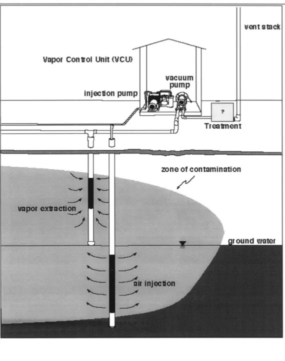
A developing technology that works in conjunction with soil vapor extraction (SVE) to facilitate the remediation of subterranean fuel spills is air sparging. Air

sparging is the injection of air into the saturated zone where contamination is present (see Figure 1-1). Air sparging removes fuel from the subsurface via two mechanisms:

stripping and biodegradation.

Soil vapor extraction (SVE) is a technology used in the remediation of subsurface contamination due to volatile organic compounds (VOCs). SVE involves the injection of fresh air into the vadose zone and the extraction of vapor via vacuum extraction wells. The idea behind SVE is to extract VOCs in the vapor phase, inducing more of the remaining liquid VOC to enter the vapor phase. The VOC vapor is then continuously extracted until remediation goals are met. Chapter 2 provides further explanation of the concepts behind air sparging.

Soil vapor extraction can be less costly than pump and treat for the removal of source contamination when contamination is far below the ground surface or when contaminants are highly volatile (contaminants whose vapor pressure is greater than 5 mm Hg and whose Henry's law constant is above 10-5 _atm-m3_mole-l_{) (Norris et al., 1994).}

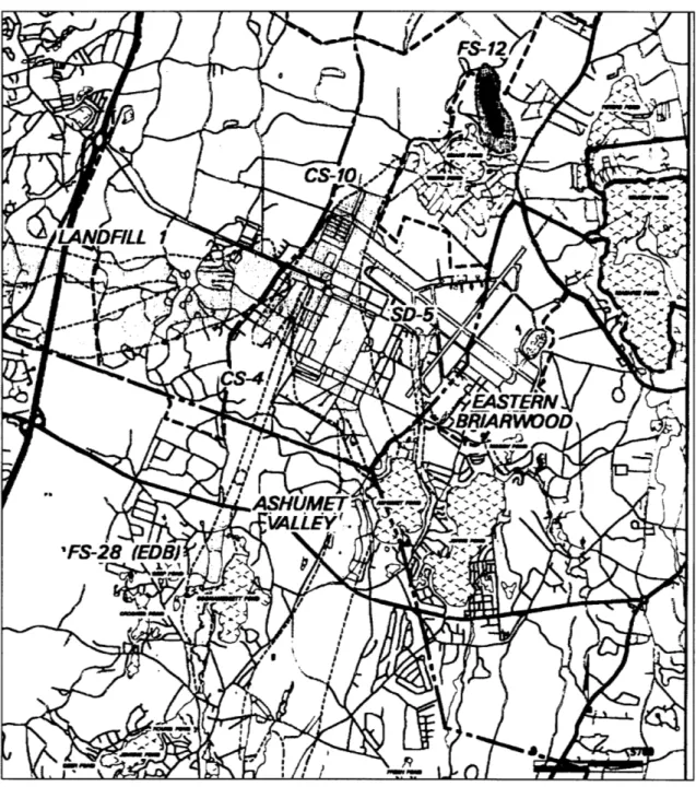
Both soil vapor extraction and air sparging are being used in the remediation of a fuel spill at the Massachusetts Military Reservation (MMR) on Cape Cod designated as Fuel Spill 12 (FS-12). FS-12 is one of several contamination plumes at the MMR (see Figure 1-2). FS-12 originated from a leak that occurred in an underground fuel pipeline between 1965 and 1972. An estimated 70,000 gallons of JP-4 jet fuel was spilled as a result of the leak.

The Fuel Spill 12 plume is located on the Upper Cape, near the top of the

Sagamore Lens. As the sole-source water-supply aquifer for western Cape Cod, the lens is of vital importance to the four towns adjacent to the MMR -Falmouth, Mashpee,

Sandwich, and Bourne (Ryan, 1980). Thus, it is essential that remediation goals are met to ensure that the groundwater is suitable for water supply.

As a preliminary design measure and due to cost considerations, it is necessary to estimate the groundwater cleanup rate. Katherine L. Sellers and Robert P. Schreiber of Camp Dresser & McKee (CDM) developed a conceptual model to estimate the rate of groundwater cleanup from the use of air sparging. In Chapter 3, the model is explained and estimated parameters are fine tuned in order to more accurately predict the

groundwater cleanup rate and total remediation time. Furthermore, a critical review is performed on the assumptions upon which the model is based. Most notable among the model assumptions is that sparged air rises as discrete bubbles. The model was modified to account for air rising in channels. Remediation time estimates were made with both models. Results are compared and discussed in Chapter 4. Chapter 5 provides

http://www. aristotle.com/Sparging/TechResponses/whatis/ResponseMenu. html

Figure 1-2: MMR plume map.

2,

Conceptual Background of

Air

Sparging

2.1.

Introduction

An understanding of the concepts behind air sparging is advantageous when applying the technology in the field. A host of factors must be considered when deciding if air sparging is appropriate at a site. These factors include both contamination

characteristics and site characteristics. This chapter will explain how injected air removes contamination, discuss what factors make air sparging favorable, and discuss the

parameters that should be measured and monitored in order to ensure the successful application of air sparging in the field.

2.2. Removal Mechanisms

2.2.1. Introduction

Contamination is removed during air sparging via two mechanisms: stripping and biodegradation. In the absence of air sparging, fuel/air contact is limited to the surface of the groundwater table. This limits both stripping and biodegradation. Without the injection of air, only contamination exposed at the surface can be volatilized.

Furthermore, oxygen, which is required for aerobic degradation, is available only at the surface and must diffuse downward below the water table to be made available to microorganisms present in the saturated zone. Injection of air into the saturated zone increases the area of fuel/air contact allowing dissolved and adsorbed contamination to volatilize when the contamination comes in contact with air. Injection of air also increases the dissolved oxygen concentration, allowing for an increase in aerobic degradation.

2.2.2. Stripping

Stripping refers to the process in which rising air strips fuel from contaminated water, from soil particles to which the fuel may be adsorbed, and from free product (liquid). As the fuel comes in contact with the air, it enters the vapor phase due to its high volatility and is carried upward by the rising air. Once the fuel vapor/air mixture

reaches the vadose zone, it is extracted by an SVE system and is treated to remove the fuel vapor.

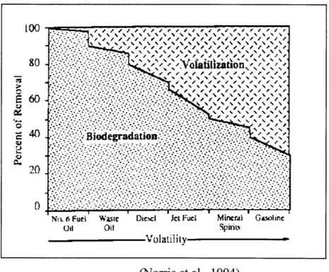
Fuel itself is composed of many different compounds. The volatility, or tendency to enter the vapor phase, of these compounds varies significantly in some instances. Many of the compounds in fuel are highly volatile. These compounds are quickly removed by stripping. However, other less volatile compounds take longer to be removed. The removal of these less volatile compounds can be expedited by

biodegradation. Figure 2-1 shows the how the primary removal mechanism will change according to the volatility of the contamination.

(Norris et al., 1994)

Figure 2-1: Volatility of different petroleum products.

2.2.2. 1. Volatilization: Free Product Removal

Free product refers to contamination that has not mixed with groundwater. In the case of a fuel spill, the fuel that remains floating atop the water table would be referred to as free product. The fuel will volatilize at a rate commensurate with its vapor pressure (VP). Vapor pressure is a measure of the tendency of a pure compound to enter the vapor phase. Vapor pressure refers to the pressure exerted by the vapor of a compound in

LVU 9o E 60. 40 20 20

No. 6 Fuel WaiW UDic Jet F-uel Mlncrdl Gisoallnc

oll Oil SpinLN

Volatilitv 01/ sF , #p 6L F- 7 -- 6 I:. · · · . .. · . · · r •a. • Fut W•slC Dt~l Jet ue.I Minral ~ a.•l·n

equilibrium with its pure liquid or solid form. Vapor pressure is a function of temperature and can be calculated from the following equation:

VP(T) = A .e(T) (2-1)

where T is temperature and A and B are constants unique to each compound.

As fuel at the source volatilizes, it is extracted by the soil vapor extraction system. The removal of this vapor phase fuel induces more of the liquid fuel to volatilize. This phenomenon occurs due to the fact that any liquid/vapor or solid/vapor system will tend towards equilibrium. Therefore, as vapor phase fuel is removed by the SVE system and "clean" air replaces the contaminated air, liquid fuel will volatilize as the system tends towards equilibrium. In reality, equilibrium is not reached, but the tendency towards equilibrium of the liquid/vapor system serves as a driving force for the volatilization and ultimate removal of fuel at the source.

2.2.2.2. Groundwater Stripping: Dissolved Contamination Removal

Some of the free product will dissolve in groundwater. Only a relatively small amount of fuel, which is made up of many different hydrocarbon compounds, will dissolve in groundwater. Most hydrocarbons are not very polar, and therefore tend to be immiscible in water, which is slightly polar. The maximum amount of any one

compound that can be dissolved in water is dictated by the aqueous solubility of that compound. Aqueous solubility refers to the amount of a compound that is dissolved in water when water is in equilibrium with an excess of that compound. Aqueous solubility

is determined empirically and aqueous solubility data can be found in reference manuals. Estimates can be made for compounds whose solubility has not been measured by using a

solubility for compounds of similar molecular size and structure.

As injected air rises in the saturated zone, it strips some of the dissolved VOCs. The amount of a dissolved compound that enters the vapor phase depends on the aqueous concentration of that compound and its Henry's law (partition) constant (H). A Henry's law constant is a measure of how a given compound will partition between water and air at equilibrium. It relates the partial pressure (Pi) exerted by a compound to its aqueous concentration (Cw) in solution:

PJ = C, -H _(2-2)

The Henry's law constant can be reported in dimensionless form or in dimensions of pressure divided by concentration (e.g. atm/(moles/L) ).

It is generally assumed that the rate at which a contaminant is removed depends on the rate at which the contaminant can diffuse through water. Such a system is said to be diffusive-flux-limited. In a diffusive-flux-limited system, the rate at which a dissolved contaminant is removed depends on the contaminant's aqueous diffusion coefficient, D, the distance that a contaminant must diffuse, L, and the concentration gradient between the contaminated groundwater and rising air:

C - Ca

J=D DC a (2-3)

L

where J is the mass flux of contaminant from groundwater to air, C, is the contaminant concentration in the groundwater and Ca is the contaminant concentration in the rising air. For modeling purposes, Ca is often assumed to be zero.

The diffusive distance, L, will vary depending on the type of air flow (bubble flow or channel flow) and will also depend on subsurface characteristics such as permeability and the degree homogeneity of the soil matrix. The diffusive distance will be a limiting factor in the removal of contamination.

Dissolved fuel may adsorb to solid particles. As groundwater flows through the soil matrix, the dissolved fuel, which is organic, is "attracted" to the organic carbon in the soil and may adhere to soil grains in a process called adsorption. This adsorbed fuel may later desorb into the liquid or vapor phase.

2.2.3. Biodegradation

Fuel is composed of hydrocarbons which are a source of energy for bacteria. In order to metabolize these hydrocarbons aerobically, bacteria need oxygen (02). However, the rate of oxygen supply below the water table is limited by diffusion and by the rate at which dissolved oxygen is consumed by microorganisms near the surface of the water

The availability of oxygen to aerobic bacteria can be greatly increased by

pumping air (and therefore oxygen) below the water table as compared to other methods of oxygen delivery. Table 2-1 shows equivalent masses of aerated water, hydrogen peroxide (H202), nitrate and sparged air required to deliver one kilogram of oxygen (02)

to the saturated zone. The increased availability of oxygen in the saturated zone enables dissolved fuel that would otherwise not have been degraded to be consumed by aerobic bacteria. The product of this degradation is carbon dioxide (CO2) and water (H20). As

with stripping, diffusion of 02 between air channels is the limiting factor in remediation time.

Table 2-1: Oxygen Availability

kg Carrier / L Carrier / Carrier kg 02 1,000 kg 02 Equivalent Equivalent Aerated Water 100,000 1 x 108 H202 (1,000 mg/L) 2,200 2 x 106 Nitrate (10g/L) 176 176,400 Air Sparging (20% 02) 4.5 55,000 (Brown et al.) 2.3. Air Channeling

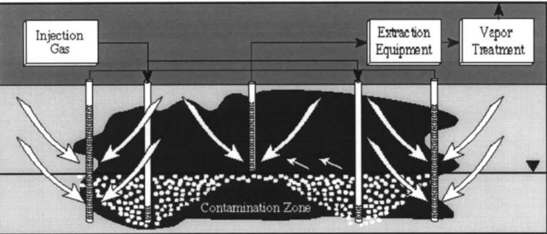
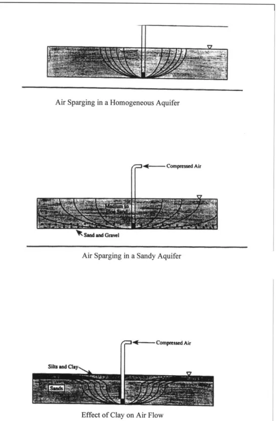
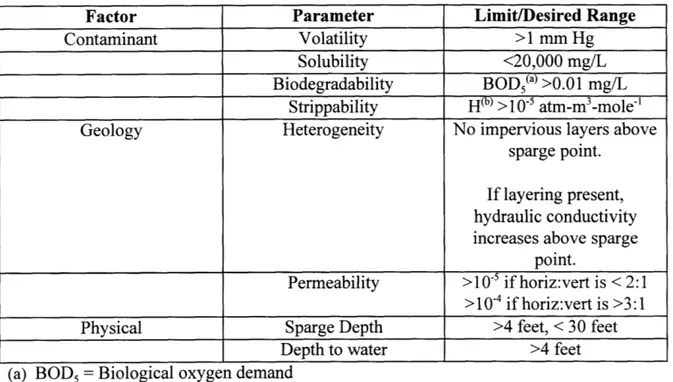
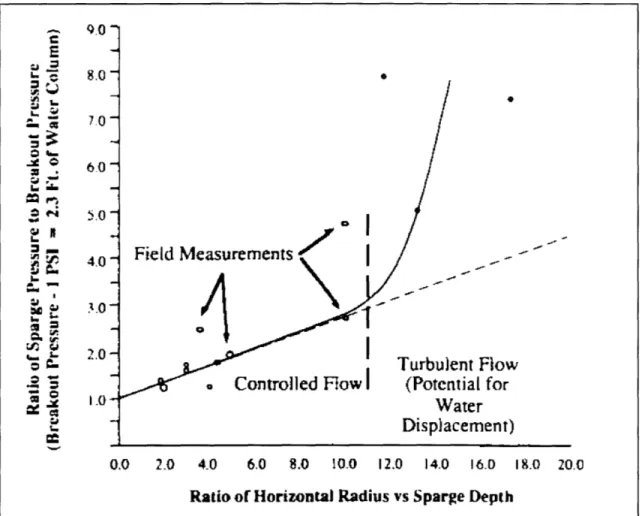
There is controversy as to whether injected air rises as discrete bubbles or forms air channels (see Figure 2-2). Most of the literature suggests that channels are formed: "Lesson, Hinchee and Vogel carried out afield study of sparging in sand in shallow standing water, and demonstrated unequivocally that channeling was the mechanism by which the injected air migrated to the top of this quite porous homogeneous medium. These results invalidate any modeling approach which does not explicitly include the effects of channeling and the associated diffusion/dispersion mass transport of both volatile/biodegradable organics and oxygen." (Wilson, Norris, and Clarke, 1996)

In a homogeneous aquifer with high permeability, the maximum distance between channels will be only several times greater than a soil pore, on the order of a few

millimeters (Norris et al., 1994). However, any zones of low permeability such as a layer of clay, skew the distribution of the air channels (see Figure 2-3). The air will flow preferentially in areas where the permeability is higher, and contamination above low permeability zones will not benefit from sparging. For sites with a high ratio of

horizontal to vertical permeability (>3:1), the general permeability of the soil matrix must be relatively high (>10'4 _{cm/s) for air sparging to be effective. (Norris et al., 1994) If the}

ratio of horizontal to vertical permeability is low (<2:1), then the general permeability of the soil matrix need not be as high (>10'5 _{cm/s) for air sparging to be effective (Norris et}

al., 1994).

The location and configuration of these channels depends on the heterogeneity and permeability of the soil matrix. A heterogeneous soil matrix will lead to preferential flow through areas of higher permeability. Therefore, removal of fuel trapped in

groundwater in between the air channels would be limited by groundwater flow. This is undesirable since it would increase total remediation time. Thus a homogeneous soil matrix is preferred to a heterogeneous matrix when air sparging is used as a remediation technology.

2.4.

Physical Site Constraints

If air sparging is to be used in conjunction with soil vapor extraction, there must be at least four feet of vadose zone. This is the minimum depth at which an SVE system can be installed. (Norris et al., 1994)

In order for air to "cone-out" from the sparge point, a minimum saturated thickness of four feet is required. Below a depth of 30 feet in the saturated zone,

prediction and control of air flow becomes difficult, and the probability of the presence of low-permeability layers increases. Table 2-2 summarizes important factors and limits in the use of air sparging. (Norris et al., 1994)

Bubble Flow (http://www.terravac.com/toolas/index/html) air compne" "--Ik m water table zone containing channels of air moving upward through the sat'd. zone

bottom of aquifer, or lower boundary of contamination

Channel Flow (Jones, 1996; Pankhow et al., 1993)

Figure 2-2: Bubble Flow vs. Channel Flow

¶z7

Air Sparging in a Homogeneous Aquifer

---

SSadandO Gravel

Air Sparging in a Sandy Aquifer

[F

gCompnased Air

-Ws .and Clay"

Effect of Clay on Air Flow

Figure 2-3: Channeled flow in the subsurface. (Jones 1996; Johnson, 1994)

--2.5.

Control of Flow

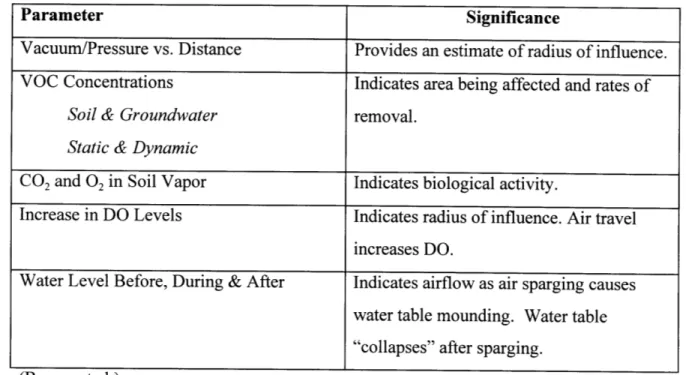
The flow of air in the saturated zone is dependent on the air injection pressure. About one pound per square inch of pressure is required to overcome every 2.3 feet of hydraulic head. At pressures slightly above the breakout pressure (the minimum pressure required to overcome the hydraulic head), the ratio of horizontal to vertical air travel is

1:2. This ratio increases as the sparge pressure increases. However, there is an injection pressure limit above which an increase in pressure will cause air flow to become turbulent (see Figure 2-4), thus wasting the extra energy input. Furthermore, dissolved

contaminants are forced away from the sparge well spreading contamination. (Norris et al., 1994)

Another concern is the water table mounding that occurs in response to air

sparging. Usually mounding induces groundwater flow away from the mound. However, the mounding induced by air sparging is caused by the physical displacement of water by air which decreases the net density of the water. This decrease in the net density of the water column counteracts the increase in the water table, preventing the water from flowing away from the mound. (Norris et al., 1994)

2.6. Radius of Influence (ROI)

In order to ensure that the full extent of the contaminated area is being exposed to sparged air, the radius of influence of the AS system must be determined. Ahlfeld et al. (1994) define the radius of influence as "the average of the furthest distance traveled by the air channels from the sparge point". There are three effective methods for

determining the ROI: measuring gas pressure in the saturated zone, measuring dissolved oxygen, and measuring increases in VOC concentration in the vadose zone. McCray et al. (1996) contend that measuring gas pressure response below the water table is the most effective way of determining the ROI.

Table 2-2: Limits To The Use Of Air Sparging

Factor Parameter Limit/Desired Range

Contaminant Volatility >1 mm Hg

Solubility <20,000 mg/L

Biodegradability BOD5(a) >0.01 mg/L

Strippability H(b) > 10- atm 3-mole-'

Geology Heterogeneity No impervious layers above

sparge point. If layering present, hydraulic conductivity increases above sparge

point.

Permeability >10-5 _{if horiz:vert is < 2:1} >10-4 if horiz:vert is >3:1 Physical Sparge Depth >4 feet, < 30 feet

Depth to water >4 feet

(a) BOD5 = Biological oxygen demand

(b) H = Henry's law constant

C E 8.0 60 I-4.0 I - _3.0 r 20 ent Flow

atial for

Ratio of Horizontal Radius vs Sparge Depth

(Norris et al.,1994)

Figure 2-4: Effect of injection pressure on air flow. __

2.7.

Pilot Studies

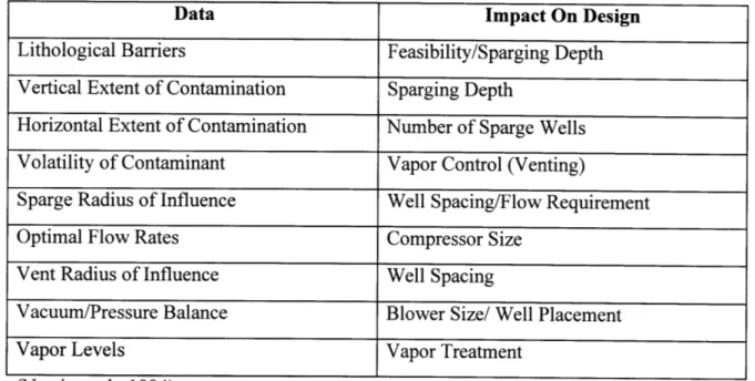
Pilot studies provide necessary empirical information that is site specific. This information is used in the design of an SVE/AS system. Table 2-3 and Table 2-4 summarize the pilot test parameters that should be monitored and provide a brief description of both the significance of the data and its impact on the design of an air sparging system.

Several parameters are of interest in a pilot study. The relationship between vacuum/pressure and distance can help determine the radius of influence. VOC concentrations are a measure of how much of the contamination is being removed. Dissolved oxygen measurements can indicate the radius of influence and the distribution of air in the subsurface. CO2 and 02 measurements can be used to test for biological

activity since microorganisms will use 02 to break down hydrocarbons and produce CO2.

Finally, water levels can reflect mounding due to air sparging. (Norris et al., 1994).

Table 2-3: Pilot Test Parameters

Parameter Significance

Vacuum/Pressure vs. Distance _{Provides an estimate of radius of influence.} VOC Concentrations _{Indicates area being affected and rates of}

Soil & Groundwater removal.

Static & Dynamic

CO2 and 02 in Soil Vapor Indicates biological activity.

Increase in DO Levels _{Indicates radius of influence. Air travel} increases DO.

Water Level Before, During & After _{Indicates airflow as air sparging causes} water table mounding. Water table "collapses" after sparging.

Table 2-4: Site And Pilot Test Data Needed For Design.

Data Impact On Design

Lithological Barriers Feasibility/Sparging Depth Vertical Extent of Contamination Sparging Depth

Horizontal Extent of Contamination Number of Sparge Wells Volatility of Contaminant Vapor Control (Venting)

Sparge Radius of Influence Well Spacing/Flow Requirement

Optimal Flow Rates Compressor Size

Vent Radius of Influence Well Spacing

Vacuum/Pressure Balance Blower Size/ Well Placement

Vapor Levels Vapor Treatment

3.

_{Modeling Air Sparging at FS-12}

3.1. Introduction

This chapter begins by describing the design of the air sparging system in operation at the FS-12. Section 3.3 describes the development of a bubble flow model used to estimate remediation time, provides a critical review of this model, and modifies the model to based on the critical analysis. Section 3.4 describes necessary modifications that must be made to the bubble flow model to account for channel flow.

3.2. Design Based on Pilot Study, HyperVentilate Model

Atlantic Sciences, Inc. designed the soil vapor extraction system and air sparging system based on the results of a model and of a pilot study. In the pilot study, the change in water pressure at different distances from the vacuum point was measured to determine the radius of influence of an SVE well. In order to determine the radius of influence of an air sparging well, several parameters were measured in the pilot study: water levels, monitoring of a tracer gas, oxygen and carbon dioxide levels in the vadose zone, air pressure and dissolved oxygen measurements.

The air permeability of the vadose zone at the FS-12 site was estimated from the results of a HyperVentilate model and from air pressure measurements conducted during the pilot study. The air permeability was estimated to lie between a range of 142-584 Darcy and an average of 305 _{Darcy. A more conservative range of 270-305 Darcy was} used as an input to the HyperVentilate program which was used to estimate the number of SVE wells required to meet remediation goals. The model yielded two results: (1) a need for a minimum of 10.6 wells based on area; and (2) a need for 30.1-34.3 wells based on critical volume. In the final design, it was decided that 21 SVE wells would suffice. The SVE system flow rate has ranged from 50 to 3500 standard cubic feet per minute (scfm). These wells have been operating at the source of the FS-12 plume since October 23,

The radius of influence of each SVE well was determined from a semi-log plot of pressure change (in. of H20) versus distance from vacuum well (ft.) from the pilot study

(see Figure 3-1). The plot was extrapolated out to a pressure change of 0.1 inches, which corresponds to a radius of influence of 160 feet. In order to be conservative, it was assumed that the SVE radius of influence was only 120 feet to ensure that all of the vapor was captured.

The radius of influence of the air sparging wells was determined from the

following parameters: water levels, a tracer gas, oxygen levels in the vadose zone, carbon dioxide levels in the vadose zone, air pressure, and dissolved oxygen (see Table 3-1).

Table 3-1: Measured Radius Of Influence

Parameter Radius of Influence (feet)

Water Levels 144

Tracer Gas 87

Oxygen Levels In Vadose Zone 87

Carbon Dioxide Levels In Vadose Zone 87

Air Pressure 87

Dissolved Oxygen 87

(Final Design Package for the FS-12 Product Recovery System, Volume II)

An effective radius of influence of 75 feet was used in the system design. The final design yielded 22 air sparging wells placed at an average of 60 feet below the water table. These wells began operation on February 21, 1996. Please refer to Figure 3-2 for a layout of the AS wells and to Figure 3-3 for a layout of the SVE.

The air sparging system is set up with "legs" extending about 60 feet below the water table. Each "leg" has two to five air sparging wells. The wells alternate in

operation in two hour cycles, with only one well operating at a time. In order for the air to reach contamination trapped in the interstitial pores spaces of the soil matrix, the

injection point is capped with a microporous tube, causing air to be released as minute bubbles and increasing the surface area per unit volume of air injected. The air injection

pressure is 30 to 40 pounds per square inch (psi). The desired flow rate is 100 scfm per AS well.

Table 3-2: Summary of key data for air sparging.

Parameter Data

Volume of fuel spill - 70,000 gallons

Plume length - 4,800 feet

Plume width - 2,750 feet

Plume vertical thickness 60-130 feet Air permeability in vadose zone 142-584 Darcy

Number of SVE wells 21

Number of AS wells 22

SVE radius of influence per well (design) 120 feet AS radius of influence per well (design) 75 feet

SVE flow rate 50-3500 scfm

C)3

LO

CD o

dL

LL

(Atlantic Sciences, Inc., 1994)

Figure 3-1: Radius of influence of soil vapor extraction wells.

E

E

aunssa-,,-(Advanced Sciences, Inc, 1994)

Figure 3-2: Layout of air sparging wells showing radii of influence

27

O PH S~'~C;~G r~LL L~~1!I~1·l ~~~!

C S~I: ~~471N~ ~5ELI~ LOI~TI~XV :;11 NR SP~li~~hi3 T)IPC

~I·1 ~NhNG SLIPE

~GLL~- lh~ FLe~

/

//

Sv 1

C) AIR; S~ARGIBs: WLLL SJCA1ION (2i~ * SCI: \AEN7IINI3 WEL LOCA II)N (21)

--- AIY b~HAMGWG PIPE

SOIL VENT NC: PI~ 61) 120

(Atlantic Sciences, Inc., 1994)

3.3. A Critical Review of an Air Sparging Model

No standard model exists for estimating the rate of removal of contamination from groundwater or the total amount of time necessary to meet remediation goals due to air sparging. However, several models have been developed that may prove to be useful in providing rough estimates and aiding in a preliminary design of an air sparging system. One such model was developed by Katherine L. Sellers and Robert P. Schreiber of Camp Dresser & McKee, Inc. (Sellers and Schreiber, 1992). In the following section, this model is described, and the assumptions behind the model development are discussed. Suggestions are made on how the model can be modified to make it more accurate when applied to FS-12. Specifically, diffusion coefficients for major components of JP-4 jet fuel are calculated and incorporated into a decay coefficient. This decay coefficient is used to create plots of exponential decay of concentration versus time for the major components of JP-4 jet fuel. Finally, the time required for benzene, toluene,

ethylbenzene, and xylene to reach their maximum contaminant levels (MCL) of 5 part per billion (ppb) is estimated.

Air Sparging Model for Predicting Groundwater Cleanup Rate

by: Katherine L. Sellers and Robert P. Schreiber, Camp Dresser & McKee, Inc.

3.3.1. Assumptions of Sellers and Schreiber Model

Air Flow in the Saturated Zone

* Air rises as discrete spherical bubbles.

* A low flow rate is assumed when calculating an effective bubble radius. * There is an even distribution of sparged air bubbles in volume of influence.

(Volume of influence is defined as the volume of groundwater within the radius of influence of an individual air sparger.)

* The distance that a bubble travels is taken to be the average depth of the sparge points below the water table.

Subsurface Characteristics

* There is high uniform porosity and permeability as typically found in sand or gravel (low sorption capacity).

* The soil matrix is homogeneous and isotropic. * Subsurface air temperature is 100_C.

Spargers

* Radii of influence of individual spargers do not overlap. Rate of Contamination Removal

* Remediation time and rate of contamination removal are dependent on contamination volatilization rate only. (No biodegradation of contaminants occurs.)

* The diffusive distance is equal to the bubble radius.

* Equilibrium is not reached. Therefore, the contamination removal rate is diffusive-flux-limited.

Mixing

* The groundwater in the sparged zone is well mixed. Other

* The model does not account for free product removal.

* The bubble terminal rise velocity approximation assumes that the bubble is rising in water only.

3.3.2. Measured Parameters

C(t) = _{average concentration of groundwater contamination in sparged plume;}

Q

d = _{fraction of 24-hour day that the air sparging system is in operation;} h = depth of screen below groundwater table;

R = radius of sparger openings;

Roi = radius of influence of individual sparger; n = average porosity of soil

3.3.3. Estimated Parameters

D = _{diffusion coefficient of contaminant in water: 9 x 10}

-6 to 1.09 x 10-5 cm2/S

(Hayduk and Laudie, 1974);

L = _{distance over which contamination must diffuse; assumed to be equal to average} effective radius, r, of a sparged bubble;

rb = average effective radius of sparged bubble; for low flow conditions of air

injection into water, r can be approximated by:

rb = 2-R 2 a, Y)g] (Orr, 1966) (3-1)

R

(p

water

air

R = radius of sparger openings

a = air-water surface tension (0.0728 N/m) pwater= density of water (1,000 kg/m3₎

pair = density of air (1.29 kg/m3 at 100C)

g = gravitational constant (9.81 m/s2₎ rb is typically 0.5 to 2 mm.

Sb/Vb= average surface area to volume ratio of a bubble;

4xr 2 ₃

Sb/ Vb= 43r -i (3-2)

(4/3) 7rr, rb

Vb = terminal velocity of rising bubble

F

Vh = 1.04g rb + p

j7

g = gravitational constant (9.81 m/s2₎ rb = bubble radius

c = air-water surface tension (0.0728 N/m)

pwater = density of water (1,000 kg/m3₎

Vs = volume of water in the contaminant plume that is in contact with sparging

bubbles; equal to the sum of the volume of influence of individual spargers;

V = RR -h-n (see Figure 3-4)

Vi = volume of influence of an individual sparger;

Roi= radius of influence of individual sparger; h = depth of sparge point below the water table; n = porosity;

Vs = k.rRo2, -h-n

k = number of spargers

(Sellers and Schreiber, 1992)

Figure 3-4: Volume of influence.

(3-4)

(3-5)

f

individual spargers to the plume area (see Figure 3-5): I

_Ai

f = 0 Acont

n = number of air spargers; Acont = total area of contamination;

Ai = area of influence of an individual sparger; A, = 7r Ro2i

Roi = radius of influence of individual sparger

(3-6)

(3-7)

3.3.4. Description of Model

The mass transfer of contamination from groundwater to air can be modeled by Fickian diffusion:

Jt = [C(t)

J(t) = D

_(3-8)

J(t)= mass flux density of contamination from groundwater to air; dimension of mass flux density = mass

(unit area)(time)

D = diffusion coefficient of contamination in water,

l12

Pq a rF ll I1 ,lr ILEI I I rl Jir L Ul::NY _ CONTAI S GROUND' FLO' DIREC1

(Sellers and Schreiber, 1992)

Figure 3-5: Area of influence,f.

Area of plume contamination and radii of influence of air sparging wells. The variable

fis

equal to the sum of the area of influence of all of the individual air sparging wells divided b Ai

by the plume area, f 0

L _{= distance over which contamination must diffuse; assumed to be equal to} average effective radius, r, of a sparged bubble (see Figure 3-6);

(Sellers and Schreiber, 1992)

Figure 3-6: Diffusive distance in bubble flow.

The diffusive distance is assumed to be equal to the bubble radius.

The contaminant concentration of a bubble that has reached the water table,

Cair(t), is equal to the mass flux density multiplied by the surface area to volume ratio of a bubble multiplied by the time it takes the bubble to travel from the sparge point to the groundwater surface.

Cir (t) = J(t) (Sb/Vb) -T (3-9)

Cair(t) = _{contaminant concentration in bubble upon reaching the water table;}

Sb/Vb = average surface area to volume ratio of a bubble;

T _{= time for bubble to travel from injection point to water table;}

The time it takes for a bubble to reach the groundwater surface is estimated by taking the depth of the injection point below the water table and dividing it by the bubble terminal rise velocity.

L = DIFFUSIVE DISTANCE _{AIR BUBBLE}

h

T =- (3-10)

h = average depth of sparge points below water table;

Vb = terminal rise velocity of bubble;

Eq. 3-9 is can be derived from a simple mass balance; the mass of contamination

contained in a bubble, M, which has reached the groundwater surface is equal to the concentration of contamination in the bubble, Cair(t), multiplied by the volume of the bubble, Vb:

M = Cair(t) Vb _(3-11)

Likewise, the total mass of contamination transferred from groundwater to a bubble, M, is equal to the mass flux density of contamination to the bubble, J(t), multiplied by the surface area of the bubble, Sb, multiplied by the residence time of the bubble in groundwater, T:

M = J(t) -Sb T _(3-12)

Setting Eq. 3-11 equal to Eq. 3-12, yields:

Ca,, (t). Vb = J(t) Sb

-

Solving for Cair(t) yields Eq. 3-9:

Car (t)= J(t). (Sb/Vb)

T

Substitution of Eq. 3-8 and Eq. 3-10 into Eq. 3-9 yields:

Cair D. C(t)

-(Sh/Vb)'

dM

The rate of removal of contaminant mass, d, from the groundwater to the injected air can estimated by multiplying the concentration of contamination in air, Cair(t),

by the air flow rate in the saturated zone,

Q:

In order to more accurately describe the rate of mass removal, Eq. 3-15 can be modified to account for the actual fraction of the plume that is sparged,

f(see

dM

dt - -

f

Q

The contaminant mass removal rate can also be defined by the change in concentration of contamination in the groundwater per unit time,

groundwater affected by air sparging, Vs:

dM dC(t) dt -Vdt

dt dt

Equating Eq. 3-16 and Eq. 3-17, and then solving for

dC(t) Q

dtS t - - f -d -Ca,

(t)

-Substitution of Eq. 3-14 into Eq. 3-18 yields:

dC(t)

dt•, multiplied by the volume of

_dt

(3-17) dC(t) dt, yields:

dt

dC(t)

Defining the constant B as:

B

=f

-

d

-

(Sb/V,)

(

_R

h

and substituting B into Eq. 3-19 yields: dC(t)

dC) =

-B -C(t)

-

fd

-

(Sh/V,)

L (h

-C(t)

Solving this differential equation explicitly for C(t) yields an exponential equation:

C(t) = Co e-B- _(3-22)

C_o = initial concentration of contaminant in groundwater; C(t) = contaminant concentration in groundwater at time t;

3.3.5. Model Analysis Well-Mixed Assumption

The model assumes that the groundwater affected by the sparged bubbles is well-mixed with the unaffected groundwater. The concentration C(t) used in the model represents an average concentration of contamination in the plume. (Sellers and Schreiber, 1992)

Within the sparged zone, groundwater mixes via two mechanisms: (1) local convective movement around the sparger ; and (2) the displacement of water by the rising air bubbles. Pulsed air injection, which refers to the periodic shut down and restart of the injection system, can enhance mixing. When air injection ceases, groundwater will replace the volume previously occupied by the sparged air. This process enhances mixing of sparged and unsparged groundwater. In short, the well-mixed assumption provides a good approximation of conditions in the sparged zone. (Sellers and Schreiber,

1992)

No Biodegradation

The model does not account for the biodegradation of contaminants. This leads to an overestimation of remediation time at the FS-12 site, since JP-4 jet fuel contains biodegradable contaminants. Thus, despite the fact that neglecting biodegradation renders the model less accurate when applied to FS-12, at least the model errs on the conservative side.

Bubble Travel Time

The time it takes for an injected bubble to rise to the groundwater surface is estimated by taking the depth below the water table, and dividing it by the terminal rise velocity, Vb.

h

T - (3-10)

Implicit in this estimation is the straight path of a bubble from the sparge point to the groundwater surface. However, the true path of a bubble is tortuous as it weaves in between soil grains. Therefore, the bubble travels a longer distance than just the depth, h, from the water table to the sparge point. A longer distance traveled will lead to a longer travel time, T, _{which will lead to an increase in mass flux. This increase in mass flux,}

reflected in the increase of the constant B, will lead to a higher contamination removal rate:

B

=f

-

d

-

-

)

_(3-20)

C(t) = Co e -B _(3-22)

Futhermore, the approximation (Eq. 3-3) for the bubble terminal rise velocity, v, is valid for a bubble rising in water only. The presence of soil grains will lead to a decrease in the terminal rise velocity found from Eq. 3-3. Therefore, a bubble terminal rise velocity computed from Eq. 3-3 will overestimate the true bubble terminal rise velocity. This overestimation of the bubble terminal rise velocity will cause the bubble residence time, T, _{to be underestimated which will lead to an underestimation of the}

contamination removal rate.

In order to more accurately estimate the contamination removal rate, a factor for tortuosity, -, _{can be included in the model:}

r T, (1.34 Lecture Notes 2, 1997) _(3-23)

1 = macroscopic straightline distance between two points

l_e = effective transport distance between two points Eq. 3-23 can be solved for le:

le- _(3-24)

In applying Eq. 3-24 into the air sparging model, the macroscopic straightline distance, 1, is equal to the sparger depth, h, below the water table:

h

The effective transport distance, le, _{is a more accurate representation of the actual}

distance that a rising bubble travels than the sparger depth, h. Substituting le from Eq. 3-23 for h in Eq. 3-10, yields a more accurate bubble residence time:

l h

T l - _(3-26)

Vb Vhb4

Substituting Eq. 3-24 into Eq. 3-20 yields:

B =

f

-d -

Flow Rate and Injection Depth

The model was able to successfully approximate contamination removal rate in two case studies. (Sellers and Schreiber, 1992) However, in those case studies, the air flow rates ranged only from 2 to 11 cfm. At FS-12, the estimated flow rate is 100 cfm. Furthermore, in one of the cases, the maximum depth of air injection was 11 feet. At

FS-12, the air is injected at an average of 60 feet below the water table. These differences may be significant when attempting apply the model to FS-12.

Estimation ofDiffusivities

The contamination at FS-12 is JP-4 jet fuel is composed of many different components (see Table 3-3). The model assumes that all the components of the JP-4 jet fuel have the same aqueous diffusivities, 10-' m2_{/s. In reality, each component diffuses at}

a different rate. The diffusion coefficients for each of the components can be estimated as a function of its molar volume and the viscosity of water:

13.26 x 10-5

D, = (cm2_s-1_{) (Hayduk and Laudie, 1974)}

(3-28)

P. /14 .V 0.589

C, = viscosity of water in centipoise (10-2g cm's-1)

V = molar volume of chemical

Table 3-3 shows a break down of the 28 major components in JP-4 jet fuel and shows the concentration of each of these components in the fuel. Table 3-4 shows the

Table 3-3: Break Down of Major Components of JP-4 jet fuel Component Concentration (g/L) n-butane 4.92 iso-pentane 2.6 n-pentane 2.07 2-methylpentane 7.43 3-methylpentane 6.48 n-hexane _17.9 methylcyclopentane 11.6 benzene _7.82 cyclohexane 9.63 2-methylhexane 28 3-methylhexane 27.1 dimethylhexane 6.21 n-heptane 33.1 methylcyclohexane 22 toluene 10.7 2-methylheptane 16.5 3-methlyheptane 12.4 n-octane 21.3 ethylbenzene 9.89 m- and p-xylene 12.5 o-xylene 2.04 n-nonane 1.54 n-decane _5.22 n-undecane _2.68 napthalene ND* n-dodecane ND n-tridecane ND n-tetradeane ND

Table 3-4: Molecular Weight, Density, Diffusion Coefficients, and Decay Coefficients of BTEX

Component Molecular Density (mg/L) Diffusion (cm2_{/s) Decay}

Weight (g/mol) at 20 OC Coefficient Coefficient (day-1₎

benzene 78.2 0.8765 9.41 E-06 8.6E-04

toluene 92.1 0.8669 8.49E-06 7.8E-04

ethylbenzene 106.2 0.867 7.81E-06 7.1E-04

xylenes 106.2 0.8611 7.78E-06 7.1E-04

molecular weight of benzene, toluene, ethylbenzene, and xylene (BTEX), the density of each BTEX component at 200_{C, the aqueous diffusion coefficient of each BTEX}

component, and their corresponding decay coefficients.

The decay coefficients were calculated from input parameters, which included both measured parameters and estimated parameters (see Table 3-5 and Table 3-6).

B =f -d -(Sb/Vb) 7 h (3-20)

Table 3-5: Measured Parameters for Bubble Flow Model

Symbol Name Value

Q total air flow rate _{2,100 cfm (85,300 m}3_/d) d fraction of day that AS system is in operation 0.25

h depth of sparge point below water table 60 ft (18.3 m)

R radius of sparger opening _{0.01 in (0.000254 m)}

Ro, _{radius of influence of individual sparger 75 ft (23 m)}

n porosity _0.35

Table 3-6: Estimated Parameters for Bubble Flow Model

Symbol Name Value

r bubble radius 0.0045 m

SN bubble surface area to volume ratio 670 m-1

v bubble terminal rise velocity 0.25 m/s

V, volume of influence 220,000 m3

f _{fraction of contaminant plume sparged 0.73}

The time to reach MCLs was calculated for benzene, toluene, ethylbenzene, and xylene (BTEX). It was found that benzene and toluene required the most time to reach

MCLs. Concentration profiles of benzene and toluene under both the bubble flow and channel flow models were developed and compared (see Chapter 4). Detailed results of calculations can be found in the Appendix.

3.4. Air Channeling Applied to Model

A fundamental assumption in the Sellers and Schreiber model is that injected air rises as discrete bubbles. Most of the literature on air sparging suggests that air rises in channels. The model can be changed to describe the groundwater cleanup rate for air rising in channels.

Changes must be made in three aspects of the above model to account for air channeling: (1) the surface area to volume ratio, (2) the diffusive distance, (3) the air rise velocity.

Surface Area to Volume Ratio

The surface area over which mass flux of contamination occurs changes when air flow is modeled as channels instead of discrete bubbles. Air channels can be

approximated as cylinders, and the surface area to volume ratio of a cylinder can be derived as follows:

Sc = 2rrc h (3-29)

Sc = surface area of an air channel; rc = radius of air channel;

h = depth from groundwater surface sparge point;

Vc = 7rc h (3-30)

Vc = volume of an air channel 2:rrc h 2

Sc/

V

r-Diffusive Distance

When air flow is modeled as channels, the maximum diffusive distance becomes half of the distance between air channels, s/2. The distance between air channels is only several times the pores size (Norris et al., 1994). For the purposes of this model, a

distance of 9 mm will be assumed to be the distance between air channels. Eq. 3-8 can be modified to reflect this change by substituting L with s/2:

J(t) = DC(t) (3-8)

Substituting L with s/2, yields:

J(t)=

D •c(t

2D-

j

(3-32)

Air Rise Velocity

The velocity by which injected air rises is channel flow can be found from the total volumetric flow rate, Q, and the total cross-sectional area of the channels, Ax, . The total area through the air channels, Ax, , through which the air passes will be determined by the radius of the air channels, rc, and the number of air channels, N. The terminal rise velocity, vc, of the injected air can then be expressed as follows:

Q (3-33)

Q = total volumetric air flow rate

AxT = total channel area (through which injected air passes)

Ax, = N Axch (3-34)

N = number of air channels

Axc = cross-sectional area of individual air channel

The number of channels, N, can be estimated by first estimating a channel density. It is assumed that there is one channel per area defined by the following equation (see Figure 3-8):

Arc+ = (2rc + s)2 (3-36)

rc = channel radius s = diffusive distance

The number of channels, N, can be estimated by taking the total area of contamination, Acont and dividing by Arc+:

Acont N-A r +s

7

Ax, = cross-sectional area of channel s = distance between channels rc = channel radius

Figure 3-7: Channel cross-sectional area and diffusive distance between channels.

Figure 3-8: Area used to estimate channel density.

As in the bubble flow model, the channel flow model is based on a lumped

parameter decay coefficient, B. Incorporating the changes described above into B, yields:

B=

f

-d -

(Sc/VC)

h&

_(3-38)

Table 3-7, Table 3-8, and Table 3-9 show the input parameters to calculate the decay coefficients found in Table 3-9 for channel flow.

Table 3-7: Measured Parameters for Channel Flow Model.

Symbol Name Value

Q total air flow rate 2,100 cfm (85,300 m3/d)

d fraction of day that AS system is in operation 0.25

h _{depth of sparge point below water table 60 ft (18.3 m)} R radius of sparger opening 0.01 in (0.000254 m) Roi radius of influence of individual sparger 75 ft (23 m)

Table 3-8: Estimated Parameters for Channel Flow Model

Symbol Name Value

r channel radius 0.002 m

SN bubble surface area to volume ratio 1000 m-1 v bubble terminal rise velocity 33 m/s

V, volume of influence 220,000 m3

f fraction of contaminant plume sparged 0.73

Table 3-9: Diffusion coefficients and channel flow decay coefficients for BTEX.

Component Diffusion Decay

Coefficient (cm2/s) Coefficient (day-_')

benzene 9.41 E-06 8.1 E-06

toluene 8.49E-06 7.3E-06

ethylbenzene 7.81 E-06 6.8E-06

4.

Results and Discussion

The time for a contaminant to reach its MCL is dependent upon the lumped parameter decay coefficient, B, in both the bubble flow model and the channel flow model. Slight differences in B can lead to significant changes in concentration profiles, since concentration varies exponentially with B:

C(t) = C, e-B

(3-22)

For bubble flow:

B= f -d -(S/V,)

(

(

-

(3-20)

For channel flow:

B =f -d -(S/V)

_(3-34)

Table 4-1 compares decay coefficients for BTEX for the two models, bubble and channel flow. The large discrepancy in the values of the decay coefficients between bubble flow and channel flow are predominantly a result of the difference in the terminal rise velocities between the two models (see Table 4-2).

Table 4-1: Comparison of decay coefficients for bubble flow and channel flow.

Compound benzene toluene ethylbenzene xylene Decay Coefficients (day- )

Bubble Flow Channel Flow

8.6E-04 9.6E-06

7.8E-04 8.6E-06

7.1E-04 7.9E-06

Table 4-2: Comparison of terminal rise velocities, bubble and channel radii, and diffusive distance for bubble and channel flow.

Parameter Bubble Flow Channel Flow

Air Rise Velocities 0.25 m/s 12.6 m/s

Bubble or Channel Radius 4.5 mm 4.5 mm Diffusive Distance 4.5 mm 4.5 mm

Another parameter which will have a significant effect on the decay coefficient is the bubble or channel radius. In both models, mass transfer increases with decreasing radius, because the surface area to volume ratio, S/V, will increase as bubble or channel radius increases:

Bubble Flow Channel Flow

S 3

V rb

S 2 V rh

It is important to note that it was assumed that the channel radius was equal to the bubble radius, and that the channel radius was not calculated from an empirical equation nor derived from scientific principles. It was also assumed that the diffusive distance for channel flow, s/2, _{is equal to that for bubble flow, L. These assumptions magnify the} importance of the difference in air rise velocities between the two models.

Table 4-3: Time for BTEX components to Reach MCLs.

BTEX Benzene Toluene Ethylbenzene Xylenes

* Advanced Sciences. Inc..

Co (ppm)*

Table 4-3 compares the time required in for BTEX components to reach MCLs for both the bubble flow model and the channel flow model. Figure 4-1 and Figure 4-2

748.5 815.4 214

illustrate the significant disparity between the remediation rates if the two models. In both models, toluene took longest reach its MCL followed by benzene. The channel flow results seem to indicate that volatilization from air sparging is not an effective

remediation mechanism, however biodegradation may still be possible.

Concentration vs. Time

0.045

* * Benzene- Bubble Flow Model

0.035 Benzene - Channel Flow Model

0.03 0.025 -- 0.02-0.015 ----0.011 0.1 1 10 100 1000 Time (years)

Figure 4-1: Comparison of benzene concentration profiles for bubble flow and channel flow.

E a a c o c r a, u c o o 0.1

*Toluene - Bubble Flow Model SToluene - Channel Flow Model

10 100 1000

Time (years)

Figure 4-2: Comparison of toluene concentration profiles for bubble flow and channel flow.

The bubble flow results indicate that air sparging is a plausible remediation technology for JP-4 jet fuel, since remediation time considering only volatilization is less than 10 years.

Concentration vs. Time

---5.

Conclusions and Recommendations

Air sparging remediation time at FS-12 was estimated using two models: a bubble flow model and a channel flow model. Each model considered contamination removal by volatilization only. The bubble model yielded remediation time estimates under 10 years. If biodegradation were to be included in the bubble model, remediation time would decrease.

Channel flow results indicate that volatilization from air sparging is not a viable mechanism for contaminant removal. However, the model does not discount

biodegradation as a viable mechanism. Many of the compounds found in JP-4 jet fuel could be easily biodegraded in nutrient rich soils. The kinetics of the biodegredation of components of JP-4 jet fuel should by investigated to better assess air sparging as a remediation alternative at FS-12.

In addition to neglecting biodegradation, the post-sparging effects of dilution and dispersion were not considered. Combined with groundwater contamination removal, these would further decrease concentrations.

One scenario not considered in this report is the possibility that some air rises as discrete bubbles and some rises as channels. The potential for both types of flow to coexist should be investigated.

References

Advanced Sciences, Inc., Final Design Package for the FS-12 Product Recovery System: Design Calculations. Vol 2,3 June 1994.

Atlantic Environmental Technologies, Inc., Monthly Report, October 23 -November 22,

1995, January 23 - February 22, 1996.

Brown, R. A., Hicks, R. J., and Hicks, P. M. "Use of Air Sparging for In-Situ Bioremediation." ed. Hinchee, Robert E., CRC Press, Inc., 1994.

Culligan-Hensley, Patricia. 1.34 Lecture Notes 13, Problem Set # 3, 1997. Davis, Bob. Personal communication, January-May, 1997

http://www.afcee.brooks.af.mil/pro..main/fact/fact/sdw9 96/09 96 3.HTM http://www.aristotle.com/Sparging/TechResponses/whatis/ResponseMenu.html http://www.terravac.com/toolas/index/html

Jones, Karen. An Analysis of Air Sparging/Soil Vapor Extraction Systems Emphasizing Volatilization Kinetics in JP-4 Jet Fuel. Massachusetts Institute of Technology,

1996.

McCray, John E., Falta, Ronald W. "Defining the air sparging radius of influence for groundwater remediation." Journal of Contaminant Hydrology. Vol. 24. 1996 Norris, Robert D. et al. Handbook of Bioremediation, CRC Press, Inc., 1994.

Pankhow, James F., et al. "Air Sparging in Gate Wells in Cutoff Walls and Trenches for Control of Plumes of Volatile Organic Compounds." Groundwater. Vol. 31, No. 4, 1993

Pesce, Edward, Personal communication. January-May, 1997.

Schreiber, Robert P., Sellers, Katherine L., "Air Sparging Model for Predicting

Groundwater Cleanup Rate." Proceedings of the 1992 Petroleum Hydrocarbons and Organic Chemicals in Ground Water: Prevention, Detection, and