Analog Computer Research

Prof. E. A Guillemin N. DeClaris M. S. Macrakis

Prof. R. E. Scott Y. C. Ho T. E. Stern

A. APPLICATIONS OF SIGNAL FLOW GRAPHS TO ANALOG COMPUTERS

With the aid of various flow-graph transformations, these two goals are to be attained: (a) the construction of a flow graph representing the fundamental relations between equation variables which will be physically realizable on a computer, and

(b) the reduction of this flow graph to one that uses a minimum number of components. This latter factor is important for reasons of economy and accuracy.

1. Transformations

In implementing these goals, the concept of flow-graph transformation is a useful tool. Basic transformations which may be performed on a linear flow graph are:

cas-cade transformations, parallel transformations, replacement of a self-loop by a branch, and branch inversion. These transformations have been defined and discussed by Prof. S. J. Mason of this Laboratory (1).

Various special combinations of these basic transformations are of value in dealing with computer connection diagrams. An example is flow-graph inversion, which is

defined as any combination of transformations on a flow graph that changes the classi-fication of all terminal nodes without changing the fundamental relations between the variables. That is, all nodes which were originally sources must become either inter-mediate nodes or sinks, while all nodes which were originally sinks must become

sources.

As an illustration of the properties of the flow-graph inversion, let us write a set of simultaneous equations in the matrix form

ax= s

where the elements of a may be linear differential operators. In this form, all the unknowns are to the left of the equality sign and all of the known functions of the indepen-dent variable are to the right. If a flow graph representing these relations is drawn, all of the unknowns appear as sources and all of the knowns as sinks. Normally, solving this set involves inversion of the coefficient matrix. This inversion process is a means of expressing the unknowns as functions of the knowns. In the same way, flow-graph inversion is a means of expressing the unknown nodes in terms of the known nodes in order to solve the equations of the flow graph. There is a direct analogy between flow-graph inversion and matrix inversion.

(XVII. ANALOG COMPUTER RESEARCH)

2. Optimization Procedure

The basic steps used to proceed from a set of equations to the final connection diag-gram are: (a) Construct the flow graph from the original equations. (b) Invert the flow graph. (c) Utilize additional transformations to make the graph physically realizable on the proposed computer, to reduce the number of integrators to the theoretical minimum, and to reduce the total number of components to a minimum.

Let us assume that we have available an electronic analog computer containing only adders, integrators, phase-inverters (each of which introduces unavoidable phase inver-sion), and arbitrary function (of time) generators. As an illustration of the flow-graph procedure we shall obtain an optimum computer diagram for the following set of equations.

S+ 1 + + 2 + + 2 + x2+x 3 = Sl(t)

il + l

1+ x

3

= S

2

(t)

X2 + x2 + x3 = S

3

(t)

Although the sum of the orders of the highest derivatives of each unknown in this set is 6, the determinant of the operational coefficients, and hence the true order of the set, is 4 (see ref. 2). Thus we should be able to obtain a computer connection involving only 4 integrators.

The steps in proceeding from the original flow graph to the final computer connection are shown in Fig. XVII-1. Figure XVII-1(a) is the original graph. (S is used to repre-sent time differentiation.) The checked branches are inverted to obtain the graph of Fig. XVII-l(b). With the aid of additional transformations and the introduction of various auxiliary nodes, the final graph (Fig. XVII-I(c)) is obtained. In Fig. XVII-2, the final graph is represented in conventional computer notation and compared with another con-nection diagram derived for the same set of equations by a conventional method. Note that the conventional connection contains 2 more integrators, and a total of 3 more com-ponents than the connection derived through flow graphs.

T. E. Stern

References

1. S. J. Mason, Feedback theory - some properties of signal flow graphs, Technical Report No. 153, Research Laboratory of Electronics, M. I. T., 1953; and Proc. I.R.E. 41, 1144-1156 (Sept. 1953).

2. F. B. Hildebrand, Advanced calculus for engineers (Prentice-Hall, New York,

1950) p. 23.

-82-(XVII. ANALOG COMPUTER RESEARCH)

B. TIME-DOMAIN SYNTHESIS BY DELAY-LINE TECHNIQUES

An artificial delay line is being used to evaluate some techniques for time-domain synthesis. The first step in time-domain synthesis usually involves the determination of the impulse response h(t) of a network. Dr. M. V. Cerrillo's work on scanning func-tions (1) shows that, in general, through the solution of a particular set of simultaneous equations, it is possible to determine h(t) so that it obeys the following relation

n

G(s) = F(s) aksk = F(s) H(s) (1)

k=O

where G(s) is the Laplace transform of the output time function g(t); F(s) is the Laplace transform of the input time function f(t); and H(s) is the Laplace transform of the impulse response h(t). This relation will hold for small values of s; that is, g(t) will follow the desired response except at points of discontinuity of the input time function f(t).

Dr. Cerrillo's scanning function, upon investigation, turns out to be very similar to the transfer functions of sampled-data systems derived from a different basis (2, 3).

Certain simple examples have been checked analytically and experimentally, and found to give similar results from both methods of approach. There thus exists a distinct possibility of applying the techniques of one method to the other to faciliate the synthesis procedure. Further investigations are in progress.

Y. C. Ho

References

1. This work will be discussed in the forthcoming Technical Report No. 270 by M. V. Cerrillo.

2. J. M. Salzer, Frequency analysis of digital computers operating in real time, Proc. I.R.E. 42, 457-466 (Feb. 1954).

3. W. K. Linvill, Use of sampled functions for time domain synthesis, Proc. N. E. C. 9, 533-542 (Sept. 1953).

C. DRIVING-POINT IMPEDANCE OF RC NETWORKS TERMINATED IN AN INDUCTANCE

The importance of LC networks terminated in a 1-ohm resistance was well demon-strated by Darlington (1) in his method of driving-point impedance synthesis. This study is undertaken in an attempt to establish the effect on an RC driving-point impedance of adding a single inductance at some point in the circuit.

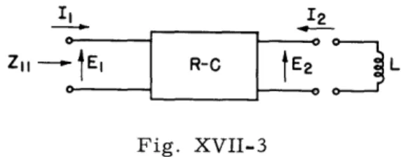
Consider an RC network terminated in an inductance L, shown in Fig. XVII-3. In general, for a two-pair terminal network we have

-84-E = Z11 1 + Z12 1Z

(1)

E₂ Z 12 _{1 + z22 2}

Since, in this case, E2 = -Ls 12, it is easy to derive

2 E_l Z₁1Z2 2 - zZ + Z Ls Z 1 z22 Ls 11 I z +Ls or 1/y2 2 + Ls

z

₁₁

= z

_{11 Z + Ls}

(3)

where z11 Y22 2 z 1 1 z 2 - z

is the short-circuited driving-point admittance of the RC network.

It is well known that for an RC network the driving-point impedance and admittance have real negative poles and zeros which alternate along the real axis of the s-plane. Therefore n? P(s) F1 (s + pi) z = - k = k (4) Q(s) (s +qi ₎ i=l

where n' = m', or n' + 1 = m', and ql < p1

.

Similarly,

D(s)

(s + d

l

)(s + d

Z ) .

..

z = k = k s (s + q2) ql < d (5) 2

Q()

2

(s

)(

+

)

<d

1

(5)

M(s) (s + ml)(s + ₂) ... (s + mm) Y2 ₂₂ = k3 _{3 N(s)} k _{3 (s + n} m < n (6) l )(s + n2). (s + n) 1 1 By substitution, Eq. 3 becomes

P(s) N(s) + c lSLM(s)

11

M(s) D(s) + c

2

sLQ(s) c

3

(7)

where 1 k1 c =k 3 c c -1 3' kZ ' 3 kk ₃

II 12

,--I

-0 t

Z11 - I El R-C E2 L

Fig. XVII-3

RC network terminated to one inductance.

Fig. XVII-4

The polynomials M(s) and N(s) for real s.

Fig.

The polynomial

XVII-5

sM(s) for real s.

-86-Let us study the polynomial

R(s) = N(s) + c lLs M(s) (8)

N(s) and M(s) have all of their roots real negative (-n i, -n Z , . . . , -nn , and -m, -m2'

... , -mm) which alternate when arranged in a sequence according to their ascending magnitude. A sketch of N(s) and M(s) is given in Fig. XVII-4 for s real and negative. Both M(s) and N(s) start positive, since M(O) = mlm2m3... mm, and N(0) = n 2n3... nn

A plot of the polynomial s M(s) is given in Fig. XVII-5. Observe that s M(s) < 0 for 0 > s > -m ' since M(s) is positive for that region and s is negative real.

According to the fundamental theorem of algebra (2), the total number of roots of the polynomial R(s) is m + 1. By inspection of Fig. XVII-5 it is obvious that regardless of the magnitude of N, M, and L there will be one, and only one, zero of R(s) in the region -n. > s > -mi+1l where i = 1, 2, ... ., m. Therefore, regardless of the value of L the

polynomial R(s) will always have m-l real and negative roots. No real roots exist in the intervals -m. > s > -n. where i = 1, 2, ... , m.

1 1

There remain two additional roots. If these roots are to be real, at least one must occur in the region

0 < s < - 1 (9)

However, by reference to Fig. XVII-5 it is possible to select a value L such that no real root of R(s) exists in the interval 0 < s < -mI. Hence, by elimination, the two remaining roots must be complex conjugates. As a result the following can be stated.

Theorem: The driving-point impedance of an RC network terminated to an inductance will have at most one pair of complex conjugate zeros and one pair of complex conjugate poles.

Corollary: The driving-point impedance of any 2-terminal linear passive RLC network may have any number of pairs of complex conjugate poles up to, and not exceeding, the total number of nonsuperfluous inductors or capacitors, whichever is the least.

A similar analysis can be carried out for an RL network terminated to a capacitor. N. DeClaris

References

1. S. J. Darlington, J. Math. Phys. XVIII-4, 280 (1939).

2. L. L. Walsh, Location of the critical points of rational functions in the complex domain, Am. Math. Soc. Colloquium Publication, Vol. 34 (1950).