Analysis of Magnetic Activity Cycles in Solar Analogs Using Solar - Stellar
Spectrograph Data
by
Duy Anh N. Doan
Submitted to the Department of Earth, Atmospheric and Planetary Sciences
in Partial Fulfillment of the Requirements for the Degree of
Bachelor of Science in Earth, Atmospheric and Planetary Sciences
at the Massachusetts Institute of Technology
June 2016
Copyright 2016 Duy Anh N. Doan. All rights reserved.
The author hereby grants to MIT permission to reproduce and to distribute publicly paper and electronic copies of this thesis document in whole or in part in any medium now known or hereafter created.
AuthorSignature
red acted
Author
Duy Anh N. Doan Department of Earth, Atmospheric and Planetary Sciences May 18, 2016
Certified b
Signature redacted
Amanda Bosh
Accepted by
Thesis Supervisor
Signature redacted
Tanja Bosak Chair, Committee on Undergraduate Program MASSACHUSETTS INSTITUTE OF TECHNOLOGY
SEP 28 2017
LIBRARIES
ARCHIVES
1MITLibraries
DISCLAIMER NOTICE
Due to the condition of the original material, there are unavoidable
flaws in this reproduction. We have made every effort possible to
provide you with the best copy available.
Thank you.
Thesis contains Table of Contents pagination
irregularities.
Table of Contents
I.
A bstract ...
3
II.
Introduction...
4
III.
A nalytical M ethods...
5
IV.
D ata A nalysis ...
7
V.
Com parison w ith Earlier Results...
20
VI.
Stellar Statistics...
22
VII. Stellar Dynamo and the Rotation
-
Activity Cycle Relation
...
23
VIII. The Sun in the Stellar Context...
27
IX.
Conclusion ...
28
X.
A cknow ledgem ent ...
28
XI.
References...
29
ABSTRACT
The Solar-Stellar Spectrograph (SSS) Project includes frequent observations of 30 - 50 Sun-like stars to address a wide variety of questions regarding the nature of stellar magnetic activity cycles. The magnetic activity cycles of 18 stars in the SSS project are analyzed using the Lomb
-Scargle method of least-squares spectral analysis. Periodograms reveal that out of 18 stars, 9 stars have one magnetic cycle and 6 stars have two magnetic cycles, with periods ranging from 2 years to 17 years. The remaining stars show significant variability but without pronounced periodicity. Most of the detected cycles have a false alarm probability (FAP) well below 10-3.
The results for a number of stars are compared and confirmed with earlier observations by Mount Wilson Observatory's project, published by Baliunas et. al. (1995). Four more stars are added to the plot of activity cycle period - rotational period relation by Bohm-Vitense (2006),
and they all lie on either the active sequence or the inactive sequence. This result, together with the fact that several stars have two different cycles lying on different sequences, lends more evidence to the hypothesis that stars have multiple dynamos but are dominated by one of them.
INTRODUCTION
In the past century, many studies and observations have been attempted with the goal of understanding the variations in the Sun's magnetic activities. Most widely known is the 11-year cycle, where the number of sunspots, an indicator of surface magnetism, increases and decreases periodically. That the total solar irradiance varies approximately 0.1% from solar minimum to maximum (Foukal & Lean 1990) during such cycles. There is also evidence (e.g. the Maunder Minimum, the Dalton Minimum) suggesting that variations of greater magnitude may have occurred in the past.
As an effort to put the Sun in the stellar context, since the 1960s, Mount Wilson Observatory (MWO) has consistently monitored the Ca II H and K lines of Sun-like stars. Because their emission intensity is proportional to the amount of nonthermal heating in the chromosphere (e.g. heat produced by local magnetic inhomogeneities), they are good
spectroscopic indicators of magnetic activity. In a paper that summarizes MWO's 25 years of observations of 111 Sun-like stars, Baliunas et. al. (1994) reports that in many stars there are variations in magnetic activity of stars in a timescale from 1 year to a few decades, and several stars (e.g. HD 3651, HD 10700) may have variations on much longer timescales.
Dedicated to long-term observations of chromospheric activity and variability of the Sun and solar analogs, the Solar-Stellar Spectrograph (SSS) Project was initiated in the 1980s by the High Altitude Observatory, Lowell Observatory, the Pennsylvania State University, and the Sacramento Peak Observatory in order to address a wide variety of questions regarding the nature of stellar magnetic activity cycles. One of the main advantages of SSS is the ability to observe both the Sun and Sun-like stars with the same instrument, allowing for direct
5
comparison. The project made frequent observations of 30 - 50 Sun-like stars (Hall &
Lockwood, 2007), and in this paper, 18 of them are analyzed extensively using the
Lomb-Scargle method of least-squares spectral analysis.
ANALYTICAL METHODS
The spectrum of a solar-type star is a black body curve for T
=
5,600'K with elemental
absorption features of a G2V star. Among the many such features in the Sun's spectrum are
absorption lines for Ca II (singly-ionized Ca). Ca has many absorption lines, but here we focus
on the H and K features at 396.85 nm and 393.37 nm respectively (Figure 1).
Analysis was performed on the time series of the S index, which is a dimensionless quantity
proportional to the total flux in the Ca II H and K line cores divided by the flux in two nearby
reference continuum bandpass (Hall & Lockwood, 2004). Both lines are used in order to increase
the signal-to-noise ratio. The S index, is defined as
H+K
S
=
a
-,(1)
where H & K are counts in the combined Ca II bandpass, and V and R are the counts in the violet and red continuum bands, corrected for sky and instrument background, whereas a is a calibration factor that changes nightly and is determined from the standard lamp and the measurements of standard stars (Baliunas et. al. 1994).
Spectral analysis was carried out using Interactive Data Language (IDL) procedures and routines. The main routine includes a Scargle algorithm procedure, written by Kevin Covey. Several other procedures were written for the purpose of inputting and filtering data, plotting with False Alarm Probability lines, and normalization of the mean and variance.
The formulae for the Lomb - Scargle method of spectral analysis, taken from the original paper by Scargle (1982), are reproduced below. For a time series X(ti), where I 1, 2, ... N., the
periodogram as a function of the frequency w is defined as
1
PX(0) = [C2(0) + S2(&j)], (2)
2
where
C(o) = A
YX(t
1)
coso(tj
--r),
(3)S (w) = B X(ti) sin to(ti - r) , (4)
in which A and B are described by
A(o)= cos2 o(tj-Tj) (5)
B(w) = sin2
W(tj -
'r)
(6)tan(2wr) = (2jsin 2tj)/(,E cos 2ot) (7)
The formulae generating the False Alarm Probability (FAP) lines in the plots are taken from Home & Baliunas (1986), which include the formula relating number of independent frequencies (Ni) to the number of data points (N.)
NP = -6.362 + 1.193 No, + 0.00098 No 2 (8)
Given a false alarm probability, we can then calculate the signal-to-noise ratio 4, which is the ratio of the power caused by the signal to the power caused by the noise.
-1
{2=
1k+ N }
(9)2 1n 1 -(1 -F)
To detect a signal with a failure rate F, the power of the signal must then be
N
PN(WO) = L(I + 2 (10)
2
The failure rate F, expressed in percent, is the likelihood that a peak of height PN or higher would occur assume the data are purely Gaussian noise (Scargle 1982; Home & Baliunas 1986).
DATA ANALYSIS
In the short-period region of the periodograms (below 400 days), there are always three very strong, well-defined peaks (FAP << 0.1%) where the Power Density Spectrum (PSD) is unusually high. They lie approximately at 1 day, 30 days, and 365 days, corresponding to the daily, monthly and annual peaks (Figure 2). These peaks are not actual cycles of the stars, but artifacts of the observing cadence. This phenomenon happens because the stars are observed at
specific times of the day, month, and year, and it applies to all the stars in the project. These peaks are also responsible for the surrounding 'forest' of peaks, due to the effects of spectral leakage and aliasing, the phenomena where a true signal at one frequency can cause peaks in the periodogram at other frequencies due to the finite length of the data window and irregularities in the data spacing (Home & Baliunas, 1986). Fortunately, this does not contaminate the region of long period (above 800 days), where we investigate to find possible magnetic activity cycles. However, it would present a problem if we were to use the periodograms to find rotational periods of the stars.
In the region of long period (800 days and above), we examine the periodograms to search for spectral peaks higher than the FAP line of 0.1% (which means that there is below
0.1% chance that the peak is purely accidental), which indicate potential magnetic activity cycles
of the stars. We then check to see whether the signatures of such cycles are visible on the corresponding plot of S index as a function of time. Following Baliunas et. al. (1995), we classify the signals into different categories (Excellent, Good, Fair, Poor), depending on their quality. In the case where there is no obvious cycle, yet there is still variation in the magnetic activity over time, we declare the star as "Var" (significant variability without pronounced
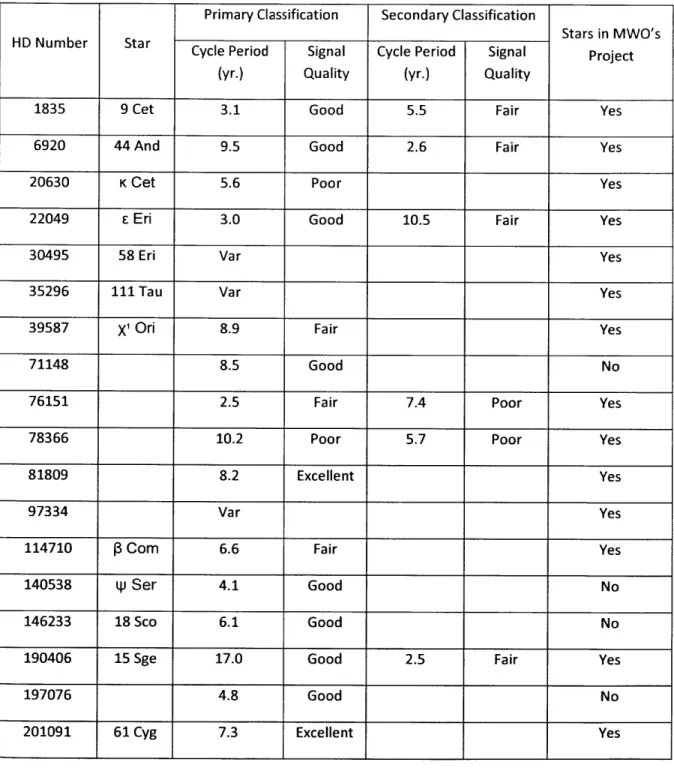
periodicity. The results are presented in Table 1 below. The short-period and long-period periodogram, created from SSS data, as well as the plot of S index as a function of time, using combined data from both SSS and MWO, for each star are also presented below (with the exception of HD 71148, HD 140538, and HD 146233, since they are not in the original MWO project). The FAP lines (50%, 10%, 1%, and 0.1%) are also included in each plot (Figure 3).
i5
10
20
15
10is
Period vs. Power Spectral Density, HD 35296
.. 000...
sn onono
5 10 152C
Pericc vs. Power Spectral Densfty, H D 35296
2' 1.4 1 2 101 a 6 25 0 0 40 60 so Period (days)
Perioc vs- Power Spectral Density, HD 35296
300 350
PerIod (days)
400
100
450
Figure 2. Power Spectral Density at three different timescales for HD 35296, showing dominant peaks at different regions. Three strong, well-defined peaks, where the power is unusually high, lie approximately at 1 day, 30 days, and 365 days, corresponding to the daily, monthly and annual peaks
10 al a,) a-_ ... ... ... t 0 0 2 -. . -. --.- - -...L0 0O~I -. ... n1000.... *1 onn -L
ilk
V
Table 1. Primary and Secondary Magnetic Activity Cycle of Stars and Their Signal Quality Primary Classification Secondary Classification
Stars in MWO's HD Number Sta r Cycle Period Signal Cycle Period
Signal Project
(yr.) Quality (yr.) Quality
1835 9 Cet 3.1 Good 5.5 Fair Yes
6920 44 And 9.5 Good 2.6 Fair Yes
20630 K Cet 5.6 Poor Yes
22049
E
En 3.0 Good 10.5 Fair Yes30495 58 Eri Var Yes
35296 111 Tau Var Yes
39587 X, Ori 8.9 Fair Yes
71148 8.5 Good No
76151 2.5 Fair 7.4 Poor Yes
78366 10.2 Poor 5.7 Poor Yes
81809 8.2 Excellent Yes
97334 Var Yes
114710
s
Con 6.6 Fair Yes140538 tp Ser 4.1 Good No
146233 18 Sco 6.1 Good No
190406 15 Sge 17.0 Good 2.5 Fair Yes
197076 4.8 Good No
400 0.50 D.45 s10 1.35 3.30 M*
b
20 Is o 600 W 1MISBOW
1000 ; iT
ST~T$ 199~
M 00 2005 oo 2010 o 2015,(> 1970 1976 1980 1 YearPeriod vs. Power Spectral DensIty, HD 920
200 401 000 Peftd (da4 to 15 0:1 0
Period vs. Power Spectral Density, HD 1835
I
*.1.ta
j
1 140.4203daye/
/
/
/
I ~4 1/. A 2000 4000 00 0000 Per id "Q 10000 985 1990Period vs. PowSpectal Deifty, HDOS6M
in o 5 -D. 1~# a000 000 02 0.24 0.22 S 0.20 0.18 0406
I
II2
0 I I 0 ]-2 0 11105 200O 2145 2010 2015 1970 1975 1980 1985 1990 YearFigure 3. Periodograms at two different timescales (0 -800 days and 800 - 8000 days) and plots of S index as a function of time for 18 stars in the SSS project. The S plots make use of both previous data by Baliunas et. al. from 1965 to 1992 (except for HD 71148, HD 140538, HD 146233, and HD 197076) as well as new data by SSS from 1993 to 2015.
12
a
14 12
Period vs Power Spectral Density, HD 1835
4IV IVv 2 "
...
.
/...
11
itT
1/I.
P*
jJuI
800 1000 0 2000 40M Pedod 0" V 9. .
:ft 6 1 A I I i A k 1 4 1 V I I a . . 4 1 . I . . 1-3e *
%
h
Period vs. Power Spectral Density, HD 20630
/0
15a
800 1000
Period 0eOel HD 20080 0.68 15 10 14 12 10 a 4 2 0Period vs. Power Spectral Density, HD 20630
2000 5m WW
5.6. fair
-a a a a I a a I a a a I a a a I a a a a1 a 1995
1970 1975 1960 1985 1990
Year
Period vs. Power Spectral Density, HD 22049
000
800
1000
Period (dy* 40 20 10 0 2000 2005 2010 2015Period v& Power Spectral Density, HD 22049
7
(3
18O.34deys ... * ... 0 2000 4000 POMO (dA) # 20040 .M ar .. -...1 1/
... ... l ...01
0 0.50 S 0.40 0.30d
30 20 RI 44 0.70 0.60 S 0 a000 8000 0 Period Jdays)Period vs. Power Spectral Density, HO 30495
...
...
47...
...
....
..
eOW W0 40 IS30 20 10 1000Period vs. Power Spectral Density, HD 30495
/
0 2000 4000 Period (d6ys OD 30405 0A03iT
~*
V-
10 00 205 2010 197" 1976 1980 198 1990 YearPeriod vs. Power Spectral Density, HD 35296
14 0 1flI fl A - IA/S /)0\ 4-2~, 400 Period (dos)
V
14 12 10 a 5Period vs. Power Spectral Density, HD 35296
10.WW 6 1000 100 200 3000 4000 s0m 6000 Period (day) HD 3590 0.m0 1I"#~h.sMum U
e
20 Is 10...
I0,\00
...
--
1-400 0.36 10,30 0.25f
12 10 86 4-2 LA I 0.46 0.40 S 0.30 0.25 W x 9 2000 2005 2010 201 1970 1975 1980 1905 1990 Year 5 14 9-Period vs, Power Spectral Density, HD 39587
I1 v
400 9W0 low100 .13111d duy*) 30 20 10 0 0Period vs. Power Spectral Density, HD 39587
- - - ... ----N -2000 4000 000 Pedod (dayo} HD 39M81 0.59 Yar 1970 1975 1980 1986 1990 Year
Period vs. Power Spectral Density HD 71148
10-2
0o
~7
400 0.185 0.1800.,175
0.1700.165
1000Period vs. Power Spectral Density, HO 71148
25 10.
v~\i"\
0 4 0 2000 4000 e0m 8000g
25-20 15' 040 S 0.35 0.30 026 8000 1000Kh
S -0- ---~
0 0 0~ RPeriod vs. Power Spectral Density, HD 76151
5t
0 6 400 $00 800 1000 Perid (ds 20 15 10 5 0Period vs. Power Spectral Density, HD 76151
. . . .
f... .
..
..
.
j A
/Vv...
i
....
..
...
...
...
0 2000 4000 Period (des) HD 76161 0.7, - T 995 2000 2W5 2010 1970 1975 1980 1985 1990 YearPeriod vs. Power Spectral Density, HD 78366
400 600 500 10CC
d d
0.30
025 0.20
Penod vs. Power Spectral Density, HD 78366
12-10 ---- - - - 4-2 0 2000 4000 Perod daya)
i
S 0.30 026 0.20 a000 000I
a000 0000 HD M 120 12.2 202 + .0 fair 1995 20WO 2M05 2010 2DI 16 1 I I 15Period vs. Power Spectral Density, HD 81809
12-\t
4 r 400 Goo $Do 1000 Psdod (dap) 40 30 0 a. 10 0Period vs. Power Spectral Density, HD 81809
A7 it / m ... ... C
...
0 2000 4000 PeWx (duys) e0m0 8000 HD S100 0.04 8 exat 1995 2000 2005 2010 2015 1970 1975 1980 Year 1905 1990Period vs. Power Spectral Density, HD 97334
S6440dap
...
...
i...
...
7 /-...
~
./..
...
C as 20 Is 10 0) 130D 2000 4000 Penad (ds) Poftd (day) SO am00 RD 97334 '''I r 0.61 J hA... 2000 2005 2010 2015k
0.22 0.20 0.14 0.10 0.14I
14 12 10 4 a 4 2 0 400Period vs. Power Spectral Density, HO 97334
- -tx/ 0.46 0.40 S 0.36 0.30 1065 1990
0
Yikr 9 T .. 19SPeriod vs. Power Spectral Density, HD 114710 400 D 000 POW Jdays) 31 ii 0 2000 4000 s000 Pesiod 0ay3) D 114110 0.67 16 good + OA fair Mt5 2000 2005 2010 2015 1970 1975 1980 1986 1990 Year
Period vs. Power Spectral Density HD 140538 20 4t is- 52O/ScaV 400 \ 00 100 so 40 s0 2D 10 0 0
Period vs. Power Spectral Density, HD 140538
LOOO
4000
PW"e (wey)
2010 2015 2020
18
m
Period vs. Power Spectrel Density, HO 114710/ / /
/
/ 2t~30.~l24'?d8~ / / / Ii / II I / -- H / 1O~(1.L~. ~A~N
V S 025 0.20 0.15 8000 10000n
S 0 25o
24 0,23 0.221 0.21 0. 8000 000 --, .- ., , I 0 0 t 2000 2005 Year . . . I I . W .5
Period vs. Power Spectral Density, HD 146233 f~ i 20 400 600 00 1000 Pedod (days)
.
195
0.190V
0.185
0.180
0.175
0.170
0.16[
2000
2005
Year a. 40Period vs. Power Spectral Density, HD 146233
n077 -Ays ... .... ... ... ... ... ... OL 0
2010
2000 4000 Pedod (days)2015
Period vs. Power Spectral Density, HD 190406
....
....
...
...
...
v ...
400 M30 S 0.20 WO Pdd(da) 800 so 40 20 0Period vs. Power Spectral Density, HD 190406
.... ....
-
---1000 0 2000 4000 s00 8000 Perod (day)0
0
2010 2015 0 S 6000 000p
m0 15 10 0 a-S 0 HD 190406 0.61 2.6. Iadr + 16.9 good 0'. Y Y I
1" 1-11
. . I
Period vs. Power Spectral Density, HD 197076 tam 170y0
..
.
..
.
..
.
.
.
L.
.
.
..
.
.
.
.
.
.
.
.
.
..
.
.
.
.
..
.
..
.
...
.
.
..
..
.
.
..
.
.
..
.
.
..
.
..
.
..
..
.
.
..
600 POW (days) 00 400 0 2 0. S 0 0-1 0. 1 25 20 1s 10 5 1000Period vs. Power Spectral Density, HD 197078
.. ..... ..... ..... ..... ..... ..... ..... ..... ..... ..... ..... ....
...
I
t.
...
-
...
...
0 2000 4000 Perod (day) m000 000 2 20~ 2005 2010 2015 2 YearPeriod vs, Power Spectral Density, HD 201091
M91W4dayu --- -.-.--- _/ 00 S00 PHod (dy) -. D 20001 1.10 7.3, exel - u,
Period vs. Power Spectral Density, HD 201091
0
-- I0-1000 0 2000 4000 000 Psod (days) [ I -, 1995 2000 2005 2010 2015 1970 1980 Year 1990 20q
12 10 a 6 4 2 Ar
30 25 20 15 10 5 0 30 1.0 0.8 0.6 0.4 00 im00:4 1 1
1 I I6
4COMPARISON WITH MWO RESULTS
Three notable regimes of stars arise as we compare these results to those by Baliunas et. al. They are discussed below.
* Stars with a strong degree of agreement
The most representative stars of this category are HD 81809 (Fig. 2k) and HD 201091 (Fig. 2r): there is very strong agreement between our data and MWO's data, both of which confirm a magnetic cycle of 8.2 years for HD 81809, and a cycle of 7.3 years for HD 201091. Furthermore, the cycles are clearly visible in the S index plots, with 'excellent' signal quality.
Additionally, our values for the two cycles of HD 190406 (Fig. 2p), 17 years and 2.5 years, are close to Baliunas et. al.'s corresponding results, 16.9 years and 2.6 years respectively. Our finding of HD 20630's cycle of 5.6 years (Fig. 2c) agree well with Baliunas et. al.'s earlier result as well.
Although no definite values could be determined for their cycle periods, our data and Baliunas et. al.'s for HD 30495, HD 35296 (Fig. 2e & 2f), and HD 97344 (Fig. 21) also agree that these three stars vary on long timescales without pronounced periodicity.
* Stars with a moderate degree of agreement
Our value of 2.5 years for HD 76151's short magnetic cycle (Fig. 2i) is also very close to Baliunas et. al.'s value of 2.52 years. However, we also detect a 'poor' signal of a 7.4-year cycle.
respectively). However, these cycles are not obvious in the plot of S index as a function of time, and there are noticeable differences between the trend of our data and that of Baliunas et. al.
* Stars with a strong degree of disagreement
HD 114710 (Fig. 2m) is one case where our results differ substantially from Baliunas et. al.'s. We find a magnetic cycle of 6.6 years, with fair signal. Baliunas et. al., however, derived two cycles of 16.6 years and 9.6 years. We are not able to reproduce the trend seen in the S index plot by Baliunas et. al.
Another case is HD 1835 (Fig. 2a), where we derive a primary activity cycle of period of
3.1 years, whereas the value by Baliunas et. al. was 9.1 years. Nevertheless, since the values are
near multiplicity of one another, it is possible that they represent the same signal. Part ofthe S index plot shows a recurring trend with a period of 9 years, but is not conclusive by itself.
* Stars not in MWO dataset
HD 71148 (Fig. 2h), HD 140538 (Fig. 2n), HD 146233 (Fig. 2o), and HD 197076 (Fig. 2q) each has one dominant magnetic cycle with periods 8.5 years, 4.1 year, 6.1 years, and 4.8
years, respectively.
STELLAR STATISTICS
The bar plot below show how the magnetic activity cycles of 18 stars in the SSS Project are distributed (Figure 4). The majority of the stars have cycles with period below 10 years. According to this plot, the Sun's 11-year sunspot cycle lies on the longer-period side of the plot, and thus is a rare occurrence among stellar population. However, there may be a selection bias, as the length of most data series is 20-25 year, which is not long enough to detect with certainty cycles with period longer than 10 years. More data are required to determine the actual
distribution of magnetic cycle periods, as well as how the Sun fits into the population of Sun-like
stars. This objective could be fulfilled by continuing observations in the future, or by combine
our data series with MWO's.
12 Distribution of cycle periods
10 8 E LI o 6 4 E z 2
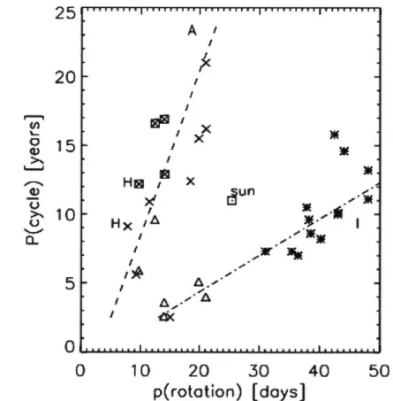
STELLAR DYNAMO AND THE ROTATION - ACTIVITY CYCLE RELATION
The theory of dynamo mechanisms as the driving force for stellar magnetic activity was reviewed extensively by Saar and Brandenburg (2000). In the paper, they note that the ratio of cycle frequency to rotational frequency increases with stellar chromospheric activity. In another paper, Saar and Brandenburg commented that stars generally follow two distinct sequences in the plot of stellar magnetic cycle periods as a function of rotational periods. They are called the active sequence (A) and the inactive sequence (I). The old, inactive stars on the I-sequence typically have Pcyc/Prot values 6 times larger than those of the young, active stars. To study the
empirical relations between the periods of activity cycles and rotational periods, Bohm-Vitense
(2006) used the same data from studies by Saar and Brandenburg (1999) and Lorente and
A x
20*
> 0 HXX15
0
10
20
30
40
50
p(rotation) [days]
Figure 5. Periods of activity cycles as a function of rotational periods. Reproduced from Bohm-Vitense (2006). Notice that there are two trends of magnetic activity, and that the Sun falls between them.
Montesinos (2005) to plot the periods of activity cycles as a function of rotational periods (Figure 5). This plot contains 8 out of 18 stars of the SSS project analyzed above, and it is apparent that stars follow two distinct trends as previously stated. (In the plot, "A" and "I" stand for active sequence and inactive sequence, respectively.)
We add the newfound results of 4 more stars (HD22049, HD39587, HD140538, and HD146233) to the plot, and confirm that they also lie on either of the sequences (Figure 6). Note
that several stars have two activity cycles lying on different sequences, namely HD 114710,
HD190406, and HD78366, which are in the SSS project, and HD22049, which we recently
25
20
0 015
10
A
x X.a E EA
-016
5
un
.'0
0
1020
30
40
50
p(rotat
o")
[days]
sun
In
I ~ I ~ V V I V I I ' & a & a L ..a d . - d . M .. .
added. The two activity cycles appear to work independently of one another. Durney et. al (1981) suggests that the secondary activity cycles of the A-sequence stars are generated in a different layer of the star than the first ones, meaning that there are multiple dynamos at work within a star. Bohm-Vitense comments that since most of the secondary cycles of the A-sequence stars fall on the I-sequence, it could be the case that the secondary activities of the A-sequence stars are generated by the same dynamo that is responsible for the primary activities of the I-sequence stars. They then put forth the hypothesis that different rotation velocity gradients, present in different stellar layers, contribute to different dynamos. Both kinds of dynamos can work simultaneously, but with different efficiency, creating two different sequences. For the A-sequence stars one dynamo is more efficient and for the I-A-sequence stars the other one is more efficient. The A-sequence stars also have many rotations per cycle (i.e. high Pcyc/Prot), suggesting that the dynamo works with relatively thin convection zones and small rotational gradients.
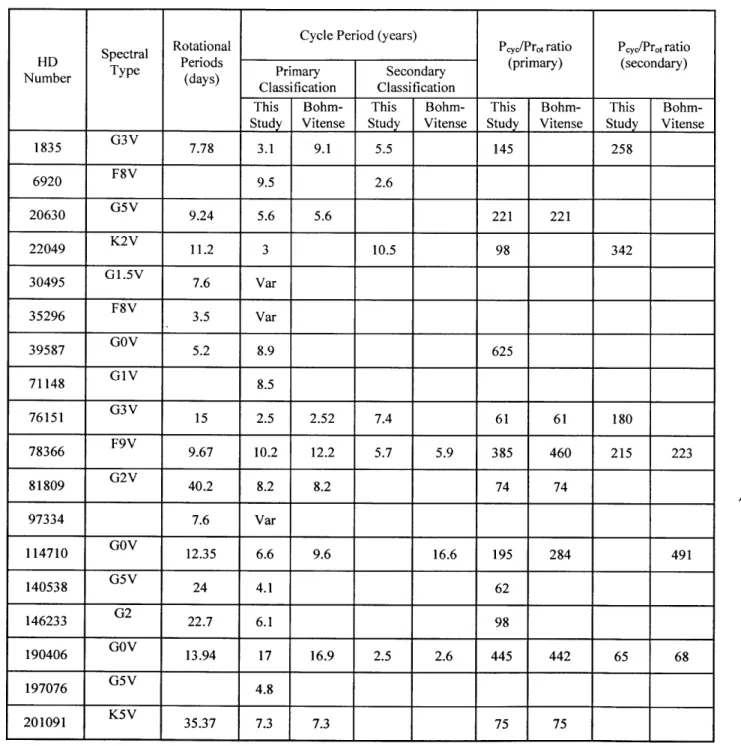
Table 3 summarizes our calculation of the ratio between the activity cycle periods and the rotational periods. The values from Bohm-Vitense were also included for comparison purpose. Unfortunately, for some stars the rotational periods are not known or exactly defined, so their ratio Pcyc/Prot is not known, nor can we place them on the plot by Bohm-Vitense. There are two distinct trends of values for Pcyc/Prot. Those on the I-sequence tend to have Pcyc/Prot in the range 60
- 120, whereas those on the A-sequence have values from 200 - 400, roughly 5 - 6 times larger.
In most cases, our derived values are close to those calculated by Bohn-Vitense. The table also includes spectral types of the stars in the population. However, there seems to be no correlation between stellar spectral type and magnetic cycle period.
Table 2. Cycle Periods, Rotational Periods, and The Ratio between them.
Spectral Rotational Cycle Period (years) Pcy,/Prt ratio Peyc/Prt ratio
HD Type Periods Primary Secondary (primary) (secondary) Number Te (days) Classification Classification
This Bohm- This Bohm- This Bohm- This
Bohm-Study Vitense Study Vitense Study Vitense Study Vitense
1835 G3V 7.78 3.1 9.1 5.5 145 258 6920 F8V 9.5 2.6 20630 G5V 9.24 5.6 5.6 221 221 22049 K2V 11.2 3 10.5 98 342 30495 GI.5V 7.6 Var 35296 F8V 3.5 Var 39587 GoV 5.2 8.9 625 71148 GIV 8.5 76151 G3V 15 2.5 2.52 7.4 61 61 180 78366 F9V 9.67 10.2 12.2 5.7 5.9 385 460 215 223 81809 G2V 40.2 8.2 8.2 74 74 97334 7.6 Var 114710 GOV 12.35 6.6 9.6 16.6 195 284 491 140538 G5V 24 4.1 62 146233 G2 22.7 6.1 98 190406 GOV 13.94 17 16.9 2.5 2.6 445 442 65 68 197076 G5V 4.8 201091 K5V 35.37 7.3 7.3 75 75 .1
THE SUN IN THE STELLAR CONTEXT
Interestingly, the Sun is among the very few stars lying in neither of the two sequences, indicating that it is not a good representative star for stellar magnetic discussion. This odd behavior, even among Sun-like stars, proves to be a problem, as the Sun is the only star whose many parameters can measured with certainty and monitored on long timescale. One hypothesis to explain the Sun's peculiarity is equally influenced by both kind of dynamos, instead of being dominated by one dynamo like the other stars (Bohm-Vitense, 2006). Another, suggested by Durney et. al. (1981), is that the Sun is transitioning from one sequence to another as its rotational velocity drops below a limiting value, causing the character of convection to change. Either case, it is reasonable to suspect that activity cycles are highly sensitive to stellar
parameters, and even a small deviation from solar parameters could result in behaviors drastically different from the Sun. This suggests that we may need to go further than the solar neighborhood in order to find a better sample of stars that behave more similarly to the Sun.
Currently, the SSS employs the 1.1-meter John Hall telescope at Lowell Observatory for data collecting purpose. The faintest stars that can be observed with high quality (i.e. signal-to-noise ratio) using this telescope have apparent magnitudes ranging from 6 to 7. In order to improve our sample pool, one direction we could take in the future is to employ a larger telescope. If we were to use the 4.3-meter Discovery Channel Telescope (DCT), also at Lowell Observatory, for the SSS project, the light-collecting area would increase by a factor of 15, extending the limiting apparent magnitude by 3. This means that we could observe faint Sun-like stars whose apparent magnitudes reaching 9 or 10, extending the sample pool of stars for our project by approximately 24 times.
CONCLUSION
Out of 18 stars taken from the SSS project and analyzed using the Lomb-Scargle method
of least-squares spectral analysis, 15 have well-defined magnetic activity cycles with periods ranging from 3 years to 20 years, whereas the remaining 3 stars appear to vary on timescales longer than the length of observation. Most of the derived values agree closely with previous results by Baliunas et. al.
We also add four more stars to the plot of activity cycle period - rotational period relation
by Bohm-Vitense, and they all lie on either the active sequence or the inactive sequence. This
result, together with the fact that several stars have two different cycles lying on different sequences, lends more evidence to the hypothesis that stars have multiple dynamos but are dominated by one of them.
The Sun, however, remains irregular even among Sun-like stars in its magnetic activity behavior. In order to understand better the position of the Sun in the stellar context, as well as details of dynamo mechanism inside the stars, it is necessary to continue observations of stars in the SSS project, as well as extend the sample pool by going further and searching for more Sun-like stars.
ACKNOWLEDGEMENT
REFERENCES
Baliunas et. al. (1994) Chromospheric Variations in Main-Sequence Stars. The Astrophysical Journal, 438
Baliunas et. al. (1996) A Dynamo Interpretation ofStellar Activity Cycles. The Astrophysical
Journal, 460
Bohm-Vitense, E. (2006) Chromospheric Activity in G & K Main-Sequence Stars and What It Tells Us About Stellar Dynamos. The Astrophysical Journal, 657
Hall J. & Lockwood G. (2004) The Chromospheric Activity and Variability of Cycling and Flat
Activity Solar-Analog Stars. The Astrophysical Journal, 614
Hall, J. & Lockwood, G. (2007) The Activity and Variability ofthe Sun and Sun-like Stars.
Synoptic Ca II H and K Observations. The Astronomical Journal, 133
Home & Baliunas (1986) A Prescriptionfor Period Analysis of Unevenly Sampled Time Series.
The Astrophysical Journal, 302
Metcalfe et. al. (2012) Magnetic Activity Cycles in the Exoplanet Host Star
E
Eridani. TheAstrophysical Journal Letters, 763
Saar, S. & Brandenburg, A. (1998) Time Evolution of The Magnetic Activity Cycle Period. The Astrophysical Journal, 498
Saar, S. & Brandenburg, A. (1999) Time Evolution of The Magnetic Activity Cycle Period II.
Result for an Extended Stellar Sample. The Astrophysical Journal, 524
Saar, S. & Brandenburg, A. (2000) Dynamo Mechanism. ASP Conference, 198
Scargle, J. (1982) Studies in Astronomical Time Series Analysis. Statistical Aspects of Spectral
Analysis of Unevenly Spaced Data. The Astrophysical Journal, 263
Wright et. al (2004) Chromospheric Ca II emission in Nearby F, G, K, and M stars. The Astrophysical Journal, Suppl. 152:261