Algorithms for autonomous urban navigation with formal specifications

Algorithms for Autonomous Urban Navigation

with Formal Specifications

by

Pratik Chaudhari

S. M., Massachusetts Institute of Technology (2012)

B. Tech., Indian Institute of Technology Bombay (2010)

Submitted to the Department of Aeronautics and Astronautics

in partial fulfillment of the requirements for the degree of

Engineer in Aeronautics and Astronautics

OF TECHNOLOGY

at the

_atthe

JUN

16

2014

MASSACHUSETTS INSTITUTE OF TECHNOLOGY

IOI

June

2014

LIBRARIES

© Massachusetts Institute of Technology 2014. All rights reserved.

Author ...

Sa

..

Department of Aeronautics and Astronautics

May 22,2014

Certifiedby

...

Signature redacted

'Emilio Frazzoli

Professor of Aeronautics and Astronautics

Thesis Supervisor

Certified by

...

Signature redacted

Sertac Karaman

Assistant Professor of Aeronautics and Astronautics

Thesis Committee Member

Accepted by

...

Signature redacted

-Paulo C. Lozano

Associate Professor of Aeronautics and Astronautics

Chairman, Graduate Program Committee

Algorithms for Autonomous Urban Navigation

with Formal Specifications

by

Pratik Chaudhari

Submitted to the Department of Aeronautics and Astronautics on May 22, 2014, in partial fulfilment of the

requirements for the degree of Engineer in Aeronautics and Astronautics

Abstract

This thesis addresses problems in planning and control of autonomous agents. The central theme of this work is that integration of "low-level control synthesis" and "high-level decision making" is essential to devise robust algorithms with provable guarantees on performance.

We pursue two main directions here. The first part considers planning and control algorithms that satisfy temporal specifications expressed using formal languages. We focus on task specifications that become feasible only if some of the specifications are violated and compute a control law that minimizes the level of unsafety of the system while guaranteeing that it still satisfies the task specification. Examples in this domain are motivated from an autonomous car navigating an urban landscape while following road safety rules such as "always travel in the left lane" and "do not change lanes

frequently" or an electric vehicle in a mobility-on-demand scenario.

The second part of the thesis focuses on multi-agent control synthesis, where agents are modeled as dynamical systems and they interact with each other while sharing the same road infrastructure - all the while respecting the same road driving rules expressed as LTL specifications. We discuss algorithms that identify well-defined no-tions in the game theory literature such as Stackelberg equilibria and non-cooperative Nash equilibria under various information structures.

This work builds upon ideas from three different fields, viz., sampling-based motion-planning algorithms to construct efficient concretizations of general, continuous time dynamical systems, model checking for formal specifications that helps guarantee the safety of a system under all scenarios, and game theory to model the interaction be-tween different agents trying to perform possibly conflicting tasks.

Thesis Supervisor: Emilio Frazzoli

Title: Professor of Aeronautics and Astronautics Thesis Committee Member: Sertac Karaman

Acknowledgments

I would like to express my gratitude to my advisor, Emilio Frazzoli. I have benefited

im-mensely from his unwavering belief in his students along with his vision and amazing ability to identify important problems. He has been invaluable as a mentor and I consider myself extremely lucky to have been able to work closely with him. I would like to thank Sertac Karaman who is also my committee member on this thesis. Long conversations with him have had a huge impact in shaping my thinking as a young graduate student and he continues to be an enormous source of inspiration.

I have been lucky to be taught by some truly legendary teachers here at MIT. Their style and

depth of knowledge is something I aspire to emulate. I dream of becoming a professor one day and

I could not have wished for better role models. Being at LIDS has been instrumental in channeling

my research interests. It has expanded my knowledge and broadened my horizons.

I have been lucky to work with a number of wonderful collaborators in the past few years. In

particular, I would like to thank David Hsu at the National University of Singapore, Nok Wong-piromsarn at the Singapore-MIT Alliance for Research and Technology and Jana Tumova at the Royal Institute of Technology. Many a time, they have humored me and lent a patient ear to my half-baked ideas to help me evolve them into the material presented here. A special thanks goes to

Jana

who first introduced me to some of the most beautiful material in computer science that forms the crux of this thesis. She is a rare person and I have greatly enjoyed working with her. Luis Reyes-Castro and Valerio Varricchio with whom I worked closely in Singapore, have become fast friends.

I am fortunate to have several friends who have made this journey enjoyable and memorable. I would like to thank my lab mates at ARES and SMART for the amazing times we have shared.

Here's to all the Dungeons and Dragons and the endless nights spent in the by-lanes of Singapore!

I would also like to thank all the friends I have made at Cambridge and MIT, quite a few of them

are old friends whom I have known for almost a decade. Graduate school so far away from home would not have been as enriching or fulfilling without them. I will cherish these memories.

Lastly, I would like to thank my parents and my brother. No words can do justice to all the sac-rifices they have made for me. They have been a constant source of strength and encouragement, without which this thesis would have been impossible.

Contents

Page

Introduction

Motivation and Contributions

Organization

Published Results

Background Material

Durational Kripke Structures for Dynamical Systems

Linear Temporal Logic (LTL)

Process Algebras

Differential Games

Minimum-violation Planning

Level of Unsafety

Problem Formulation

Algorithm and Analysis

Experiments

Process Algebra Specifications

Problem Formulation

Algorithm

Experiments

Multi-agent Systems

Problem Formulation

Stackelberg Games: Algorithm and Analysis

Non-cooperative Games

Experiments

Conclusions and Future Directions

Chapter 1

1.1

1.2

1.3

Chapter 2

2.1

2.2

2.3

2.4

Chapter 3

3.1

3.2

3.3

3.4

Chapter 4

4.1

4.2

4.3

Chapter 5

5.1

5.2

5.3

5.4

Chapter 6

9

10

12

13

14

14

16

20

21

23

23

24

25

29

35

36

38

39

43

44

46

49

53

56

CHAPTER

1

Introduction

From avoiding traffic jams in busy cities to helping the disabled and elderly on their daily commute, autonomous vehicles promise to revolutionize transportation. The DARPA Grand Challenges [L .T 08, 131S09, TMD 06]

were a gigantic leap towards this goal when they demonstrated that self-driving cars can not only traverse unknown terrain but can also do well in an urban scenario, complete with traffic rules. However, as autonomous cars

begin their transition from these experimental Figure 1.: MIT's DARPA Urban Challenge car projects into viable means of urban

transporta-tion, we are faced with a myriad of challenges, e.g., traffic management for autonomous cars, interaction of these agents with other drivers, sharing road infrastructure with pedestrians etc.

- and most importantly, doing so while maintaining the same standards of safety that human drivers are subject to.

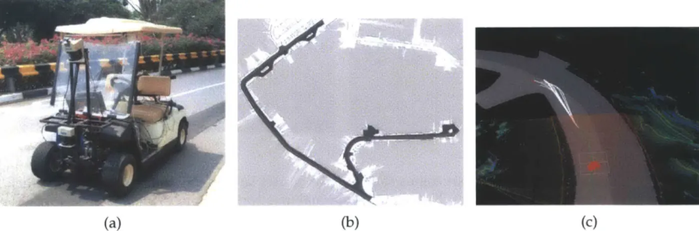
To motivate the problems considered in this thesis, let us look at the DARPA Urban Challenge of 2007. It required competing teams to traverse an urban landscape in a completely autonomous manner. Doing so involved performing challenging tasks such as parking maneuvers, U-turns and negotiating cross-roads - all the while obeying traffic regulations. Fig. 1.1 shows Talos, MIT's entry to this competition, which is an LR3 Landrover outfitted with 5 cameras, 12 LIDARs, 16 radars and one 3D laser (Velodyne) sensor. The computing system on the other hand consists of a few hundred processes running in parallel on 40 processors. Team MIT was placed fourth in this competition and it completed an approximately 60 mile route in about 6 hours.

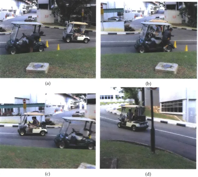
Fig. 1.2 shows a picture of the sensory and control data when Talos encounters Cornell University's car (Alice). Alice unfortunately has a bug in the software which causes it to stall in the middle of the road. After waiting

for

some time for Alice to make progress, Talos plans an alternate trajectory around it. How-ever, as Talos gets closer to Alice, a

fail-safe

mechanism in Alice kicks in which says that it should not be very close to another vehicle

and Alice moves forward. By this time how- Figure 1.2: Cornell-MIT crash ever, both cars are committed to their

respec-1.1 MOTIVATION AND CONTRIBUTIONS

tive

fail-safe

trajectories and they end up colliding. This incident - and a number of similar ones happened to almost all teams - provides the main motivation for this thesis. Specifically, we identify the following key points that resulted in the collision [FBI 08]:

1. An alternate trajectory that was classified as "safe" by Talos transitioned from the left-lane

into the right-lane, which is a potentially dangerous maneuver, in other words, high-level rou-tines that reason about logical safety of a trajectory were completely decoupled from motion-planning.

2. Alice had a number of conflicting

fail-safe

rules whose priorities were not clearly defined with respect to each other. In particular, even though, each of them guaranteed reasonable behavior individually, together, they were not able to guarantee the vehicle's safety.

3. Talos did not correctly judge the intent of the other vehicle, i.e., sensory information and

per-ception algorithms were insufficient to classify Alice as "another car that is likely to move". Let us elaborate further on these points. In the next section, we will identify some fundamental challenges in traditional engineering methodologies for such systems.

1.1 Motivation and Contributions

1.1.1 Integrated Decision Making and Control

One of the main challenges of reasoning about "high-level decision making" and implement-ing it usimplement-ing "low-level controllers" is that the computational models at these two levels are incompatible. For example, logical rules like "do not go into the left lane" that can be eas-ily verified for discrete state-trajectories are hard to verify (or even formalize) for dynam-ical systems with differential constraints. This has led to a hierarchy of design methodologies wherein, tools from computer science and con-trol theory respectively, are used independently of each other. While this is both reasonable and effective, one of the main challenges of this ap-proach is that evaluating the performance or proving the safety of the closed-loop system with respect to its specifications, is difficult. In fact, if the abstracted finite transition system is too coarse, there is no guarantee that the op-timal controller will be found even if one ex-ists [WTM 10], i.e., these methods are not com-plete and cannot be applied to, for example, dynamically changing environments.

In this work, we propose an integrated ar-chitecture for decision making and control. We

Figure 1.3: The first picture shows the left lane as a "virtual obstacle". If no progress is made for 15 secs., as shown in the second picture, the software clears the left-lane and allows the car to overtake a parked car.

1.1 MOTIVATION AND CONTRIBUTIONS

construct on line sequences of concretizations of general, dynamical systems known as Kripke structures that also maintain low-level control laws. These Kripke structures are finite models of the continuous dynamical system and algorithms from model checking in the computer sci-ence literature can be readily used to evaluate temporal properties such as safety, fairness, live-ness and their combinations. Also, we are interested in refining these Kripke structures to obtain asymptotic-optimality of the resulting algorithms. In order to differentiate this fromfinite

abstrac-tions that are popular in literature, we call these, concretizaabstrac-tions of dynamical systems.

This thesis proposes a way to construct concretizations of dynamical systems with differen-tial constraints. We use ideas from sampling-based motion-planning algorithms such as Prob-abilistic Road Maps (PRMs) and Rapidly-exploring Random Trees (RRTs) to create iteratively refined Kripke structures. In particular, recent versions of these algorithms such as PRM* and RRT* [KF1 1b] help us ensure two important characteristics that differentiate this work from con-temporary results, (i) probabilistic completeness, i.e., the algorithm finds a Kripke structure that satisfies the specifications if one exists with high probability, and (ii) probabilistic asymptotic-optimality, i.e., almost surely, the algorithm returns a continuous trajectory that not only satisfies all specifications but also minimizes a given cost function while doing so.

1.1.2 Minimum-violation Planning

Logical specifications can be succinctly expressed using formal languages such as Linear Tem-poral Logic (LTL) [KB06, KGFP07], Computational Tree Logic (CTL, CTL*) [LWAB10], modal y-calculus [KF 12a] etc. The general problem of finding optimal controllers that satisfy these speci-fications has been studied in a number of recent works such as [DSBR11,T1P06,STBR1 1, USDB12]. Given these specifications, if the underlying task is feasible, using methods discussed in the pre-vious section, we can compute an asymptotically-optimal controller for a given dynamical system that satisfies them. On the other hand, in many situations, for example when a single-lane road is blocked, one might have to violate some specifications, e.g., "do not go into the left lane" in order to satisfy the task, e.g., "reach a goal region". In fact, (cf. Fig. 1.3), MIT's DARPA Grand Challenge team had a series of rules in their code to demarcate the left-lane as a virtual "obstacle"; if no progress was made for 15 secs. due to a blocked right lane, the algorithm would selectively remove these "obstacles" until a reasonable motion-plan was found. A consequence of this is that a number of such conflicting rules and pre-specified parameters exist in the framework which makes it very hard to design and debug. It is also hard to guarantee the performance and safety of the overall system.

This thesis discusses a principled approach to tackle such problems. In particular, in our work, we quantify the level of unsafety of a trajectory that breaks a subset of specifications in order to satisfy a task. These specifications are expressed using the finite fragment of LTL, e.g., FLTL_ x, and are converted into a weighted finite automaton such that traces of the Kripke structure on this automaton have a weight that is exactly equal to the level of unsafety of the corresponding trajectory Using ideas from local model-checking and sampling-based motion-planning, we can then construct an algorithm that identifies the trace in the Kripke structure (and effectively, the continuous trajectory) that minimizes this level of unsafety.

Our work here can be seen in context of recent literature on control synthesis for an unsatisfi-able set of specifications. For example, works such as [CRST08] reveal unsatisfiunsatisfi-able fragments of given specification, while others such as [Fa i1, KFS 12, KF 12b] try to synthesize controllers with minimal changes to the original specifications, e.g., by modifying the transition system. Two

1.2 ORGANIZATION

lines of work that are closest to ideas proposed in this thesis are - [Hau 12] which focuses on finding the least set of constraints, the removal of which results in satisfaction of specifications and [DF1 1, CY98] which quantify the least-violating controller according to some proposed metric for a given transition system. Let us note that similar approaches exist for probabilistic transition systems, e.g., [BEGL99, BGK 11,].

1.1.3 Multi-agent Systems

On the other hand, consider problems such as merging into lanes on freeways, negotiating cross-road junctions, round-abouts etc. In order to enable autonomous vehicles to reason about these situations effectively, we have to develop algorithms for interaction of these agents with the ex-ternal environment. This thesis takes a look at game theoretic approaches to these problems in conjunction with concepts from model checking and sampling-based algorithms.

Differential games [Isa99,B095] are popular models for problems such as multi-agent collision avoidance [MBT05], path planning in adversarial environments [VBJPI,0] and pursuit-evasion problems [GLL I _{99]. However, analytical solutions for differential games exist for only specific}

problems, e.g., the "lady in the lake" game, or Linear Quadratic Regulator (LQR) games [B095]. For problems involving more complex dynamics or other kinds of cost functions, solutions are hard to characterize in closed form. Numerical techniques are based on converting the problem to a finite dimensional optimization problem [RaiO ] or solving the corresponding partial differ-ential equations using shooting methods [BPG93, BCD97, BFS99,Sou99], level set methods [Set96], viability theory [ABSPI1, CQSP199] etc.

Similarly, there are few rigorous results for game theoretic controller synthesis for multi-robot planning, e.g., [LH98]. However, a number of works solve related problems, e.g., [ZM13] solves optimal sensor deployment while [ASF09] considers vehicle routing problems. These papers mainly reply on centralized planning [SL02, XA08], decoupled synthesis [KZ86, SLL02] or ad-hoc priority-based planning, e.g., [Buc89, E LP87].

This thesis proposes a formulation to compute equilibria for two-player differential games where players try to accomplish a task specification while satisfying safety rules expressed using temporal logic. We formulate the interaction between an autonomous agent and its environment as a non-zero sum differential game; both the robot and the environment minimize the level of unsafety of a trajectory with respect to safety rules expressed using LTL formulas. We describe an algorithm to compute the open-loop Stackelberg equilibrium (OLS) of this game. We also consider generic motion-planning tasks for multi-robot systems and devise an algorithm that converges to the non-cooperative Nash equilibrium of the differential game in the limit. Throughout, we em-ploy techniques from sampling-based algorithm to construct concretizations of dynamical systems (cf. Sec. 1.1.1) and model checking techniques on these Kripke structures.

1.2 Organization

This document is organized as follows. In Chap. 1, we develop some preliminary concepts that are used in the remainder of the thesis. We construct durational Kripke structures for efficient model checking of dynamical systems and provide an overview of Linear Temporal Logic (LTL) along with automata based approaches for model checking LTL. This chapter also introduces process algebras and develops various preliminary concepts for differential games.

1.3 PUBLISHED RESULTS

Chap. 3 formulates the problem of "minimum-violation motion-planning" and proposes an algorithm that minimizes the level of unsafety of a trajectory of the dynamical system with re-spect to LTL specifications. It also provides a number of results from computational experiments along with an implementation on an experimental full-size autonomous platform. Chap. 4 de-velops these concepts further, but takes a different route. It considers specifications which can be expressed using simple languages such as process algebras and finds a number of applications related to mobility-on-demand that can be solved using these.

Chap. 5 delves into multi-agent motion-planning problems. It first formulates a two-player, non-zero sum differential game between the robot and external agents and proposes an algorithm that converges to the Stackelberg equilibrium asymptotically. The central theme of this chapter is that we incorporate "minimum-violation" cost functions into game theoretic motion-planning. The later part of his chapter uses ideas from sampling-based algorithms to look at n-player non-cooperative Nash equilibria for generic motion-planning tasks.

Finally, we take a holistic view of urban motion-planning using formal specifications and com-ment on future directions for research.

1.3 Published Results

Parts of this thesis have been published in the following research articles

-1. Luis I. Reyes Castro, Pratik Chaudhari, Jana Tumova, Sertac Karaman, Emilio Frazzoli, and Daniela

Rus. Incremental Sampling-based Algorithm for Minimum-violation Motion Planning. In Proc. of IEEE

International Conference on Decision and Control (CDC), 2013.

2. Valerio Varricchio, Pratik Chaudhari, and Emilio Frazzoli. Sampling-based Algorithms for Optimal

Motion Planning using Process Algebra Specifications. In Proc. of IEEE Conf. on Robotics and Automation,

2014.

3. Minghui Zhu, Michael Otte, Pratik Chaudhari, and Emilio Frazzoli. Game theoretic controller synthesis

for multi-robot motion planning Part I: Trajectory based algorithms. In Proc. of IEEE Conf. on Robotics and Automation, 2014.

4. Pratik Chaudhari, Tichakorn Wongpiromsarn, and Emilio Frazzoli. Incremental Synthesis of Minimum-Violation Control Strategies for Robots Interacting with External Agents. In Proc. of American Control

CHAPTER

2

Background Material

This chapter introduces some preliminary material on dynamical sys-tems with differential constraints and Kripke structures which are effi-cient data-structures to talk about temporal properties of trajectories of dynamical systems. It also introduces formal languages such as Linear Temporal Logic and Process Algebras and model checking algorithms for these languages that are used in this work. Lastly, we provide some dis-cussion on game theoretic notions of equilibria such as the Nash equilib-rium and Stackelberg equilibequilib-rium under various information structures.

Notation: For a finite set S, denote the cardinality and the powerset of S as

ISI

and 2s, re-spectively. Let S * be the set of all finite sequences of elements of S and for u, v E S*, denote the concatenation of u and v as u - v. Let S' denote the set of all infinite strings of elements of S and given some u E S*, we denote by uW E S', its infinite concatenation with itself.

2.1 Durational Kripke Structures for Dynamical Systems

Consider a dynamical system given by

(t) =

f(x(t),ut)),

x(0) = xinit, (2.1)

where x(t) E X C Rd and u(t) E U C R'n with X,U being compact sets and xinit is the initial state. Trajectories of states and control are maps x : [0, T] -* X and u : [0, T] -+ U respectively

for some T E R>0. We will tacitly assume in all this work that the above equation has a unique

solution for every xinit; in order to do so, we assume that

f(,

)

is Lipschitz continuous in both its arguments and u is Lebesgue measurable.

Let H be a finite set of "atomic propositions" and L: X - 211 map each state to atomic propositions that are true at that state. We can reason about the atomic propositions satisfied by a trajectory of the dynamical system as follows. For a trajectory x, let D(x) = {t I2L(x(t)

#

limest-

ICJ(x(s)),O

< t < T} be the set of all discontinuities of Lc(x(.)). In this work, we assume

that D (x) is finite for all trajectories. This is true for various different Les considered here, one can show that the set of trajectories that do not satisfy this condition has measure zero. A trajectory x: [0, T] -* X with D(x) = {t1,.. , tn} produces afinite timed word

Wt = (to,do),(fld1),..., Vn, dn), where

(i) Ck = Ic(x(tk))

for all 0

<

k < n and to

=

0,

dk = tk+1 - tk

and

(ii) fn = Lc(x(tn)) and dn = T - tn.

2.1 DURATIONAL KRIPKE STRUCTURES FOR DYNAMICAL SYSTEMS

Thefinite word produced by this trajectory is

w(x) = to, ,-, .

We are now ready to define a special type of Kripke structure that allows us to reason about all timed words produced by a dynamical system.

Definition 2.1 (Durational Kripke structure). A durational Kripke structure is defined by a tuple K = _{(S, sinit, R, I, L, A), where S is a finite set of states, sinit E S is the initial state, R} C S x S is a deterministic transition relation, 1-I is the set of atomic propositions, L : S -+ 211 is a state labeling function, and A : R -+ R>o is a function that assigns a time duration to each transition.

A trace of K is a finite sequence of states p = so, si, ... , s, such that so = sinit and (sk, Sk+1) E

R for all 0 < k < n. Corresponding to it is the finite timed word that it produces, i.e., pt (to,,do),(f,d1),..., fn,dn) where (fk,dk) = (L(sk), A(sk,sk+1)) for all 0 < k < n and (Ln,dn)

(L (sn), 0). The word produced by this trace is w(p) = to, f1, . . ., fn. Note that as defined until now,

a word may have multiple consecutive 4ks that are the same, e.g., the trajectory spends a lot of time in each labeled region. Such repeated atomic propositions are not useful to us for reasoning about temporal properties of the trajectories and hence we remove them using the destutter operator as shown below.

Given w(p), let I = {io, i, .. ., ik} be the unique set of indices such that io = 0 and

fii = ii+1 =. -- ii£_ : fi1 for all 0 j < k - 1

and similarly k = - -- = en. Define the "destutter" operator to remove these repeated

consecutive elements of a word as

destutter(W(p)) = fyi, fil, ... ., fik_ , tik.

For convenience we also denote the duration of a trace by (p), i.e., (p) = En o di. Let us now define a Kripke structure that explicitly encodes the properties of the dynamical system under consideration.

Definition 2.2 (Trace-inclusive Kripke structure). A Kripke structure K = (S, sinit, R, I, L, A) is

called trace-inclusive with respect to the dynamical system in Eqn. (2.1) if * S C X, Sinit = Xinit,

* for all (s1,s2) E R there exists a trajectory x : [0, T] -+ X such that x(0) = si and x(T) S2 with T = A(sI,s 2) and ID(x)| I 1 i.e., L,(x(.)) changes its value at most once while

transitioning from s1 to S2.

The following lemma now easily follows, it relates trajectories of the dynamical system to traces of a trace-inclusive Kripke structure.

Lemma 2.3. For any trace p of a trace-inclusive Kripke structure, there exists a trajectory of the dynamical system, say x : [0, T] -+ X such that

2.2 LINEAR TEMPORAL LOGIC (LTL)

2.2 Linear Temporal Logic (LTL)

We start by defining a finite automaton. For a more thorough and leisurely introduction to the theory of computation and temporal logics, one may refer to a number of excellent texts on the subject, e.g., [Sip12, BK : 08].

Definition 2.4 (NFA). A non-deterministic finite automaton (NFA) is a tuple A = (Q, qinit, E, 5, F)

where Q is a finite set of states, qinit E

Q

is the initial state, E is a finite set called the input alphabet,

5

C

Q

x E x

Q

is a non-deterministic transition relation and F C

Q

is a set of accepting states. The semantics of finite automata are defined over E*, in particular traces of Kripke structures.

A run p of a finite automaton for the input - =- i, o2, . . ., o-, is the sequence qo, q1, ... , qn such that

qo

= _{qinit, (qk-1, o-k, qk) E 6 for all k < n. We say that the input o- is accepted if qn E F and rejected}

otherwise. The set of all finite strings accepted by an NFA is called its language.

If the transition relation is deterministic, i.e., each state in the automaton can transition to only

one other state, we say that A is a deterministic finite automaton (DFA). It is surprising that we do not gain any expressive power by non-determinism in finite automata, in other words, the set of all languages that can be expressed using NFAs - also called regular languages - is exactly the same as the set of all languages expressed using DFAs. Consequently, any NFA can be converted into a DFA (possibly, with exponentially many states) having the same language.

In the context of this work, NFAs will have an input alphabet of 2-tuples, consecutive elements of the word produced by a trace of the Kripke structure will form the input alphabet. Thus, if

a- =

(k,

fk+1) for some k, we have E = 2 x _{2n. Using this, we can talk about NFAs which "detect}

the change" in the logical properties of a trajectory. As a technicality, we will also require NFAs to be non-blocking, i.e., for all states q E

Q,

and a E E, there exists a transition (q, o-, q') C ( for some q' E

Q.

Note that any blocking automaton can be trivially made non-blocking by adding transitions to a new state qnew j F.

Definition 2.5 (w-automaton). An w-automaton is a tuple A = (Q, qinit, E, (, Acc) where the ele-ments

Q,

_{qinit, E and ( are the same as an NFA and Acc is an "acceptance condition".}

The semantics of w-automata are defined similarly as NFAs, except that they are over infinite input words, i.e., elments of El. We thus need to re-define what it means for an w-automaton to "accept" a word, which brings us to the acceptance condition. Contrary to NFAs and DFAs, a number of different accepting conditions give rise to w-automata of varying power. For a Buchi automaton (BA), Acc is "for a given set F C

Q,

a run p is accepted if it intersects F infinitely many times". For a generalized Buchi automaton (GBA), Acc is "given {F1, F2... , Fm} Q Q', a

run p is accepting if it intersects each Fi infinitely many times". In addition to this, there are a number of other w-automata with different accepting conditions such as Muller, Rabin, Streett and parity automata. We note here that in the world of w-regular languages, i.e., languages of w-automata, non-determinism is powerful. Non-deterministic BAs, even deterministic Rabin and Muller automata can all be shown to express the whole set of w-regular languages; on the other hand deterministic BAs only express a strict subset of w-regular languages.

We will not be using w-automata in this work. We however motivate model-checking for Linear Temporal Logic, which is a strict subset of w-regular languages using these concepts.

2.2 LINEAR TEMPORAL LOGIC (LTL)

2.2.1 Syntax and Semantics of LTL

Temporal properties can be expressed using w-automata as we saw earlier. However, there are more concise representations using languages that are also easy to read for humans. Proposi-tional LTL is one such language - it appends propositional logic with temporal operators. LTL is defined inductively and the syntax can be given by the following grammar:

P ::= true

a 1P1 A P21 X

' I11

U 02

where a E 1I. Using these we can define temporal modalities like F (eventually) and G (always) as follows:

F'P==trueU'P GP=,(FP)

i.e., if it never happens that

-,P

is true eventually, then

P

always holds, equivalently

P

holds from

now on forever. The semantics of LTL can be defined as follows. Given 0 =_ Oi ... E EF, we

denote the (infinite) substring from element j as crU.] = o-jj+. ... Then

o-

@

true

c- a iff o-o a

O~

'P A 2 iff

o-

Pland

o-

u 2

-1 P iff L-o V P

0b X P iff T[1i: ]P

U~ #P1 U 2 iff 3 j > 0, j:]

I=

02and oi: kP i V 0 < i < j

LTL can be used to succinctly express various temporal properties, for example, * liveness: G F

P

(P holds infinitely often),

*

safety: G

-,P

(avoid

P),

* reactivity: G F '1 -> G F '2 (if 'P holds infinitely often, so must 02) etc.

In order to verify if traces of a Kripke structure satisfy the temporal properties denoted by a given LTL expression

',

we use automata-based model checking, i.e., the LTL expression is first converted into an equivalent w-regular automaton. Using algorithms discussed in Sec. 2.2.2, we can then use simple search algorithms to verify '. Here, we briefly discuss the conversion of

LTL to Buchi automata [VW94]. Assume that the formula is in negated normalform. We construct the closure of 0, denoted as cl(P), which is the set of all sub-formulas and their negations. Not surprisingly, this forms the alphabet the Buchi. The states of the Buchi are the maximal subsets of cl(P), i.e., largest sets of formulas that are consistent. Roughly, for a state q c M C cl(P) of the

GBA, there exists an accepting run of the automaton that satisfies every formula in M and does not

satisfy any formula in cl(P) \ M. The transition function is easy to construct, we just don't have to violate any temporal or Boolean properties of LTL while connecting two states. The accepting states are Fp for every sub-formula of the form p = '1 U '2 of P. We ensure that for a run BOB₁... , if

ip

E B0, we have that '2 E B1 for some j > 0 and 'P E Bi for all i <

j.

The acceptance condition is

thus a GBA condition. This automaton can be easily de-generalized into an NBA using standard algorithms [BK 08].

As an interesting aside, let us note that since deterministic Buchi automata cannot exhaust w-regular properties, we cannot use automata minimizing algorithms to convert NBAs to DBAs.

2.2 LINEAR TEMPORAL LOGIC (LTL)

This is particularly important because the size of NBA constructed above is exponential in the size of

q

and the size of model checking is proportional to the size of the NBA.

Finite Linear Temporal Logic (FLTL)

We focus here on temporal properties expressed using the finite fragment of LTL. Finite LTL [MP95,

GP02] has the same syntax as LTL with the semantics defined over finite runs of the underlying

transition system. FLTL is defined using two kinds of X operators, the strong next operator, de-noted using the usual X says that a property

q

is true in the next time instant. Of course, since FLTL deals with finite strings, there is no way this property can be true at the last instant. Hence, we define a weak next operator, denoted as X which says that 0 is true in the next instant if one exists. This also gives rise to a corresponding weak until operator.

Let us now present the construction of NFAs from FLTL specifications. Please refer to [GPO2] for a more elaborate discussion. Because there does not exist an equivalent "generalized NFA", we use a slightly modified version of the LTL conversion algorithm as shown here [GPVW95]. For a negated normal formula

p,

construct a graph where each vertex v holds the following data:

" id: a unique identifier,

* incoming: the set of edges that point to v,

e new: sub-formulas which hold below v but are not yet processed,

" old: sub-formulas which hold below v that are processed,

* next: sub-formulas that have to hold for all successors of v,

" strong: a flag to signal that v cannot be the last state in a sequence.

The algorithm then

con-structs a graph G starting

from a vertex v, which has Formula left new left next strong right new right next incoming from a dummy y

U

v Y y

U

v 1 v 0

vertex init, with new = y UV v U V Y, v 0

{p}

and old, next = 0. YV v Y 0 v 0

Initialize an empty list called y A v Y, v 0 -

-completed-nodes. Recur- X 0 p -

-sively, for a node v not yet X 0 p 1 -

-in completed-nodes, move p/,p

0

0

-

-a sub-formul-a rj from new

to old. Split v into left _{Figure 2.1: Table for branching in conversion of FLTL to NFA} and right copies according

to Tab. 2.1. old, incoming retain their values. Roughly, the strong indicates that the formulas in next are to be upgraded from weak next to strong next.

If there are no more sub-formulas in new of v, compare v to completed-nodes to check if there is some node u that has the same old and next and add incoming of v to incoming of u, i.e., there are multiple ways of arriving at the same u. Else, add v to completed-nodes and start a new node's recursion with an incoming edge from v and its new is the next of v.

The states of the NFA are then all the nodes in the list of completed nodes. The initial nodes are the ones with incoming edges from init. The transition relation is easily obtained from incoming.

2.2 LINEAR TEMPORAL LOGIC (LTL)

To get the accept states, note that a state is an accept state iff for each sub-formula of

q

of the form p U v, either old contains v or it does not contain y U v and its strong bit is set to false.

As an important deviation from conventional FLTL, in our work, we would like to reason about the properties of a trajectory of a dynamical system, i.e., w(x). Thus, we do not use formulas which involve the X operator and define FLTL_ x to be FLTL without the X operator.

2.2.2 Model Checking LTL and its Variants

To motivate automata based model checking for LTL, let us first consider verification of safety properties which are regular languages. Let us consider the complement of this set, i.e., all the bad finite strings. It is easy to see that we need only work with the "minimal" such set, i.e., the smallest set of bad prefixes. Since this by assumption is a regular language, we can find an automaton A that accepts all minimal bad prefixes. Given a Kripke structure K, the problem is then to find whether there exists a trace of K that is accepted by A. This can be posed as simple reachability problem on the "product automaton" defined as follows:

Definition 2.6 (Product automaton). Given a Kripke structure K = (S, sinit, R, 1I, L, A) and a non-blocking finite automaton A, the product automaton is a tuple P = K 0 A = (Qp, qinit,p, 211, 6p, Fp)

where

SQP

= S X Q,

qinitP = (sini , qinit) is the initial state,

e

cp

C Qp x Qp is non-deterministic transition relation such that ((s, q), (s', q')) E 6p iff (s,s') G R and (q, L(s'),q') e J,

* Pp = S x F is the set of accepting states.

Checking if K is safe with respect to A is then simply an analysis of where an accept state of P is reachable from its initial state, i.e., if the language of P is non-empty, there exists a trace of Kripke structure which satisfies the property encoded by A and is thus not safe. Moreover, this can be done efficiently, e.g., using depth-first search, and also provides a counter-example, i.e., the trace of K that fails. Let us note that the complexity of this algorithm is 09(nm) where n, m are the number of states in the Kripke structure and the automaton, respectively.

Model checking w-regular properties works in a very similar manner. We first construct the product automaton using K and say, an NBA A and run a depth-first search. Since NBAs are finite automata that can accept (or reject) infinite words, we however have to detect cycles while running the search and this gives rise to "nested depth-first search" [BK 08].

Let us describe the algorithm for formulas of the form G F (p. Conceptually, if there exists a reachable cycle in the Kripke structure containing

-p,

this formula is not true. One way to check for this is to compute the strongly connected components of K and check for cycles with

-,p.

We can however do this differently. First find all states that satisfy

-,p

(since they are possible candidates of cycles), then spawn a depth-first search from each of them to check for cycles. In fact, we can also interleave the two steps by using DFS for both of them, i.e., an outer DFS identifies all

-,p

states and an inner nested DFS tries to find a cycle that starts and ends at that state such that it does not contain any state of the outer DFS. The computational complexity of this algorithm is 0 (nm

+

n

11)

where n, m are the number of states and transitions in K respectively, and 1p 1 is the size of formula

P.

Moreover, it can be shown that checking any w-regular property on a

2.3 PROCESS ALGEBRAS

Kripke structure can be reduced to checking if some persistence property holds on the product automaton.

2.3 Process Algebras

Process Algebras (PA) are a mathematical framework that was developed to formalize and understand the be-havior of concurrent systems, e.g., design requirements for software/ hardware. PA are formalized as behaviors, which represent the output of the system; these are the results of actions that happen at specific time instants when their preconditions are true. In the context of model checking, process algebra can be used to describe a set of equivalence relations enable to formally equate a given implementation of the system to its design specifi-cation or establish non-trivial properties of systems in an elegant fashion. A detailed description of the language and such applications can be found in [FokOt].

e

-+q o

_d

C

qi

b

Figure 2.2: An example process graph generated for the expression c - (a + b) + (d + e). The different traces

are, c, c.a, c.b, d, e. The last four out of these are accepting traces.

Definition 2.7 (Basic Process Algebra (BPA)). Let A be the finite set of atomic actions. The set T

of BPA terms over A is defined inductively as:

" for all actions p E A, p E T;

" for all p, p' E T, p + p', p - p' and p |1 p' belong to T. The compositions p + p', p . p', p 11 p' are

called alternative, sequential and parallel com-positions respectively. The semantics of this definition are as follows: if p E A, the cess p E T executes p and terminates. The pro-cess p + p' executes the behavior of either p or p'. p p' first executes p and then executes the behavior of p' after p terminates. The parallel composition is used for concurrent processes and executes the behavior of p, p' simultane-ously and terminates after both terminate. As a convention, the sequential operator has pri-ority over the alternative operator.

A sequence of actions, also known as a trace

is denoted by p. Given a process p E T, we can construct a process graph that maps the process

to a set of traces that describe its various possible behaviors.

Definition 2.8 (Process graph). A process graph for p E T is a labeled transition system G(p) =

(Q, qinit, A, 7T, 3, F) where

Q

is the set of states, qi1it is the initial state, A is the set of atomic actions, r :

Q

-+ T associates each state with a term t E T, 3 C

Q

x Hl x

Q

is a transition relation and F C

Q

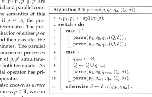
is the set of accepting states.

Algorithm 2.1: parse (p, qo, qa, (Q, 5)) 1 *,P1,P2 +- split(p);

2 switch * do

3 case

+

4

parse(pi, qo, qa, (Q,

5))

_;

5

L

parse(p2,

qo,

qa, (Q, ))

;

6 case '-'

7 qnew +- 0;

8 Q --

Q

U qnew;

9

_{parse(p, qo, qnew, (Q,}

_));

10

L

parse(p2, qnew, qa, (Q, 6)); 11 otherwise J +- 5 U (qo, p, qa);

2.4 DIFFERENTIAL GAMES

A process p is said to evolve to a process p' after actions a1, a2,.. .,an if there is a sequence

of states q1,q2, .. qn+1 in G(p) such that 7r(qi) = p and (qi,ai,qi+1) E 3 for all 1 < i < n

with 7r(qn+1) = p'. We can now define the trace of a process p as a sequence of atomic actions

p = (ai, a2, ... , an) for which the corresponding sequence of states q1, q2,. -., qn+1 exists such that

(qi, ai, qi+1) E 3 for all 1 < i K n. The set of all traces of a term p is denoted by TG(p). Note that

we have modified the conventional definition of the process graph to include the set of accepting states F, which contains nodes without any outgoing edges. The set of traces of p that end at a state inside F are called accepting traces. In this context, let us define a function COStG (q) to be the length of the shortest accepting trace of q. Note that COStG(q) = 0 if q E F. As an example, the process graph for c - (a

+

b)

+

(d + e) shown in Fig. 2.2 has three states with the different traces

being c, c.a, c.b, d, e. All traces except the first one are accepting traces. Given a BPA expression, the product graph G can be constructed using a simple recursive parser as shown below.

Parse Trees for BPA

PA terms (see Def. 2.7) are composed of atomic actions and sub-terms. In Alg. 2.1 we describe a recursive-descent parser that directly builds the process graph (see Def. 2.8) from a given process algebra termp E T by scanning the specification top-down and parsing the sub-terms encoun-tered, while states and transitions of the output process graph are modified accordingly.

The split(p) procedure returns an operator * c {I+, .} and terms p1, P2 E T such that p =

p1 * P2. A process graph for any p E T can then be generated by executing parse (p, qinit, qa, (Q, 3))

where qo, qa are the initial and final states respectively, and Q {qinit, qa} and 3 = 0.

2.4 Differential Games

We now introduce some background in game theory for multi-agent systems that are considered in Chap. 5. Let us first formalize a differential game between two players along with the notion of a Stackelberg equilibrium and then discuss the general n-player Nash equilibrium [B3O95].

In this thesis, we consider games between the robot (R) and multiple-external agents, the dy-namics of all the external agents is clubbed together into a dynamical system which we the "en-vironment" (E). We can thus pose this as a two-player differential game. If X (xr, Xe)T be the combined state of the game, the dynamics can be written as

dx

(X(t),Ur(t), U Ue(t)) = _{,(r(t),Ur(0) (2.2)}

dt

fe(xe(t),

Ue(t))

for all t E R>O where Xr E Xr C Rdr, Ur E 'r C JRmr and Xe E Xe C Rde, Ue E Ue C ERn. The

functions fr : Xr X Ur -+ Xr and fe : Xe x Ue -+ Xe are assumed to be differentiable, measurable

and Lipschitz continuous in both their arguments. Given a trajectory of the game x : [0, T] -+ X, let the corresponding trajectories of R and E be Xr and Xe, respectively.

Stackelberg Equilibria

Consider a game where R and E optimize the cost functions Je (X0, Ur, Ue), Jr (X0, Ur, ue), respectively.

Let the information structure be such that R knows the cost function of E, but E does not know the cost function of R, i.e., it has no information of the intention of R. E however knows the control law

2.4 DIFFERENTIAL GAMES

of player R and can take it into account while devising its strategy. Define BR to be the mapping

from a trajectory ur : [0, T] --+ Ur to ue : [0, T] -+ Ue such that BR(ur) = _{arg min Je(xo,ur,ue).}

Ue

BR(ur) is thus the best response that E can take given a control trajectory of R. The player R then picks its best strategy u* such that

Jr(xou

*,u *) < Jr(xo,u',BR(u')),

where u* = _{BR(u*) for any u'. Such a strategy, i.e., (u*, u*), is called an open-loop Stackelberg}

(OLS) equilibrium for this differential game. Necessary conditions for the existence of open-loop

Stackelberg equilibria can be characterized as shown in [CCJ72J.

Nash Equilibria

Now consider a team of robots, say with indices {1,..., N}. Each robot is modeled as a dynamical system governed by

xi =

fi

(xi(t),ui(t)), xi(0) = xi,init, (2.3)

where xi(t) C Xi C Rdi and ui(t)

E

di C Ri for all t E R;>₀. Given trajectories {x1, x2,. I Xn}

of all agents, where each xk : [0, Tk] - Xk, we require that xks belong to some computable set,

say feasiblek. For example, feasiblek consists of all trajectories of agent k that do not collide with other agents and reach some goal region Xgoal,k. Let JIk (xk, Uk) be the cost function that agent

k would like to minimize; here Uk : [0, Tk] --+ U4 is the control trajectory corresponding to Xk. We can then define the celebrated Nash equilibrium for this problem as follows.

Definition 2.9 (Nash equilibrium). A set of trajectories Y = {x1, x2,. - -, xn

}

is a Nash equilibrium

if for any 1 < k < n it holds that xk is feasible and there is no feasible x such that JIk(x, u,) <

Jk(Xk, Uk ).

The Nash equilibrium is thus a set of strategies such that no agent can improve his cost by unilaterally switching to some other strategy. It can be shown that such an equilibrium is not optimal in the "social" sense. The Pareto optimal equilibrium, on the other hand, is a notion that characterizes the socially optimal behavior.

Definition 2.10 (Social (Pareto) optimum). A set of trajectories Y = {x1, x2,. -, xn

}

is Pareto

opti-mum if all xks are feasible and if there does not exist a set X' = {xf, x/,.. , x

}

such that all x's are feasible and Jk(x', u') <

Jk(xk,

Uk) for all 1 < k < n.

In other words, Pareto optimum is such that no agent can improve its cost without increasing the cost of some other agent, in other words, it is the social optimum if all players cooperate with each other. Necessary conditions for existence of open-loop non-cooperative equilibria, for special cases, e.g., LQR games, can be found in [B095].

CHAPTER

3

Minimum-violation Planning

This chapter discusses the problem of control synthesis for dynamical sys-tems to fulfill a given reachability goal while satisfying a set of temporal specifications. We focus on goals that become feasible only when a sub-set of the specifications are violated and motivate a metric known as the level of unsafety which quantifies this violation, for a trajectory of the continuous dynamical system. We will use ideas from sampling-based motion planning algorithms to incrementally construct Kripke structures.

A product automaton that captures the specifications is then used in

con-junction with the Kripke structure to compute the optimal trajectory that minimizes the level of unsafety.

3.1 Level of Unsafety

Let A be an NFA with some associated natural number, which we call its priority CD (A). We

assume here that the empty trace by convention is always accepted by A. Define the level of unsafety as follows.

Definition 3.1 (Level of unsafety). Given a word over 2H, w = to, f1,..., fn for any index set I = {ii, i2, . , } C {0, 1,...,

n},

define a sub-sequence

W'/ = to, fij-1, fiji1, - - - , 4 ,

where 1 < j < k, i.e., w' is obtained by erasing states from I. The level of unsafety A (w, A) is then defined to be

A(w, A)= min (w) -

(w')

w'EL(A)

where (w) denotes the length of w and L (A) is the language of automaton A. Similarly, define the level of unsafety of a timed word wt(x) = (to, do), (21, d),..., (fn, dn) produced by a trajectory of

a dynamical system to be

A(x, A) = min Ldi v (A). w'EL(A) _iEI

This definition, with a slight abuse of notation thus measures the amount of time wt (x) violates the specification A. For a trace p = so,

... , sn+1 of a durational Kripke structure, it thus becomes

A(p,A) = min T A(si,si+₁) cv(A).

W'EL(A) _iGI

3.2 PROBLEM FORMULATION

of some NFA Aij with priority

cv(Aij).

The ordered set T and cv is then formally defined to be the

set of specifications with priorities. We can now easily extend the definition of level of unsafety

from that of a single automaton to the set of safety rules as shown below.

Definition 3.2 (Level of unsafety for a set of rules). Level of unsafety with respect to a set of specifications 'T and priorities

co

is defined to be

A(w, Ti) = A(w,Ai j) A1ij',i

A(w,) =[A(wjY1),.. .,A(w,Tm)].

A (x, IY) and A (p, ) are defined similarly. A (w, "Y) as defined above is a m-tuple and we use the

lexicographic ordering to compare the level of unsafety of two words.

Thus "Yi for 1 < i < m are m priority classes, each with some number of specifications given using finite automata. Def. 3.2 uses the lexicographic ordering, however as we demonstrate in Chap. 5, we can appropriately normalize A(w, A) and construct a scalar version of A (w, T).

3.2 Problem Formulation

We are now ready to formulate the problem of minimum-violation motion planning. Consider a compact set X E Rd and let xiit E X be the initial state of the system, similarly let Xgoai c X be some compact set called as the goal region. Given the dynamical system in Eqn. (2.1), let us define a task specification to be "traveling from xinit to Xgoai". The finite word produced by a trajectory

x : [0, T] --+ X, w(x) = fo, f1,. .., ,n is said to satisfy the task ( if fo = L,(xinit) and en E Lc

(Xgoai)-Similarly, a trace of the Kripke structure K satisfies the task if the labels of the first and final states of the trace are L,(xinit) and Lc(Xgoai) respectively. We will assume here that this task is always feasible without considering any specifications. The problem that we tackle in this chapter can then be formally described as follows.

Problem 3.3 (Dynamical system form). Given a dynamical system as shown in Eqn. (2.1), a task

spec-ification P, a set of safety rules with priorities (1Y,

cv)

and some continuous, bounded function c(x) which assigns a non-negative real cost to any trajectoryfind a trajectory x* : [0, T] -+ X such that

1. w(x*) satisfies the task specification 4;

2. A (x*, 1Y) is the minimum among all trajectories which satisfy the task;

3. c(x*) is minimized among all trajectories that satisfy 1 and 2 above.

The solution of this problem as defined above exists if the task 1 is feasible. In this work, we restrict ourselves to cost functions c(x) = f6' 1 dt, i.e., minimum-time cost functions. The

algo-rithm in the sequel can be easily modified for other types of cost, e.g., control and state based cost

by appropriate modification of Defs. 2.1 and 3.1. In particular, instead of a "durational" Kripke

structure, we would consider a weighted Kripke structure that also stores the cost of optimal tra-jectory between the two states.

In order to develop an algorithm approach to Prob. 3.3, we convert it into the following prob-lem defined on trace-inclusive durational Kripke structures. We show in Sec. 3.3.3 using Thm. 3.11 that the solutions of these two problems are the same.

3.3 ALGORITHM AND ANALYSIS

Problem 3.4 (Kripke structure form). Given a durational Kripke structure K = (S, sinit, R, I, L, A) that is trace-inclusive with respect to the dynamical system in Eqn.(2.1), a task specification 'D, a set of

safety rules (i, cv),find a finite trace p* = so, si,..., sn such that

1. p* satisfies (D,

2. p* minimizes A(p',f ) among all other traces p' of K that satisfy the task,

3. p* minimizes (p") among all traces p" that satisfy 1 and 2 above.

3.3 Algorithm and Analysis

This section describes an algorithm for finding minimum-constraint violation trajectories for a

dynamical system. We first construct a weighted automaton whose weights are chosen such that the weight of an accepting run equals the level of unsafety of the input word. We then propose an algorithm, based on RRT*, to incrementally construct a product of the Kripke structure and automata representing safety rules. Roughly, the shortest path in the product uniquely maps to a trace of the Kripke structure that minimizes the level of unsafety. Let us note that the algorithm returns a trajectory that satisfies all rules and minimizes the cost function if it is possible to do so.

3.3.1 Weighted Product Automaton

Given an automaton Ai1 E 'T, we first augment it with transitions and weights such that the

result-ing "weighted automaton", Ai, also accepts all words w that do not satisfy Aij, but it gives them a weight. This weight is picked in such a way that the weight of a non-accepting run is exactly equal to the level of unsafety (cf. Def. 3.1). The objective is to combine all Aij into a single weighted automaton ANy that weights its input words according to safety rules 'F with priorities CV. In line with the usual model checking procedure, we then construct the product of the Kripke structure K with Ay. The crucial aspect of this work is that in addition to generating K incrementally using sampling-based methods, we can also construct the weighted product P incrementally.

We now proceed to describe each of these steps in detail and summarize the purpose of each construction in a lemma.

Definition 3.5 (Weighted automaton). For a non-blocking NFA A = (Q, qinit, E, 6, F), the weighted

NFA is defined as A = (Q, qinit, E, 5, F,W) where J = b U { (q,o-, q')

I

q, q' E Q, r

E E

}

and

W(T)=(0 if T E b

cv(A) ifTCE 3\6.

Lemma 3.6. Language of

A

is E* and weight of its shortest accepting run w is equal to A(w, A).

Proof The proof of this lemma follows from Lem. 1 in [THK 13]. U

Definition 3.7 (Automaton A-T). The weighted product automaton A = (Qy, qinit', E, 4, F, Wy)

of automata Aij is defined as

* Q Q1,1 ... X ... Qi,m ... X Qn,- -- X ...

Qnmn;

* qinit,N ~~ (qinit,1,1, - --, qinit,n,mn ;