Approximating optimal state feedback using neural networks

May, 1994 LIDS- P 2249

Research Supported By: NSF grant ECS-9216531

EPRI contract RP8030-10 NSF graduate fellowship

Approximating Optimal State Feedback Using Neural Networks

McDermott, W.E. Athans, M.

May 1994 LIDS-P-2249

Approximating Optimal State

Feedback using Neural Networks *

Wesley McDermott and Michael Athans

Room 35-406

Department of Electrical Engineering and Computer Science

Massachusetts Institute of Technology

Cambridge, MA 02139

33rd CDC

Keywords: Neural networks, Optimal control, Trajectory based data set

Abstract

The training and usage of multilayer neural networks on discontinuous (e.g. bang-bang) feedback control problems are discussed. Training sets are cre-ated from optimal open loop trajectory information and a heuristic for trim-ming the base data set is presented. Apriori knowledge about solution tra-jectories is seen to improve the training process.

1

Introduction

Consider a plant with limitations on the control inputs and a corresponding cost functional to be minimized. Solving for the optimal controls in feedback form, even when given full state information, is not a trivial task. Given an initial state, iterative techniques do exist for calculating the optimal controls via numerical solution of the associated two point boundary value (TPBV) problem [4]. This is an "open loop" trajectory; no knowledge of optimal

*This research was supported in part by an NSF graduate fellowship, in part by NSF

controls for states off this trajectory is obtained. However, it is typically desirable to have a "closed loop" controller that will drive any state in a desired region to the origin, directly mapping measured states into optimal controls.

"Neural networks" have been hailed as a useful tool for approximating an input to output mapping over a closed region of state space [3, 6]. Given a sufficient amount of optimal state space (input) to control (output) informa-tion the neural network can be trained to act as a closed loop controller for a plant. However, effective training of a neural network on a given problem is often a reflection of the researcher's experimentation with various heuristics in a search for rapid convergence to a good solution. The effectiveness of a training technique is ultimately dependent on the combination of network architecture, cost functional, and data set.

Discontinuous (e.g. bang-bang) optimal control problems involve plant, cost functional, and control restrictions that result in controls switching "hard" between a discrete set of values as the plant state moves along a trajectory toward the origin. An explanatory physical example is that of a vehicle on a line to be moved from a given position and velocity to a "stop sign" at position zero as fast as possible. The vehicle is limited in its ability to accelerate and brake. The time optimal control will require accelerating as fast as possible to a certain point and then braking as hard as possible. The extremes of the single control input are in this case the "bang-bang" values of the control.

Consider training a neural network using trajectories obtained from a "black box" that can calculate (in a computationally expensive manner) the open loop solution to two-point boundary value problems for a given plant. The trained neural network will act as an approximation to an optimal closed loop controller in a "real time" situation, possibly involving noise, where the "black box" solver could not. The neural network thus forms a bridge between the available resource and the desire for a controller. The question of interest here is how the particulars of a discontinuous optimal control problem can be used to set up an effective network training technique, and how the trajectory based nature of the training data will affect the training process and results.

network must learn in an "on-line" fashion [8, 10, 5]. By presuming the avail-ability of a "black box" solver, a simpler "off-line" neural network training procedure can be used while studying the implications of trajectory based training.

2

Problem Statement and Notation

This paper investigates the setup of neural network training for full state feed-back control problems with discontinuous optimal controls and the symptoms of trajectory based training that occur in the trained networks. The focus is on the selection of a trajectory based data set and the effects of that selection as opposed to the training process itself.

Two continuous time plant/cost functional combinations are discussed in this paper. These sample problems have known closed loop solutions that provide a reference for the neural network trajectory based results.

2.1

Time/Fuel Optimal Double Integrator

This plant is very similar to the vehicle/stop sign problem described in the introduction, but with a penalty for fuel usage associated with accelerating and braking.

The two state system is defined as [1]:

,xl (t) = x2(t) (1)

x2 (t) = u(t)

where u, the control, is restricted in magnitude:

lu(t)l < 1 (2) x1 represents the position of the vehicle, and x2 represents the velocity of the

vehicle.

The total cost to be minimized is defined as:

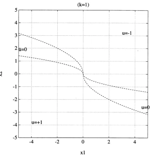
J =~ [k + lu(t)l] dt (3)

where T is defined as the finite time when the state x = 0. In this paper

k=1.

The solution to this problem is derived in [1] and has the form of figure 1. (k=l)

u=-1

-2

-52 _{... ..... .:.. ... ...} - _...

Figure 1: Optimal Switch Curves for the Time/Fuel Double Integrator Prob_{3 -l = -gk--'i'}

0 .... ~ ... ... 4... ' ! ... . ...

k + 4

2k

There are three possible control values -1, 0, +1. An optimal trajectory of a vehicle switches the control a maximum of two times: for example, the vehicle may initially "brake" (u = -1), then coast (u = 0, constant velocity

X= horizontal line in state space), then accelerate (u = +1) to the origin.

2.2

Time Optimal Harmonic Oscillator

This perfectly observed two state plant is to be driven to the origin using two controls in minimum time:

x1(t) = x2(t) + u(t) (5)

xi2(t) = -x1(t) + u 2(t)

J=

dt

(6)

As in the double integrator problem, the controls are individually limited in magnitude; lui(t)l < 1 and lu2(t)l < 1. The solution is derived in [1] and

appears in figure 2.

The state space is divided into four regions, each with a corresponding opti-mal control. Clockwise from the first quadrant the optiopti-mal controls are:

u=[-1,-1], [-1,+1], [+1, +1], [+1,--1] (7) Optimal trajectories consist of clockwise arcs spiraling in to the origin. The example trajectory in figure 2 is the optimal path from x(0) = [3, 3].

2.3

Neural Network Architecture

A standard multilayer neural network will be used, with a single hidden layer combined with an output layer. For a detailed description of multilayer neural networks see [2, 3]. Hidden layer nodes will have a transfer function extending from -1 to +1:

,.

)..

.

...

. Ex. trajectory

/

i\2

.

. ... . . . . ...

...

... ..

[1=+1,

12=+1

-3

.. . . : .

.

.

.

. . . .. . . .. .

Figure 2: Switch Curves and Sample Trajectory for the Time Optimal Har-monic Oscillator Problem

where zli is a scalar input to the node formed from the input state and the network parameter matrix W1 and vector b, (see figure 3):

Zli = [Wlil . * Wlin]X + bzi (9)

n is the length of the input vector x. The vector output of the hidden layer is defined as:

where p is the number of hidden nodes.

The number of hidden nodes is typically determined empirically. In this research the number of hidden nodes varied from thirty to one hundred. Thirty nodes was found to be sufficient to train the networks for both prob-lems; extra nodes slowed training but did not adversely affect the training observations. The examples displayed in this paper were trained using fifty hidden nodes.

The discrete set of control values found in these example problems with dis-continuous solutions indicates that the neural network is actually perform-ing a classification task, formperform-ing a static map between a state and a control "class". As a result, the output layer is chosen to be made up of softmax units, with each unit corresponding to an optimal control value. The network architecture corresponding to the double integrator (three possible control) case is shown in figure 3. Given the weighted input vector to the output layer:

z2 = W2u((WlX + bl) + b2 (11)

the softmax outputs are defined as:

eZ2i

EPr1 ez2r

The softmax unit outputs range from zero to one, and sum to one by defini-tion. When used to control a plant, the softmax units will be implemented in a "winner-take-all" fashion:

1. The current state is input to the network, 2. the softmax outputs are calculated,

3. the control corresponding to the softmax unit with the largest value is applied to the plant.

In figure 3 for example, if for the current state x, ys > ys and ys > y], then the control u = 0 would be applied to the plant.

The network architecture for controlling the harmonic oscillator is the same as in figure 3 except that there are four softmax output units. Each unit

B B bias vector 2 IY (u = ) x 1 ~ x2 Ys Layer 2 Layer 1 nI units

3 Softmax

1 Hidden Layer

Outputs

Figure 3: Network Architecture for the Double Integrator Time/Fuel Con-straint Problem

corresponds to one of the four optimal control vectors from the list in 7 and seen in figure 2.

Given a data set, training the network takes place using the popular gradient descent technique known as incremental backpropagation. Incremental back-propagation involves updating the network weights after each input stimulus is presented. The order of stimulus presentation is reset randomly after each pass through the data set. A momentum parameter can be added which attempts to speed training and avoid local minima. In this work, parameter updates follow the formula from reference [2, chapter 6, equation 6.24]. The learning rate rj during pass t through the training set is defined as 7r(t) = N

where N is the number of training pairs in the data set. The momentum parameter used to speed learning is c = 0.8. For further detail on backprop-agation and its variants, see [7, 9, 2].

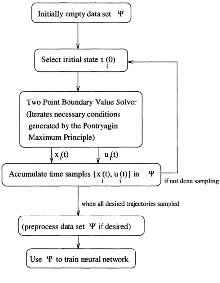
Initially empty data set '

Select initial state x (O)

Two Point Boundary Value Solver (Iterates necessary conditions

generated by the Pontryagin Maximum Principle)

x (t) i uit)

Accumulate time samples { x (t), u (t)) in 'P

i i if not done sampling

when all desired trajectories sampled

(preprocess data set ' if desired)

Use ' to train neural network

3

Development

Given the plant, neural network architecture, and training algorithm, the selection of a data set is the remaining element needed before the network is trained. In the general case the data set will be generated from optimal open loop trajectories via a "black box" two point boundary value (TPBV) solver for a given plant. Figure 4 depicts the general process of creating the data set. In the examples in this paper, prior knowledge of the feedback solution meant that Runge-Kutta integration was used instead of TPBV solvers to obtain trajectory data.

The two main features that will characterize the data set are its distribution, which will result from the choice of initial conditions fed to the trajectory solver, and its size, measured by number of data pairs.

3.1 Distribution of the Data Set

In selecting initial conditions to feed to the trajectory solver and hence to the training algorithm, one has a choice between randomly selecting initial conditions or hand-picking initial conditions in some "suitable" fashion. The underlying presumption is that some limits on the state magnitudes of in-terest are known; i.e. the network is to approximate the optimal control solution well at least within some specified region around the origin.

Random initial conditions, uniformly distributed in some subset of the region of interest, appear the quickest way to begin network training, and assume no special knowledge about the plant and its trajectories.

Selecting the initial conditions purposefully would suggest that some knowl-edge about the state trajectories of the plant is known; perhaps initial con-ditions are selected that are believed representative of the entire state region of interest, or perhaps the controls in some portion of the state space are known to be particularly important to minimizing the cost functional. In other words, initial conditions are being selected because they are a priori believed to improve the effectiveness of the data set in training the neural network quickly and accurately as compared to a random selection.

3.2

Size of the Data Set

A trajectory returned from the two point boundary value solver might well contain a large number of state/control pairs, approximating a continuous trajectory from an initial condition to the origin. A collection of these tra-jectories may contain so many data points that the training algorithm will slow to a crawl. This is particularly true as the number of network nodes increases (recall from section 2.3 that fifty hidden nodes are used in these examples). Thus it would be valuable to examine the information contained in these trajectories and attempt to remove "less necessary" data points in an effort to speed the training process without compromising the quality of the trained network mapping from states to controls.

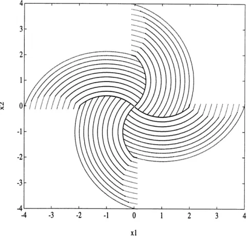
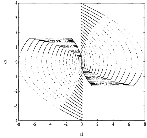
Figures 5 and 6 display a collection of trajectories selected as an example for this research. The forty initial conditions for the double integrator yielded 21612 training pairs (state/control), and the forty initial conditions for the harmonic oscillator yielded 10672 training pairs. As these figures illustrate, optimal trajectories for "classification" control problems consist of several arcs, each with a constant control value. Yet it is the data pairs near the switch curves that provide the critical information about the proper state to control mapping. The data pairs near the center of each arc provide largely redundant information about how the region between two switch curves cor-responds to a constant control value (figure 7).

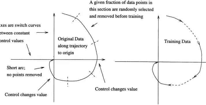
This is not to suggest that the data near the center of each arc is useless. Indeed, removing this data altogether would make good training results in-feasible for two reasons. First, a data set concentrated entirely around the optimal switching curves would result in invalid outputs in the large "be-tween switch curve" regions where there would be no training data. Second, in higher dimensional state cases switch curves can be switch surfaces, and it is valuable to keep information that reflects the position of these surfaces. The heuristic used in this research, labeled trajectory subsampling, is to remove a large percentage of a given central fraction of each arc of constant control. The actual points removed are selected randomly within the central portion of the arc (figure 8). To avoid losing information about small arcs, no data is removed from any arc with fewer than a threshold number of data points.

4

3

2

-xl

-8 -6 -4 -2 0 2 4 6 8

Figure 5: Trajectory Training Data for the Double Integrator Time/Fuel Problem

The heuristic parameters used in this research are:

Double Integrator Harmonic Oscillator

Minimum Arc Size = 100 50

Central Arc Percentage = 70% 85%

Percent to Remove = 90% 95%

A subsampled training set is displayed in figure 9. The trimmed data sets contained 9338 points for the double integrator and 5284 points for the har-monic oscillator.

4r

-4 -3 -2 -1 0 1 2 3 4

xl

Figure 6: Trajectory Training Data for the Harmonic Oscillator Problem

4

Findings

For the double integrator plant, the neural network architecture described in section 2.3 was trained using the regularly spaced initial conditions of figure 5 and separately using a random initial condition data set. This latter set contained forty initial conditions uniformly selected from {x11, Ix21 < 4, and trajectory subsampling was applied.

Similarly networks were trained for the harmonic oscillator problem using the selected initial conditions of figure 6 and from a data set separately formed from forty random initial conditions and trajectory subsampling.

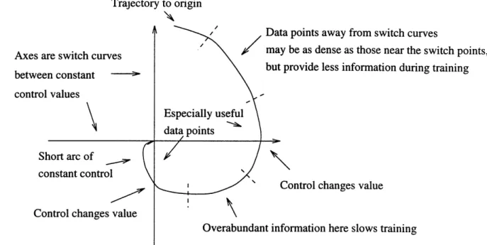
Trajectory to origin

/ i >I Data points away from switch curves

Axes are switch curves ' \ / may be as dense as those near the switch points, between constant but provide less information during training between constant ' control values Especially useful data points " Short arc of / / constant control

Control changes value

Control changes value

Overabundant information here slows training

Figure 7: Data in the Center of Arcs Contributes Little to Training Symptoms of these trajectory based training examples were found both close to the origin, where the trajectories congregate on "terminal arcs" leading to the origin with a constant control, and away from the origin, where im-balances in the training data affected the trained network's switch curves. These observations are discussed in the following sections.

4.1

Data Distribution Away from the Origin

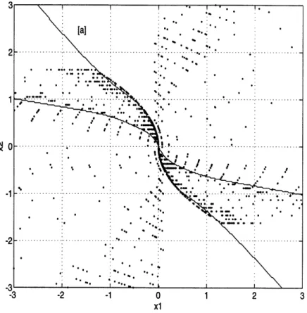
Compare figure 10, the result of training using hand-selected initial condi-tions, with figure 11, the result of training using random initial conditions. In the hand-selected case, the lack of training information above the switch curve in quadrant two results in a roll-off of the network switch curve away from the optimal switch curve (curve [a]). In the random case however, there are training points up in quadrant two, but none defining a switch point. In

A given fraction of data points in this section are randomly selected and removed before training Axes are switch curves

between constant

control values Original Data Training Data

along trajectory \

Short arc; \

no points removed

Control changes value Control changes value

Figure 8: Arc Data Randomly Removed From Center Region

reducing the training error, the network switch curve is pushed away, pinch-ing the u = 0 region undesirably (curve [b]).

Simulation using a network controller with curve roll-off results in the larger initial conditions switching too late to reach the origin in an optimal manner; the trajectories circle the origin an extra time and then are driven properly by the valid switch curves near the origin. Simulating a controller with a pinched

u = 0 region and an initial condition in that region results in controls that

switch repeatedly. The imaginary vehicle brakes then coasts repeatedly as the state works its way along the switch curve until the network and optimal switch curves match near the origin.

These roll-off and pinching effects are caused by the distribution of data present in the trajectory data. These opposing effects point out how a more careful selection of initial conditions could improve a network solution by

4 2 2 -3 -3 -8 -6 -4 -2 0 2 4 6 8 xl

Figure 9: Reduced Trajectory Data for Double Integrator Problem avoiding these extremes. There is clearly a tradeoff between obtaining a base solution in a timely manner or putting in extra time and effort to improve the solution. Unfortunately, in higher dimensional spaces it may be more difficult to see where data should be sampled to improve the training process, increasing the effort required for an improved solution.

The disadvantage of randomly selecting initial conditions is further exempli-fied by figure 12 for the harmonic oscillator problem. Although the initial conditions were selected uniformly over the state space region of interest, the distribution of switch points resulting from these trajectories is clearly not uniform. Compared with figure 2, the quality of the trained network's

switch curve varies significantly. Since relatively few switch curve crossings take place far from the origin, the correspondence between the optimal and trained switch curve is particularly poor near the edge of the region of inter-est.

4.2

Terminal Arcs Near the Origin

Classification control problems will have only a small set of optimal trajecto-ries that lead directly to the origin with a constant control (review figure 1). All optimal trajectories must switch onto one of these paths, or "terminal arcs". As a result, the number of data points along these arcs will accumu-late as trajectories are added to the training set, biasing the network training process to "particularly minimize" the error near these arcs.

In the harmonic oscillator example emphasizing these arcs close to the origin is a desirable effect. This is because the cost of a trajectory in this prob-lem (recall equation 6) turns out to be most dependent on how the state is controlled near the origin. For example, the plant was controlled with the partially trained network with switch curves displayed in figure 13. Notice that at this early point in the training process the network contains little of the optimal switch curve detail. Nonetheless, the extra cost incurred by the non-optimal controller was only approximately five percent for various sample trajectories (from untrained initial conditions).

In the double integrator case however, the accumulated data along terminal arcs tended to "swamp" what little non-terminal arc data points happened to be near the origin. As is visible in the center of figure 11, the switch curves of the trained network do not meet at a point but rather along a short line segment, pinching out the u = 0 optimal control region near the origin. Notice that the pinching effect is more pronounced in this random data case than in figure 10 since fewer random trajectories contained switch

points close to the origin.

While the pinching does not prevent the neural network from successfully controlling the double integrator plant, it appears that the accumulation of data points along the terminal arcs could have been trimmed before training. This could have speeded training slightly without affecting the performance of the trained network. This is a second example link between time spent

preparing the training set and the effectiveness of the training and imple-mentation of the neural network controller.

4.3 Beyond the Training Region

It is desirable for the controller to act "reasonably" beyond the training region, so as to drive the state generally towards the origin instead of away. In both the double integrator and harmonic oscillator examples this was the case. The double integrator switch curves at the edges of figures 10 and 11 continue roughly linearly out beyond the training region. The harmonic oscillator switch curves in figure 12 also extend linearly beyond the training region. This result is sufficient for these examples to drive the state toward the training region, albeit in a non-optimal manner.

5

Conclusion

The selection of the initial conditions used to create a training set have a sig-nificant impact on the performance of the trained network. Prior knowledge of state trajectory behavior is seen to facilitate the selection of a represen-tative set of trajectories that adequately locate switching surfaces. Extra setup time taken to trim the data set will reduce the training time while the features of trajectories from classification control problems can be exploited to avoid losing the most significant training information.

The double integrator and harmonic oscillator control problems permitted the investigation of the symptoms of trajectory based training. In particular, example "reactions" of a standard training algorithm to the nonuniformities in the training distribution were observed. The value of specially trimming the data set, such as to reduce the accumulation of identical trajectory data, is found to vary based on the particular problem, which suggests that clever-ness in approaching a given problem will be rewarded over following a fixed technique for training neural networks.

Figure Sc:h C 1: Te e a c o T e D o. C as ... ... n r ... ... .- . . . . ._. . : ... " . ... ... . ... .3. . ' 2 .3 . ,' 1 . e -3 -.1 .- . .

's ? . ' ... .... . . '. . . ... '. ... .-I. ... ... .. .... ... 1 · ~ 1x~ 1 . 2 -1~T~i~~ _-3 ~ ~ ... ... ... ·... .. , ' .,, i- . .,' :~~~~8--~~~~~~~ · "~~~"~~111-- - - -~-- - - - - --~- ~ ~~~~~~~~~~~~~~~~~~~~~~~~~~~~~~~~. · , .~. < '

3 . 2 . ... . ... . .... ... ... ... CM ... . ... . -2 . . . ... -2 . . . . 'I .NetWork. O m . ... -2 -e oA ... ... pm... .... . ... -4 -3 -2 -1 0 1 2 3 4 xl

Figure 13: Optimal and Partially Trained Switch Curves for the Harmonic Oscillator: Trajectory Costs are Similar

References

[1] M. Athans and P. L. Falb. Optimal Control: An Introduction to the

Theory and its Applications, pages 703-710,595-609. McGraw-Hill Book

Company, 1966.

[2] J. Hertz, A. Krogh, and R. Palmer. Introduction to the Theory of Neural

Computation. Addison-Wesley Publishing, Redwood City, CA, 1991.

[3] K. Hunt, D. Sbarbaro, R. Zbikowski, and P. Gawthrop. Neural networks for control systems - a survey. Automatica, 28(6):1083-1112, 1992. [4] Donald E. Kirk. Optimal Control Theory. Prentice-Hall, Inc., Englewood

Cliffs, NJ, 1970.

[5] S. Mukhopadhyay and K. S. Narendra. Disturbance rejection in nonlin-ear systems using neural networks. Technical Report 9114, Yale Univer-sity, December 1991.

[6] K. Narendra and K. Parthasarathy. Identification and control of dy-namical systems using neural networks. IEEE Transactions on Neural

Networks, pages 4-27, March 1990.

[7] K. Narendra and K. Parthasarathy. Gradient methods for the optimiza-tion of dynamical systems containing neural networks. IEEE

Transac-tions on Neural Networks, pages 252-262, March 1991.

[8] R. Newton and Y. Xu. Neural network control of a space manipulator.

IEEE Control Systems, pages 14-22, December 1993.

[9] A. van Ooyen and B. Nienhuis. Improving the convergence of the back-propagation algorithm. Neural Networks, 5:465-471, 1992.

[10] Paul J. Werbos. Approximate dynamic programming for real-time con-trol and neural modeling. In David White and Donald Sofge, editors,

Handbook of Intelligent Control, pages 493-525. Multiscience Press, New