An Alternative Method of Long Lead-Time Tool Purchases By
Eric W. Partlan
B.A. Accounting, Michigan State University 1996 B.S. Mechanical Engineering, Michigan State University 1996 M.S. Industrial Engineering, Georgia Institute of Technology 2000
Submitted to the Sloan School of Management and the Department of Mechanical Engineering in partial fulfillment of the requirements for the degrees of
Master of Business Administration and Master of Science in Mechanical Engineering
In conjunction with the Leaders for Manufacturing Program at the Massachusetts Institute of Technology
June, 2002
@2002 Massachusetts Institute of Technology. All rights reserved.
Signature of Author
Sloan School of Management and Department of Mechanical Engineering May 10, 2002 Certified by
Dr. Stephen C. Graves Professor, Sloan School of Management Thesis Advisor Certified by _
Dr. Roy E. Welsch Professor, Sloan School of Management Thesis Advisor Certified by
Dr. Kamal Youcef-Toumi Professor, Department of Mechanical Engineering Thesis Advisor Accepted by
I 'Margaret Andrews
Executive Director of the MBA Program Sloan School of Management Accepted by
Dr. Ain A. Sonin MASSACHUSETTS INSTITUTE Chairman, Committee on Graduate Studies
OF TECHNOL OGY Department of Mechanical Engineering
AN ALTERNATIVE METHOD OF LONG LEAD-TIME TOOL PURCHASES
by
Eric W. Partlan
Submitted to the Sloan School of Management and the Department of Mechanical Engineering
In Partial Fulfillment of the Requirements for the Degrees of Master of Business Administration and
Master of Science in Mechanical Engineering
ABSTRACT
The intent of the thesis is to examine the problem of a supplier with a long-lead time product and a buyer that wants the product as soon as possible. The products examined are build-to-order in a rapidly changing industry, so the reduction of the difference between the two times is important. This paper attempts to lay out two primary ways of thinking about this problem, both of which involve real options thinking. The first is the construction of a management decision tree in which there in an upfront payment that is determined by the discounting of the future cash flows based on some discrete
distribution of the outcomes. The second is through the use of the Black-Scholes equation most commonly used in pricing financial options.
The primary motivation for the project is to try and reduce the lead-time that a buyer faces when a company is purchasing a long lead-time product. The microprocessor industry is moving quickly with chip speeds doubling every year to year and a half. This means that it is difficult to forecast the number of tools that will be necessary if the tool has a lead-time that is as long as the actual product cycle. By reducing the lead-time, it may be possible to better time the delivery of the tools to capture the demand as it appears rather than having the tool arrive late, which means missing revenue, or early, which means having unused capacity on hand.
While this thesis will not answer all of the questions regarding options theory as applied to long lead-time tools, the hope is that this work can be used to lay the future for a more intense study of the subject. The process of thinking about these projects as options, having the right at a future point in time to continue with the project or to cancel the project, is important. This line of thinking has the potential to add an immense amount of value to corporate decisions and should not be neglected.
Thesis Advisors:
Stephen C. Graves, Professor, Sloan School of Management Roy E. Welsch, Professor, Sloan School of Management
ACKNOWLEDGEMENTS
The author wishes to think the Intel Corporation for their support of the Leaders for Manufacturing (LFM) Program and their continued support of LFM interns. The projects presented by the Intel Corporation are challenging and, hopefully, Intel will find some value in this paper. Dr. Karl Kempf deserves particular thanks at Intel for helping to lay the foundation for this the project and providing new ideas when I thought that I had hit a dead-end.
The author wishes to acknowledge the Leaders for Manufacturing Program for its support of this work. Steve Graves, Roy Welsch, and Kamal Youcef-Toumi provided support throughout the project. Without their ideas and feedback this paper could not have been completed. I would also like to thank the friends that I have made while in the LFM program. My classmates have been, and will continue to be, a source of inspiration.
The MIT community, in and out of Cambridge, was helpful in the project as well. Dr. Craig Kirkwood, a business school faculty member at Arizona State University and an MIT graduate, provided direction on the construction of the model and was willing to take time out to review the model as it was in construction. I would also like to thank Dr. Gordon Kaufman from MIT for providing feedback and advice on some of the theory.
I would like to thank my family: Sandy, Charles, and Kris Partlan. Without their support over the past 28 years, through the good times and the bad, I most certainly would not have made it through. Thank you.
TABLE OF CONTENTS
ABSTRA C T ... 3
AC K N O W LEDG EM ENTS ... 4
TA BLE O F C O N TENTS ... 5
TA BL E O F FIG UR ES ... 7
1 INTRODUCTION AND OVERVIEW ... 9
1.1 INTRODUCTION ... 9 1.2 O VERVIEW ... 11 2 PR O BLEM D ESCRIPTIO N ... 12 2.1 BACKGROUND ... 12 3 W H A T A RE O PTIO N S? ... 16 3.1 W HAT IS AN O PTION ... 16
3.2 THE B INARY TREE ... 18
3.3 THE B LACK-SCHOLES M ETHOD... 21
3.4 REAL O PTIONS... 23
3.5 TYPES OF REAL OPTIONS ... 29
3.5.1 The Option to Grow ... 29
3.5.2 The Option to Expand ... 30
3.5.3 The Option to Abandon... 30
3.5.4 The Option to Contract ... 31
3.5.5 The Option to Switch... 31
3.5.6 The Option to Wait... 32
3.6 W HEN ARE REAL O PTIONS VALUABLE ... 33
3.7 PROJECT FIT... 35
4 D EC ISIO N TREE M O D EL... 38
4.1 THE FULL M ODEL ... 38
4.1.1 Real-Tim e Flow ... 44
4.1.2 D ata Flow ... 47
4.1.3 D ata Flow D escription ... 50
4.2 M ODEL D ESCRIPTION... 52
4.2.1 Fixed and Calculated Variables ... 52
4.2.2 D ecision Variables... 62
4.2.3 Uncertainties... 69
4.3 SUPPLIER M ODEL ... 72
4.3.1 Fixed and Calculated Variables ... 74
5 RESULTS AND DISCUSSION ... 80
5.1 STEADY DEMAND SCENARIO ... 82
5.2 ONE-PERIOD DEMAND DROP SCENARIO ... 89
5.3 ONE PERIOD SHARP DEMAND DROP SCENARIO ... 92
5.4 LARGE DEMAND DROP SCENARIO ... 95
5.5 VOLATILE DEMAND SCENARIO... 100
5.6 VOLATILITY WITH A NON-VOLATILE LONG LEAD-TIME FORECAST ... 103
5.7 SUM M A RY ... 106
5.8 BLACK-SCHOLES DISCUSSION ... 109
5.8.1 Working with Black-Scholes ... 115
6 CONCLUSION AND AREAS OF FUTURE RESEARCH... 121
6.1 SU M M A RY ... 12 1 6.2 FUTURE W O RK ... 127
6.3 C ON CLU SIO N ... 130
7 LITERATURE REVIEW AND BIBLIOGRAPHY ... 132
TABLE OF FIGURES
Figure 1. Time Flow... 12
Figure 2. Tool Use... 14
Figure 3. Call Option Payoff... 17
Figure 4. Put Option Payoff ... 17
Figure 5. Stock and Option Prices in a Binary Tree... 19
Figure 6. Range of Future Values ... 26
Figure 7. Range of Future Values and the Distribution ... 27
Figure 8. Uncertainty and Value ... 27
Figure 9. The Value of Uncertainty and Flexibility ... 28
Figure 10. Cone of Uncertainty ... 35
Figure 11. Full Decision Tree... 40
Figure 12. Critical Times... 41
Figure 13. The Decision Tree for the Six-Month Time Frame ... 42
Figure 14. The Decision Tree for the Nine-Month Time Frame... 43
Figure 15. The Decision Tree for the 18-Month Time Frame... 44
Figure 16. Real-Time ... 45
Figure 17. Ongoing Real-Time ... 46
Figure 18. Time Flow of the Decision Tree ... 49
Figure 19. Uncertainty and Decision Flow ... 50
Figure 20. Data Flow in the M odel ... 51
Figure 21. Tool Uncertainty ... 53
Figure 23. Figure 24. Figure 25. Figure 26. Figure 27. Figure 28. Figure 29. Figure 30. Figure 31. Figure 32. Figure 33. Figure 34. Figure 35. Figure 36. Figure 37. Figure 38. Figure 39. Figure 40. Figure 41. Figure 42. Figure 43. Figure 44. Figure 45. Pay-To-Delay... 64
N ine-M onth Exercise... 65
Option Purchase ... 66
Eighteen M onth Exercise ... 68
Tool Uncertainty ... 69
Six-M onth Dem and Forecast ... 70
N ine-M onth Dem and Forecast... 71
Eighteen-M onth Dem and Forecast ... 72
Supplier Decision Overview ... 73
Overall Supplier M odel... 74
Pay-to-Delay on the Supplier Side... 77
Option Exercise on the Supplier Side ... 78
Orders M anufactured ... 79
Dem and for the Steady D em and Scenario ... 83
Cost Comparison for the Steady Demand Scenario... 88
Dem and for the Slight Dem and Drop ... 90
Dem and for the Sharp Dem and Drop ... 93
Dem and for the Large D em and Drop ... 96
Dem and for the Volatile D emand ... 101
Dem and for the Realistic Volatile Forecast ... 104
Tim e Fram e for the Black-Scholes Exam ple ... 115
Option Value and Expected Value... 118
INTRODUCTION AND OVERVIEW
1.1 INTRODUCTION
The purpose of any firm is to create value for the stakeholders and the decisions made by management in any entity should be made in recognition of that. Business managers are now faced with need to make decisions at a more rapid pace than at any time in the past. These decisions have consequences that can ripple through the supply chain with surprising speed and ferocity. The semiconductor industry is, in particular, faced with the need to make quick decisions due to shortened product life-cycles, increasing competition, and hazy demand forecasts.
This project was conducted at the Intel Corporation in Chandler, Arizona with the purpose of examining ways to reduce the lead-time of tools used in the semiconductor manufacturing process. However, the methods discussed in this paper can be used for a variety of purchased products. One can simply change the time frame and the values that were utilized if other products are being examined.
Intel has had the ability to make exceptional profits for most of its history for two reasons. The first reason is the amount of research and development that the company conducts. The company has always felt it was important to invest in the next generation of products. In fact, Gordon Moore predicted that the processing power of
semiconductors would double approximately every 18 months. This law, for the most part, has held true in the industry. For each generation of chip that Intel produced, a
significant portion of the profits were reinvested in developing the next generation of I
chips. This allowed Intel to introduce next generation processors faster than any other company on the market, allowing market domination and high profit levels.
The second reason is the excellence of their manufacturing function. Intel is able to quickly ramp-up production of a new project and bring the price of the product down to a reasonable level. The demand for their products usually skyrockets soon after
introduction while, at the same time, the company is faced with a product life cycle that lasts no more than 18 months. For this reason, the company needs a massive amount of capacity to quickly produce their product and meet their demand. They copy their manufacturing exactly from one site to the next to help make sure that they have the necessary capacity in place.
Through this combination of large investments in research and manufacturing, the company has come to dominate the semiconductor market. However, this domination has led the company to be lax in a number of important areas. The most important to this project is their supply chain design. Up until the mid 1990's, Intel was able to tell each user of their product exactly how much of their demand they would actually receive. For example, Intel may have been able to produce one million chips in a given time period, while demand was 1.2 Million chips. Intel could tell the computer manufacturers that they would only be getting 83% of their requested demand and the computer
manufacturers would have to live within this limit. This allowed Intel to concentrate on manufacturing while leaving their supply chain to be examined later because it just did not matter. If production was delayed for some reason, the product delivery was pushed out and there were no negative repercussions to Intel.
In the mid-1990's, greater competition for Intel started to emerge. All of a sudden there were other companies entering the market (AMD, 3rd party manufacturers, etc.) that
were able to compete with Intel. No longer could Intel tell a manufacturer that they would only receive 83% of their demand. The manufacturers now had other suppliers that they purchase chips from if Intel could not meet the necessary demand. Intel's supply chain became significantly more important as their competitors started to eat away at their market share. It was no longer a non-issue if a tool was not delivered when promised. It meant that Intel had missed out on a significant portion of demand, revenue, and profit. More importantly, Intel could begin to lose customers, as they could not meet supply. Intel's competitors were able to take a small portion of demand, reinvest the profit, and slowly build their capacity until there was viable competition to Intel's domination of the market.
1.2 OVERVIEW
This thesis will begin with an overview and background of the problem in Section 2. Section 3 introduces real options and the current state of real options literature and applications. Section 4 will show a management decision tree model that was created and the variables and formulas in that tree. Section 5 will discuss the results of a number of these scenarios including the shortcomings of the method. In addition, several other potential areas of option pricing are examined. This section will discuss when it makes sense, and when it does not, to examine alternative purchasing arrangements. Section 6 is a conclusion with some potential future areas of research. Section 7 includes an annotated bibliography of papers that the reader may find of interest.
PROBLEM DESCRIPTION
2.1 BACKGROUND
This project was defined as looking at ways to decrease the time on long lead-time equipment purchases. The ultimate goal of the project was to examine ways in which we could decrease time between placing the order for a photolithography tool and receiving the tool. A photolithography tool has amongst the longest lead-time of any tool
in a fabrication facility, with a time of nearly 18 months. It is important to note that a new generation of photolithography equipment is necessary for each new generation of processor. Given that the typical life-cycle for a generation of semi-conductor chips is
18-months, it is apparent that as soon as a new chip is introduced, orders must be placed for the next generation of equipment to produce the next generation of chips. Figure 1 shows the problem that was being examined.
Supplier warts the Buyer wants to place D elivery of
or der pl&ca d hea. the order here. The To
D elta Tim e
TIME Normal equipment manufacturing lead time
Figure 1. Time Flow
The supplier wants the order placed as early as possible for a number of reasons. They need to plan for their headcount, their material flows, and their production space.
The sooner a firm order is place, the sooner the supplier can begin to plan for the manufacturing. At the other end, the buyer of the tool wants to place the order as late as possible. The primary reason for this is because as time goes forward, the buyer has better visibility as to what the realized demand will be. If the order is placed 18-months before the demand will be realized, it is difficult to forecast what the actual demand will
be. If the tool can be ordered nine-months before the demand is realized, the demand
visibility is not as cloudy. The solution has been to order more tools than are actually necessary. These tools cost nearly SlO Million each, so buying excess tools can quickly eat into a company's profit. Figure 2 gives a second view of the problem that was being examined. The x-axis represents time in Figure 2 while the y-direction is representing demand. The demand can be assumed to follow a normal distribution in which demand ramps-up, reaches a peak, and ramps-down. Each of the early tools (tool 1, 2, .... ,n) are tools that will be used throughout the production of the semiconductor generation. The tool capacity that is necessary at the lower level of demand is easy to forecast as this capacity will almost certainly need to be utilized. However, the tools that will be used as demand reaches a peak are much more difficult to forecast. These tools will have a
limited life in that they will be producing product for a short period of time. The tools are brought on-line as the production begins to peak and can be called spike demand tools.
Since these tools are used for such a short period of time, there overall value is reduced as compared to other tools as not as much product will flow through these spike tools. However, to meet demand and ensure profits, they are still necessary.
Tool n+1
Tool1 n -Tool 1
TIME
Figure 2. Tool UseThe demand is not known but an attempt can be made to forecast the demand. Demand is assumed to follow a somewhat normal distribution, so tools 1 through n can be ordered to cover some certain percentage of the demand that we is sure to be realized in extreme downturns. For example, a company may be 100% confident that 50 Million chips in a particular generation will be sold. Therefore, enough tools can be ordered 18-months from the needed date to produce those 50 Million chips. However, the company may think that demand can range up to 80 Million chips even though the expected demand is 70 Million chips. So the expected possible demand on the upside is 80 Million chips, with some uncertainty, while the lowest demand forecast possible is 50 Million chips. The questions is how can the company minimize their exposure to paying for tools that they might not be able to use. That was the central point of the project.
The expectations for the internship were three-fold. The first was to examine ways in which purchasing agreements could be constructed to minimize the overexposure of Intel to excess tool purchases. Different methods of doing this were examined and narrowed down. The second expectation was to examine the method chosen with regards
to what had already been done in the real world. If the project had already been completed then there was no reason to reinvent the wheel. The third purpose of the project was to attempt to build a model that could eventually be used in Intel to assist with purchasing. It was known going into the internship that there was not enough time to complete a fully functioning model that could be used by Intel. However, the purpose was to start a model that could be handed over to Intel for eventual integration in purchasing.
3
WHAT ARE OPTIONS?3.1 WHAT IS AN OPTION
An option is the right, but not the obligation, to take some action in future. An option is valuable when there is uncertainty in the final distribution of the value of the asset. As uncertainty increases, the value of an option increases. The central tenant of options theory is that there is a probability distribution for the final price of an asset. There is an expected value but there is a chance that the value will be higher and there is a chance that the value will be lower. This distribution is characterized by the expected return and the variance of those returns.
There are two basic types of options. The first is a call option. This gives the holder of the option the right to buy the underlying asset by a specified date at a specified price. The specified date of the contract is known as the time-to-maturity and the specified price is called the strike price. An American call option gives the owner the right to exercise the option at any time up to and including the expiration date. A European call option allows the owner to exercise the option only at the date of expiration. In the case of a call option, the owner believes that the value of the underlying asset will increase with time. Upon exercise, the owner can buy the asset at the lower price and sell it at the higher price. Figure 3 shows the payoff on a typical call option.
Strike Price Profit 0 T erminal Loss Asset Price ($)
Figure 3. Call Option Payoff
A put option gives the owner the right to sell the asset by a specified time at a
specified price. In this case, the owner believes that the price of the asset will decrease. This will give the owner the right to buy the asset at the lower price and sell it at the higher price. Figure 4 shows the payoff for a typical put option.
Profit
0
Terminal
Loss Asset
Price ($)
Figure 4. Put Option Payoff
Notice that in the payoff for both the call and the put options, there is a portion of the payoff that has a negative value. This is because the purchaser of an option is required to pay a set price to purchase the option. This is the option purchase price. As Figure 3
shows, before the asset hits the dictated strike price there is a loss of the amount of the premium. If the premium for a call option is $3 with a strike price of $10 and the asset never crosses the $10 value, the holder of the option has lost the $3. When the strike price is hit, the holder begins to make money with the increase in price. When the asset is worth the strike price plus the premium the holder makes money. This is where the line begins to cross the x-axis in Figure 3. Similarly, the owner of a put option will not make money until the price of the asset has dropped below the total strike price less the purchase price of the option.
An investor in an option can take advantage of the upside of a transaction while avoiding the downside. The payoff is truncated in that the downside of the asset movement is cut off while the upside is not. Due to this truncation, it was difficult for people to determine what the proper price to charge for an option. However, academics developed a means of duplicating the cash flows from an option investment by building a basket of publicly traded financial instruments. When this basket can be built, the option price can be determined exactly. This led to three primary means of valuing an option. They are the Black-Scholes method, the binary tree method, and through Monte Carlo simulation. While there are a number of alternative methods, these are the three most used in practice.
3.2 THE BINARY TREE
Consider a stock with an initial value of So, and a single option on that stock with a current price of V (Hull, 2000: The reader is encouraged to examine this reference for a more detailed description of binary tree option pricing). The option has a time to
Sod where u is greater than 1 and d is less than 1. The proportional increase when there is
an up movement in the stock is u-1 and the proportional decrease when there is a down movement in the stock is 1 -d. If the stock moves to the up position then the option has a
value of V, and if the stock moves to the down position the option has a value of Vd. This situation is shown in the following Figure 5.
Su Vu So VV Sd Vd
Figure 5. Stock and Option Prices in a Binary Tree
A fairly simple assumption can be made in pricing the option that only relies on the
principle of no arbitrage, or the law of one price. A portfolio of the stock and option can be set up in such a way that there is no uncertainty about the value of the portfolio at the end of the three months. Since the value of such a portfolio is known, there is no risk and it must earn the risk-free rate of interest.
Imagine a portfolio that consists of A shares of the asset and that is short one option. The value of A that makes the portfolio risk-free can then be calculated. If the asset moves up in value, the value of the portfolio at the end of the life of the option will be SouA - V. If there is a down movement in the stock then the value becomes SodA - Vd.
SouA -Vu = SOdA - V
Or:
Slu - Sod
If the risk free rate of interest is r, then the present value of the portfolio is:
(SouA- Vu)e-T
Note that the exponent is used to recognize that the interest is continually compounded. It then follows that
(SouA-Vu,)e-T = SA-V
This last statement is saying that the cost to set-up the portfolio is equal to the present value given the law of one price. So:
V = SoA- (SuA- V0)e-rT
Substituting the equation for delta and simplifying the equation yields: V=-rT[p V+(l-p)V]
where:
rT d u-d
These last two equations allow an option to be priced using a one step binomial model. This means looking out one period of time in the future and calculating the value of the option at time zero. For example, consider a stock currently priced at $20. The stock will be either $22 or $18 in three months. We would like to value a European call option that expires in three months with a strike price of $21. If the stock ends up worth $22, the option will have a value of $1. If the stock ends up at $18, then the option will
The value for u is 1.1 as $22/$20 = 1.1. The value for d is .9 as $18/$20 = .9. If the
risk-free interest rate is 12% per year, then the value for p andfis
e12*.25 9
P = = .6523
V= e~ 12*.25[6523*1 + (1 - .6523)0]= .633
In the absence of arbitrage opportunities, the current value of the option is $.633. Although binomial trees are used in practice, using a one-step binomial tree is an
extremely simplistic approach. The life of a stock option is usually broken into n time steps of At which leads to 2" possible stock paths. So if an option expires in 30 days and each day is considered a time step, there are 230 possible final stock values. Typically, the up and down movements are chosen to represent the volatility of the stock. That is done by setting:
u =e and d =e
where G is the volatility of the asset and t is the time to expiration, or the time-frame
being examined. These values can be used instead of the set end values of the stock. If one knows the upward and downward movements of the stock then the value for the volatility (sigma) can be estimated. This relationship will be used later in the paper.
3.3 THE BLACK-SCHOLES METHOD
A second method of option valuation is the Black-Scholes Method. The equation
that was derived is a closed form solution for a European option. This is a continuous time domain as compared to binary trees that work in discrete time. For the binary trees, a value has to be assigned at the end of each branch of the tree and then the preceding value of the option is calculated. Imagine breaking the time down into infinitely small
buckets and one can see how this would collapse into a differential equation. There are a number of assumptions used in this equation which are detailed in the bibliography (Black, 1973).
Various equations have been derived that work around one or more of these constraints. For example, there is an equation for valuing stock options that allows for dividends to be paid on stocks, as long as they are predictable. It is also possible to have
a as a function of t or interest rates can be allowed to be stochastic. However, there are
no equations that can work around all of the assumptions at once. Again, in the bibliography, there are sources listed that detail a work around for each assumption (Black, 1989).
The equation for pricing a European call option is shown below.
C, SoN(d)- Xe~rN(d,) where: In(SL) + (r + d1 X 2 and: d2 =d,- at
The variables are:
So= The current price of the stock X = The exercise price of the stock
r = The continuously compounded risk-free interest rate per annum
c= Measure of uncertainty of the returns (volatility = standard deviation of the stock price)
N( ) = Cumulative probability distribution function for a standard normal variable An excellent way to think about the breakdown of the overall formula is:
SON(d) = The expected value of S0 if S0 is greater than X at expiration. The expectations
are taken using risk-neutral probabilities.
Xe-r = Present Value of the cost of the investment.
N(d,) = The risk-neutral probability of S, being greater than X at expiration.
These values can all transfer to the domain of real options. So becomes the present value of all of the future cashflows that are expected from an investment opportunity. X is the present value of the cost associated with the investment opportunity. The volatility is the standard deviation of the growth rate of the future cashflows associated with the asset. The time to expiration becomes the period for which the investment opportunity is valid. This can be the length of a lease or a product life cycle. The risk-free rate of interest remains the same.
3.4 REAL OPTIONS
Real options are a means of looking at decisions, strategic and financial, that take into account ideas that a normal valuation or decision-making process would not. In particular, real options recognize that options are contingent decisions. They give a person the opportunity to make a decision after the events have unfolded. If events have turned out well on the decision day, then one decision can be made. If they have not, then another decision is made. This process allows one to make an attempt to reduce the
Aristotle (Copeland, 1998) writes of how Thales the Melesian, a philosopher, divined from tea leaves that in six-months there would be an excellent olive harvest. Thales spoke with the owners of the olive presses and told them that he would give them money today to be given the right to use the presses in six-months time. In-six months time there was a bumper harvest and the olive growers were in need of all available capacity to press their harvest. Thales rented the presses to the olive growers at a high rate, paid the predetermined rate to the press owners, and kept the rest. He had paid a small fee up front for the right, but not the obligation, to use the olive presses in the future. This is an example of a real option.
In options theory, the predetermined rate that is paid upon exercise is called the exercise price. When the exercise price is lower than the market price, the option is called "in the money". When the exercise price is higher than the market price, the option is called "out of the money. When the olive harvest came about. Thales had an exercise price of the normal cost of using the press while the market price was higher. So his option was in the money.
The value of the option increases with an increase in uncertainty. Imagine the situation where the size of the harvest is known exactly six-months in advance. The owners of the press are then able to plan their capacity precisely meaning that the price charged for the use of the presses will also be normal. If this occurs, then the option that is held by Thales is worthless. However, as the uncertainty increases, the chance that the option will finish somewhere other than the expected value increases. Therefore, the value of the option increases. The source of uncertainty in this story is the size of the olive harvest. This affected the value of the olive presses. As the size of the harvest
increased, there was less excess capacity so the value of press time increased. As the value of the underlying asset increases, so does the option value.
In addition, the time to expiration of the option also affects the value. If Thales had signed a contract with the press owners one-day before the expiration of the option then there would have been very little chance that the harvest would change by a great amount over that one day. However, if the contract had been signed one-year before the harvest, the value would have been larger. This is because the uncertainty has a greater effect as time increases. As the time increases, the chance that the value of the underlying asset
will move up increases, driving an increase in the value of the option.
With this example, the major sources of value in an option are shown. They are the value of the underlying asset, the uncertainty in the option, the exercise price of the option, and the time to expiration of the option. The final variable is the risk-free interest rate. As the interest rate increases, the value of the option decreases because the future cash flows have to be discounted at a higher rate.
Real options are often difficult to recognize when managers are making decisions. Consider the example of life insurance companies in the 1960s that were trying to sign people up for whole life policies. A feature that was often included in the policies was the right of the policy holder to borrow money against the cash value of the policy at a certain fixed interest rate. The interest rates at the time were low, 3% or 4%, so the companies did not think that this feature was important. However, in the late 1970's and early 1980's, interest rates jumped in the double digits. All of a sudden the policy holders were able to borrow against their policies at 8% and the insurance companies had to borrow at a much higher rate to finance their policy holders loans. The life insurance
companies were giving away a call option on borrowing money and not charging a premium. While the life insurance companies almost certainly prices these policies with a normal discounted cash flow analysis, the companies did not take into account the volatility of interest rates.
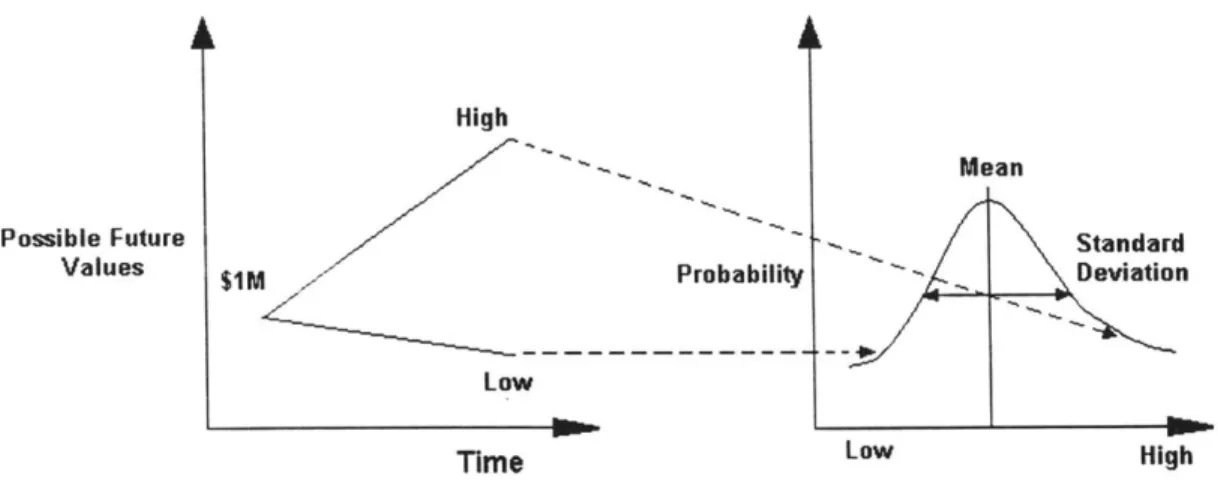
Real options involve uncertainty about two separate items. The first is the future and the other is the ability of management to respond to what it learns as that future becomes clearer. That is the primary way to think about real options. Figure 6 shows an asset or project with a present value of $1 M.
High
Range of
Possible Future i Possible
Values $ Future
$ Values
Low Time
Figure 6. Range of Future Values
As shown in Figures 6 and 7 (Amram, 1998), that project has some future range of values, although it is not known with certainty. The distribution is typically skewed so that the range of positive outcomes is larger than the range of negative outcomes as we expect, on the average, that companies will increase value over time instead of destroy value.
High $IM / Probability Low Time Mean Standard Deviation Low High
Figure 7. Range of Future Values and the Distribution
A company needs to take that uncertainty and try to take advantage of it. In other
words, increase the range of positive outcomes, while trying to reduce the possibility of negative outcomes. In options terminology, purchase a call to take advantage of movement up and purchase a put to protect against any movement down. Figure 8 (Amram, 1998) attempts to show this rotation through the company's assets.
Uncertainty for External Factors Firm's Assets Flexible Investment Strategy Modifies Exposure
Uncertainty for the Value of Strategic Investment
Uncertainty and Value
Possible Future Values
Options are most valuable when there is a large amount of uncertainty in the future and when management has the flexibility to take advantage of the uncertainty. When it is likely that more information about the demand will be received over time, the value increases. This is shown in Figure 9 (Copeland, 1998).
Uncertainty Likelihood of receiving new information Low High Room for managerial High flexiblity Ability to Respond Low
Flexbility value is greatest when:
1. There is high uncertainty about the future and it is likely that new information will be re c eive d over time.
2. There is room for managerial flexibility which gives management the chance to respond.
3. The Net Present Value without considering flexibility is near zero, meanig that
the project is not obviously good or obviously bad so management might want to change direction while the project is in work.
Figure 9. The Value of Uncertainty and Flexibility
It is important to recognize the difference between an option and a bet. Imagine that a company is building a factory for SIM dollars that must be paid entirely up front. If the company does not know what the final demand will be, then this is a bet. The company must either invest the money or not invest the money. Now imagine that this company can go ahead with a $100,000 pilot project and then spend $l.1M in one-years time. They are using the pilot project to see if all will go according to plan or not. If it does,
Moderate High Flexibility Flexibility Value Value Low Moderate Flexibility Flexibility Value Value
$100,000, the company has saved itself SIM in present value terms (assuming a 10%
interest rate). The company has given itself the option to expand. If the project is successful, then the company will have spent $100,000 more than they otherwise would have. However, some managers would think it well worthwhile to spend a little bit more money to garner the information that will help adjust the probability of outcomes favorably.
3.5 TYPES OF REAL OPTIONS
There are a variety of types of real options but, for the most part, they can be classified as one of the following six types of options.
3.5.1 The Option to Grow
The first type of option is the option to grow. The option to grow usually has the greatest potential value in investment decisions. When a company invests in its infrastructure, its people, or its technological base it is buying a growth option. The company now has the ability to make future choices that it was not previously able to make. Research and Development projects are an example of purchasing an option to grow. If the projects are successful then the company has the potential to open a whole new market. If a company invests small amounts of money in 100 different R&D projects to see which projects have early signs of success, they can then exercise their options on the successful pilots.
3.5.2 The Option to Expand
Closely tied to the growth option is the option to expand. In a manufacturing facility, this option might take the form of purchasing a machine that has a negative net present value but sets the stage for future expansion. For example, a firm may purchase a new machine that generates $300,000 of revenue per year but costs $400,000 per year to operate. If they do not purchase the machine now then they are not allowed to purchase the machine in the future. However, in another year a new type of material may, or may not, be developed which will cause this machine to generate $500,000 of revenue per year instead of $300,000. The paper company has purchased a call option that will allow them to expand into this new product. It is important to note that the option for growth and the option to expand are similar in nature.
3.5.3 The Option to Abandon
When a project commences, the company still may have the ability to cancel a project and receive an inflow of cash in exchange. This can be thought of as the salvage value of a project. For example, a real estate company may begin construction of an office building at a cost of $100 Million. The real estate company has a contract from a client to rent the building for $120 Million (in present value terms) over the life of the building. At some future date, during construction, that client has to back out of the agreement for some reason. The real estate company is able to find a new renter but they are only willing to pay $90 Million over the life of the building. If the company can terminate the construction project and sell the partially completed building to another company with a loss of less than $10 Million, the real estate company should do it. This is considered an option to abandon.
This option is equivalent to an American put option. The company can exercise this option whenever they want, which means stopping the construction, and the option allows them to protect against downside risk.
3.5.4 The Option to Contract
Closely tied to the option to abandon is the option to contract. This allows a company to change the scope of the project while the project is in process. For example, a manufacturing firm is building a new factory that has several financial milestones. The company is planning a factory that can produce 10,000 boats and it will cost $5 Million per year over the next five years to construct the factory. If in year two the company decides that they want to scale down the factory so that it only produces 5,000 boats, they will pay only $3 Million. The company has an option to contract because they can decrease the scale of their project. As with the option to abandon, the company has a put option to protect against a sudden decrease in demand.
Like the option to grow and the option to expand, the option to abandon and the option to contract are very similar. Again, they are on the same continuum but at different extremes. The option to abandon is, usually, considerably more valuable than the option to contract because the scope is typically much larger.
3.5.5 The Option to Switch
A fifth type of option is known as the option to switch. This option usually refers to
the ability to accommodate different inputs or different outputs. For example, a manufacturing company is deciding whether to install new furnaces for a new production line that will run off of natural gas, off of electricity, or off of both. The natural gas
furnaces cost $1 per furnace, the electrical furnaces are $1.25 each, and the dual furnaces are $1.5 each. Each type of furnace has the same capacity and produces 1 unit per $ of energy input. Currently, the cost to run the electrical furnace is half the cost to run the natural gas furnace.
In the current state, the company will choose to install the electrical furnaces because the cost of using the furnace is less than the other two furnaces. However, the inputs to these furnaces are volatile and it is possible that in the future the cost of electricity will skyrocket while the cost of natural gas stays the same. If this happens, the company will not be able to produce products at a reasonable price. If the company purchases the furnaces that run off of both inputs, they can switch back and forth depending on which input is less expensive. This is an example of the option to switch. Typically, the less correlated the inputs, or outputs depending on the option, the more valuable the option will be.
3.5.6 The Option to Wait
Every investment decision involves an option to wait. Common sense says that the longer a company or an individual waits to make a decision, the more information there will be available to make that decision with. The emergence of information over time effects an investment and the decision that will be made. There is, however, a trade-off to the waiting in most situations. The company runs the risk of missing out on some of the return from the investment by not investing up front. This is the case when companies do not have monopoly power and face competition.
There are situations where this option has value. For example, a orchard may own land that produces apples on the outskirts of a city that has a quickly developing
technology industry. The company can develop this land for $2 Million and sell it for $2.2 Million. The project currently has a positive net present value but, at the same time, the company recognizes that the real estate market is volatile and that the technology industry is volatile. Even though the net present value is positive, the company may calculate that there is addition value added by waiting a year to see if the real estate and technology industries are going to hold up and continue to grow. The company has a valuable option to wait because the information that they will gather over the next year
may be worth more than the present value of the project.
A second example might take the form of a sleeping patent. A sleeping patent is a
patent on a product or a process that a company holds but is not currently using. For example, an electronics processor may hold a sleeping patent on a new type of digital recording device that it is not producing. The company is not sure how large the market is for the product and is not willing to invest in the capacity to produce the product without knowing. The company can wait for competitors to introduce similar products that define the market size. The company can then begin production of its superior product and steal market share from its competitors. The company gained value by being able to wait to begin production of its product.
3.6
WHEN ARE REAL OPTIONS VALUABLEReal Options thinking is not always a necessity. There are some decisions that require very little in the way of financial analysis and are certain to generate a profit no matter the outcome. In the oil industry, if there is excess demand of two-million barrels per day at $40/barrel (with the price expected to be constant for a certain time period) and we can produce oil at $1 0/barrel, it is obviously advantageous to start producing extra oil.
On the other hand, there are times when options are not necessary because there is no value added from a certain decision. An example of this would be where the price of oil is $10/barrel and we can produce it at $40/barrel. The decision to produce would be incorrect.
Thinking about options is most advantageous when these decisions are in a gray area. The areas where a more traditional net present value decision is hovering around $0 or the times when there are strategic reasons for making an investment. Traditional tools work very well when there are no options to consider in a decision or where there is little uncertainty within a decision. An excellent example of this is the company that consistently generates a specified cash flow that is declining over the years. This company will not have any follow on opportunities and is more than likely in the declining phase of the company or product life-cycle. A company that supplies a certain piece of equipment for a product that is being phased out might be an example of this. This type of company is known as a "cash-cow".
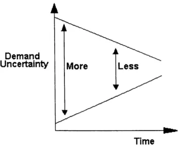
So real options are needed in situations where there is enough uncertainty that is sensible to wait for more information. The goal is to avoid the regret of making irreversible investments that could harm the value of the company. One can imagine a situation where demand forecasting is less precise the further in time it is from the time that the demand will come due.
Demand
Uncertainty More Less
Time
Figure 10. Cone of Uncertainty
As time moves forward, the accuracy of the demand forecast should be increased. This means that there is some value in waiting for more information to appear so that the forecast is more precise if the risk of losing market share is not large.
3.7 PROJECT FIT
The purchase of long-lead time tools was examined through use of a decision tree model. Decision tree models and real options are similar in nature but there are several key differences. Decision tree analysis involves building a tree that represents all possible decisions and how management can and should respond to various outcomes. The valuation of a decision tree is completed by calculating the expected future cash flows based on some objective probability and discounting those cash flows at the weighted average cost of capital.
Option valuation is different in that it calculates values based on the law of one price. In other words, an entity should not be able to profit by shorting one bundle of assets that are trading and buying another bundle of assets if those assets have the same price. Two
different assets that produce the same cash flows must be worth exactly the same amount or people will be able to profit with no risk.
The option valuation approach can be thought of as modifying the discount rate in a decision tree to reflect the actual riskiness of the cash flows. A call option, for example, is the same as a leveraged position in the asset. If a stock has a price of $50 and a call option has an exercise price of $45, the option should have a value of approximately $5. If the asset goes down by $1, the value has decreased by 2%. However, the value of the
option has gone from $5 to $4 and had decreased by 20%. So the option is riskier than the stock. So in valuing an option, the discount rate must be higher than the weighted average cost of capital to reflect the additional risk. In addition, this discount rate can change throughout the decision tree depending on if the option is in or out of the money.
Traditionally, the law of one price can be satisfied in real options models by examining the market. For example, in the case of an oil company pricing an option on developing an oil field, the company can look at the futures market for oil prices and use that as a proxy for their volatility. The company can then build a basket of publicly traded securities that matches the cash flows of the oil field development and compare the prices. If the price of the oil development field is higher than the basket of market securities the company can short sell the project, buy the market basket, and buy back the project at termination. The cash flows would have been the same so the company would have made arbitrage profits.
There are two problems with trying to price real options in the semiconductor industry. The first is the amount of correlation that is present in the industry. If one tool buyer purchases an option on a tool that is used to produce a specific microprocessor and
demand on that microprocessor quickly drops there is no other party that will want to purchase this tool. The tools are specific to the processes on the microprocessors and if one company is not going to need the excess capacity, it is extremely unlikely that a
second company will want to purchase the option. In the financial markets, parties are purchasing options for a variety of reasons such as to hedge a portfolio from decreasing beyond a specified limit or to lock in currency or commodities prices. When oil prices are dropping or oil prices are falling, parties are still going to trade options on oil due to their separate needs. In the case of purchasing tools, nobody is gaining if the demand falls. The options will simply go unexercised. So there is a break down in the sale and purchase of this type of option.
The second reason is that there has not been enough research at the academic level on how to work around the law of one pricing when there is nothing to compare the price of a real option to. At the present time, there is ongoing research at the Massachusetts Institute of Technology trying to find ways around this type of problem. One of the primary thrusts of this research is the examination of whether or not a company's stock price can be used as a proxy for the volatility in a real options problem that does not have a common forecast and pricing curve from which the volatility can be garnered. If this research is successful then it can be incorporated in the decision tree model to give the proper discount rate. This model would then be a fully functioning real option.
4 DECISION TREE MODEL
The following model was created with Decision Processing Language. A decision tree allows the user to lay out the decisions in a rational process, run a scenario, and calculate the expected value of the decision process. In addition, the optimal decision strategy is displayed based on this expected value. The user can vary the inputs as necessary and can run simulations to see possible results. This section will show the full decision tree model that was constructed and discuss each of the pieces of that model in detail.
4.1 THE FULL MODEL
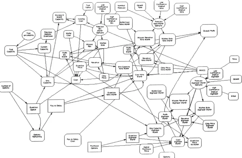
The full decision tree model is shown in Figure 11. This display is called an influence diagram. With an influence diagram the user can lay out each of the important variables in a model and set-up the flow between each of those variables. In addition, the major decisions of interest can be included in the model as well as any uncertainties that are tied to the model.
The flow of information is determined by the way in which the model is set-up. Constants are the first variables to have their information. The tree then works back from the final value, Overall Profit in this case, and determines which values need to be calculated first. The flow of the data and time is discussed in this section following the description of the overall model.
The full model shown below can be broken up into three separate sections. There is a section that deals with the immediate needs of the capacity. This is the six-month demand forecast that represents the actual expected demand six-months from today.
There is then a section that has a nine-month demand forecast and an eighteen-month demand forecast. These are the actual nine-month and eighteen-month expected demands.
CCAcrc
E wovd xcess 6 selgh
Capackvselen COP11ernce
-Si afef Cos t d
In* WcplWi od
Wo d Ok-Qrall "Cll
Tod Prvos Waler Demara
upcerwlpef Execrci Ca
CapEcacisea
Ninein Wod Aedwac
Owirerpt Prof
rodCpa i Eip*
CaWaclo Coost Cooiedp
111p EW ghese E T
EPrices CIIcie gamer
(1p
Wodo Cn* Prc"CPI" k--* d EE Ehw c
Oncec
Figure 12 shows the actual time flow for the purchase of a photolithography machine. The tool takes approximately 18-months, from the beginning of the manufacturing process to the delivery of the tool, to be completed. There are primarily two stages in the production of a photolithography machine. The first is the growing and polishing of the crystal that is used in the tool. This is the majority of the lead-time and is where most of the time is used. The second portion of the lead-time is the completion of the tool. This involves the assembly of the remaining components. There is a natural break 12-months into the process. The crystal is not specific to any one buyer and can be used in any tool. The remainder of the tool, however, may be specific to a certain buyer. So given these time constraints, any option would have to be exercised at a time of six-months.
Time = 3 Months Time =12 Months Time =18 Months
Beginning of the Beginning of the Tool Delivery
Manufacturing Final Manufacturing
Process Process
4 1 - Timrne
Figure 12. Critical Times
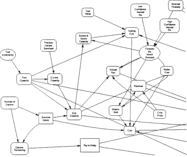
The portion of the tree that is in the six-month time frame is shown in Figure 13. This portion of the tree models the decisions and activities based on the forecast for demand six-months from now. Each of the variables in the tree is discussed in Section 4.2. In fact, each of the time frames looks similar with the differences being the time frame that each of the decisions are made in. In the six-month time frame, there are two decisions that are made. The first is the decision to exercise any options that are currently due. The second is, if these options are not exercised, should they be allowed to expire or
should they be delayed for a period. If the option is delayed, it is then active for the next six-month period.
This model would need to be run every three months. In other words, at time zero the user will enter the six-month forecast, the number of options that were exercised in the past, and the number of options that come due in this time period.
Confide
uVlw sitDenn
Capaky rfila
Cst
Figure 13. The Decision Tree for the Six-Month Time Frame
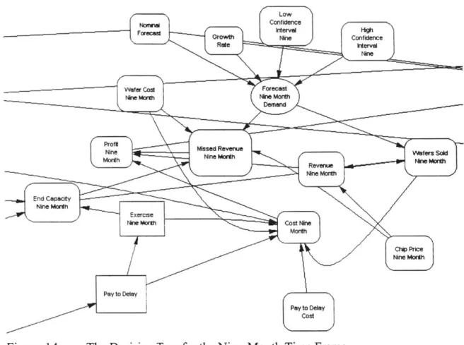
In addition, the user must enter the data for the nine-month time frame, which represents the decisions and activities based on the nine-month demand forecast. This is shown in Figure 14. The only data that needs to be entered at this time are the forecast for the nine-month time frame along with the various costs and prices.
Low
Noff" Confide
FT Growth Nine Confidence
Rete Interval
Wafer Cost Forecast
oe mret t ne Month
Demand
Prot ~ Missed Reveu
tie erod Nica pinsi sadng fore a toaWoa2motsteo er tbeomes Month Revenc Nine Month En Capacity We MorthCost Nine Monyth Nine Morth Pay to Delay-Pay to Delay cost
Figure 14. The Decision Tree for the Nine-Month Time Frame
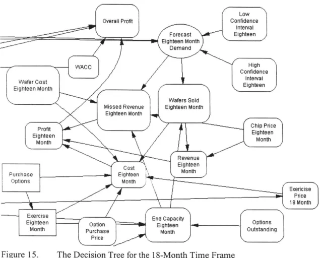
The user then enters the data for the 18-month time frame, which is shown in Figure 15. Again, this models the decisions and activities made in the current time period in response to the 18-month demand forecast. The user needs to enter a long-term forecast and the number of options on tools that are currently outstanding. For example, if an option is bought in the current time period then that option will be outstanding in the next time period. In fact, an options is outstanding for a total of 12-months before it becomes
Low
Overall Profit Confidence
Forecast Eghteen Eighteen Month
-- WACCConfidencey
Wafer Cost Interval
Eighteen Month Eighteen
Wafers Sold Missed Revenue Eighteen Month
Eighteen Month
P rofit Chip Price
Eighteen Eighteen
Month Month
Revenue
Cost Eighteen
Purchase i n avEighteen Month
Options Month Exericise Price 18 Month Exercise End CapacityOpin
Eighteen Option Eighteen -1Opttain
Month Purchase Month ttndg
Price
Figure 15. The Decision Tree for the 18-Month Time Frame
When the user has entered data for each of the time frames, the model can be run. Three-months later, the updated data will then be inputted and the model is run again.
4.1.1 Real-Time Flow
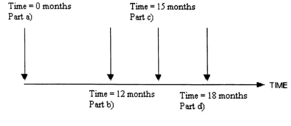
It is also important to have an understanding of what is happening in real-time before the model is described in detail. Figure 16 shows an 18-month delivery time for the
Time = 0 months Time = 15 months
Part a) Part c)
P TIME
Time = 12 months Time = 18 months
Part b) Palt d)
Figure 16. Real-Time
a) At time = 0 months, a decision is made to purchase options that can be exercised in 12 months. This decision is made based on the demand forecast for 18-months in the future and the amount of capacity that is currently available.
b) At time = 12 months, the 18-month forecast that was generated in step a) can now be updated to provide a new six-month forecast. This six-month forecast should be more accurate given that new information should have appeared over the past year. With this new six-month forecast, decisions are made as to how many of the options purchased in part a) should be exercised, how many should be delayed, and how many should expire.
c) At time = 15 months, the options that were delayed in part b) must either be exercised, delayed again, or left to expire. If the options are exercised then they will be delivered at time = 21 months.
d) At time = 18 months, the tools are delivered if there were options exercised in part b). The uncertainty in the tool production rate is realized as is the actual demand.
While these steps lay out what is happening in real time, it is important to realize that this is an ongoing process. In other words, at time = 0 above, a decision is made to purchase a certain number of options given the 18-month forecast. Three months later,
there is a new step a). This means that a new 18-month forecast is needed (21 months from the first forecast) to determine the number of options that are necessary, given the options already purchased, to make sure that there is enough capacity to meet demand. This is shown in Figure 17.
b
c d
a
T=O 1al
T=3
b
Cld-rii
n
a
43T=3*n
n n f ln 'IF TIMEFigure 17. Ongoing Real-Time
Figure 17 shows how the model flows in real-time when the model is run over and over again. At time = 0 months the data is put in the model and run. The decision is made
as to the number of options that should be purchased. At time = 3 months, the model is