Analyzing Upstream Impact on Downstream Shelf-Availability

Analyzing Upstream Impact on Downstream Shelf-Availability

by Xu Li

Bachelors, Business Administration, Nanjing Normal University, 2005

SUBMITTED TO THE PROGRAM IN SUPPLY CHAIN MANAGEMENT IN PARTIAL FULFILLMENT OF THE REQUIREMENTS FOR THE DEGREE OF

MASTER OF APPLIED SCIENCE IN SUPPLY CHAIN MANAGEMENT AT THE

MASSACHUSETTS INSTITUTE OF TECHNOLOGY JUNE 2018

© 2018 Xu Li. All rights reserved.

The author hereby grants to MIT permission to reproduce and to distribute publicly paper and electronic copies of this thesis document in whole or in part in any medium now known or hereafter created. Signature of Author...

Master of Applied Science in Supply Chain Management Program May 11, 2018 Certified by...

James Blayney Rice, Jr. Deputy Director, Center for Transportation & Logistics Capstone Project Advisor Certified by...

Sergio Alex Caballero Research Scientist, Center for Transportation & Logistics Capstone Project Co-Advisor Accepted by...

Dr. Yossi Sheffi Director, Center for Transportation and Logistics Elisha Gray II Professor of Engineering Systems Professor, Civil and Environmental Engineering

Analyzing Upstream Impact on Downstream Shelf-Availability

by

Xu Li

Submitted to the Engineering Systems Division on May 11, 2018 in Partial Fulfillment of the Requirements for

the Degree of Master of Applied Science in Supply Chain Management

Abstract

On-shelf availability (OSA) is key in the Consumer Packaged Goods (CPG) industry. In this project, out of stock (OOS) patterns are identified, grouped, and analyzed in order to gain meaningful insights to improve OSA. The approach is to normalize a time-series dataset, search for similar OOS patterns, and analyze some particular patterns. By focusing on a particular type of pattern, in which an OOS event happens within a pre-defined time period, some behaviors are observed from this study: first, as the time period is decreased (from 7 days to 4 days), the similar OOS pattern happens more frequently; second, a steep inventory drop appears to be an infrequent event, based on the sample dataset. The purpose of this study is to draw a common approach that could possibly be used by practitioners; the firm could possibly use the index and similarity search approach to identify patterns in all GTINs. The potential insights of this study are: first, stock outs don’t seem to be predictable based solely on DC data, since steep inventory drops appear to be infrequent events; and second, a firm could possibly use the identified patterns to connect point of sale data with OOS events and then identify the drivers of out of stocks.

Capstone Project Supervisor: James Blayney Rice, Jr.

Acknowledgements

Thank you to my wife, Irene, my son, Patrick, my mom, Jianhua Li, and the rest of my family for your unconditional support and abundant love. Thank you to the professors, staff, and my SCM classmates of 2018 at MIT for your fellowship and ideas.

I want to thank Jim Rice and Sergio Alex Caballero for coaching me in the last nine months and teaching me Python and many subjects. I also want to thank team members from my sponsor company for sharing your knowledge of both CPG industry and analytical projects, and Chris Caplice, Connor Makowski, and Francisco J. Jauffred from CTL for your lectures and inspiration.

Table of Contents

3.3 Normalized data using index ... 11

3.3.1 Matrix Profile ... 11

3.3.2 Modified method ... 13

3.3.3 Index and similarity search ... 14

3.3.4 Visualize data and eight patterns ... 15

4. Data Analysis and Results ... 16

4.1 Similarity search results for eight patterns ... 17

4.2 Three Patterns and behaviors ... 18

4.2.1 Pattern I gradually OOS ... 19

4.2.2 Pattern II Last for 3 days ... 22

4.2.3 Pattern III Last for 3 days then 2 days of OOS ... 24

4.3 Frequency of pattern I ... 24

4.4 Histogram and steep drop ... 26

5. Discussion ... 28

5.1 Initial approach-to compare with average inventory ... 28

5.2 Inventory in last two days ... 28

5.3 Links to store data... 29

5.4 Future studies ... 29

6. Conclusion ... 30

7. References... 31

8. Appendix ... 32

Table of Figures

Figure 2 Distance Profile (Mueen & Keogh 2016) ... 12

Figure 3 Matrix Profile (Mueen & Keogh 2016) ... 13

Figure 4 Matrix Profile index (Mueen & Keogh 2016) ... 13

Figure 5 Time series dataset for GTIN #1, with all 42 DCs ... 15

Figure 6 Frequency for eight different types of potential patterns ... 17

Figure 7 Pattern I gradually OOS in 7 Days ... 18

Figure 8 Samples of Pattern I (gradually OOS in 7 Days) ... 19

Figure 9 Original Time Series (Pattern I gradually OOS in 7 Days) ... 21

Figure 10 Pattern I inventory values ... 22

Figure 11 Pattern II inventory lasting for 3 days ... 22

Figure 12 Frequency of Pattern II (7, 6, 5 and 4 Days) ... 23

Figure 13 Pattern III inventory lasting for 3 days then 2 days of OOS ... 24

Figure 14 Pattern I inventory lasting for 3 days ... 26

Figure 15 Histogram of Pattern I ... 27

1. Introduction

Overview and objectives

The sponsor company is a global consumer packaged goods manufacturer (CPGM), headquartered in North America. The CPGM manufactures products, stores finished goods mainly in mixing centers, and ships to large retailers across the country. Shipments typically go to retailers’ distribution centers (DCs), and then products are distributed to each store from there.

The particular problem presented is that the CPGM’s retail customers have been facing frequent out of stock (OOS) events at their DCs. Typically, each product has a GTIN (Global Trade Item Number, a universally accepted unique identifier for each product being sold), and each GTIN is associated with 42 DCs. Stock outs could be more frequent at some DCs during certain time periods, such as holidays. The CPMG is concerned with OOS events because they can lead to lost sales.

The sponsor company believes that there is a pattern for inventory drops. The objective of this research is to identify whether there actually is an identifiable pattern, either sudden or gradual, especially in the last two days prior to the OOS event. If there is a sudden inventory drop in the two days prior to an OOS, then actions could possibly be taken to replenish inventory to the DCs in order to minimize the impact of an OOS.

For this project, one product line was studied. With inventory-level data provided by the CPGM, eight types of potential stock-out patterns were predefined and tested. Further study was based on three types of high-frequency patterns, including one in particular: inventory gradually decreasing to an OOS event within a certain number of days (7, 6, 5, and 4 days).

In order to identify a list of potential patterns, the study uses both index and similarity search methods. To avoid certain values dominating the whole dataset, the data is first normalized by converting each individual inventory value to an

index. The next step is to use a predefined range of indices to search for similar patterns in the new dataset. For a specific pattern, both an index and an absolute inventory value are used to identify when inventory is gradually declining without any replenishment shipment being received during the same time period.

What is an OOS?

There are two types of an out-of-stock event (OOS), each described in the following text.

Concept 1: An out-of-stock event (OOS) at the store level occurs when, for some time period, an item is not available for

sale on the shelf. If a retailer needs an item to be available for sale, but there is no physical presence of a salable unit on the shelf, then the item is deemed to be OOS. The OOS event begins when the final saleable unit of a GTIN is removed from the shelf, and it ends when a saleable unit on the shelf is replenished (Gruen & Corston 2008).

Concept 2: An OOS event at the DC level occurs when the inventory level is zero at a specific DC for a specific GTIN. In

the CPGM’s case, an OOS event at the DC level could lead to an OOS event at the store level. For instance, if a retailer’s DC runs out of inventory for a particular GTIN, then the associated stores that are replenished by that DC could possibly have an OOS event if the DC fails to replenish before the store experiences an OOS event. The store would then receive the inventory and put those items on the shelf. In this study, OOS events at the DC level were studied.

In the data analysis section, some observations and behaviors of three high-frequency patterns are described. Furthermore, in the discussion section, steep drops in inventory at the DC level were discussed and summarized using histograms, and some further research recommendations are presented.

2. Literature Review

This section gives an overview of prior published research that has consideted this problem. The Matrix Profile analysis method described by Yeh et al. (2016) of the Computer Science and Engineering department of the University of California Riverside is a time-series data-mining algorithm for pattern recognition. The reason to study a Matrix Profile is that it normalizes a dataset and converts each data point to an index (or Euclidean distance). Because the range of inventory values for the product studied greatly varies for different DCs and GTINs, it would be very difficult to search similar patterns using absolute inventory numbers. Furthermore, shapes, not exact value, are concerned in aggregating various patterns. In this research, a similar method was used to normalize datasets and then use the resulting indices to search similar patterns in new datasets. I propose to mimic the processes from the UCR Matrix Profile and modify the calculation for rapid analysis.

Pattern recognition and data mining are directly relevant to this research. Pattern recognition can take advantage of machine learning techniques that allow us to detect patterns, trends, and irregular events in data. With the growth in the number of data-mining and machine-learning techniques, patterns in data can be accurately recognized. These patterns could be used to create insights about customer behaviors and market trends. These insights are meant to allow a company to evaluate its internal management and operational practices and how they could be improved.

There are a number of methods and software programs that can be used for pattern recognition. Examples of such methods include Matrix Profile and Deep Neural Network (DNN); examples of software include Python, R, Minitab, SAS, and Tableau. This research focused on the Matrix Profile method. As previously mentioned, a Matrix Profile is a time-series data-mining algorithm. To begin with, a time time-series {Yt} or {y1,y2,⋯,yT} is a discrete, continuous-state process where time t=1,2,⋯,=T are certain discrete time points spaced at uniform time intervals (Imdadullah 2013). A Matrix Profile annotates a time series, solving problems such as motif discovery, density estimation, anomaly detection, rule discovery, joins, segmentation, clustering, etc. If there is a pattern that repeats frequently in the time-series dataset, it

would be useful to have a mechanism to recognize and capture it. A Matrix Profile attempts to identify what is repeated in a time series, when it appears and why an expected conservation was not observed (Yeh et al., 2016).

3. Methodology

In this section, datasets provided by the CPGM are described and further aggregated. Due to the complexity of the data structure and data volume, 20 representative GTINs were selected and further analyzed. In addition, the steps involved in the Matrix Profile are explained in greater detail. The modified approach for the index and similarity searches is introduced and used to identify and aggregate patterns in the sample dataset. Eight types of potential pattern are predefined and tested in the sample data, and three high-frequency patterns are focused on in this study. The three patterns are described and their behaviors are observed, setting the stage to focus on one particular pattern, which is gradually OOS within a certain number of days (7, 6, 5, and 4 days).

3.1

Data understanding

The data provided was divided into three types of files: DC data, ODS (order sales) data, and store data. Each file represents a different aspect of the same GTIN and DC combinations and contains one year’s worth of data, from July 2016 to June 2017.

1. DC data includes inventory on hand and out of stocks, representing daily inventory levels at any given date in a

specific DC for a specific GTIN. The daily inventory levels of 432 GTINs were recorded with the sales date, DC number, GTIN number, inventory on hand, OOS indicator, Push or Pull and brand of product.

2. ODS data includes transactions between the CPGM’s DC and the retailer’s DC. The data contains the date of order, DC

quantity, brand, description of the product’s dimensions and demand signal (base demand, promotion, initiative-phase in and phase out etc.).

3. Store data contains POS data at the store level, including the number of stores served by a certain DC for the GTIN being

studied, the DC number, average sales, average store inventory, average store daily sales, and number of stores out of stock.

3.2

Sample data

The entire dataset included 432 GTINs in 42 DCs labeled with five distinct demand signals:

1. Base Demand, the most stable demand, representing 80% of shipping volume and including a predictable base level of demand.

2. Unexpected Demand, which involves little advance notice from customers.

3. Phase In (New Product Introduction), when products are launched with no order history. The CPGM usually plans the introduction six months in advance.

4. Promotion, a planned peak in demand, when GTINs have a rapid increase in sales volume. 5. Phase Out, when an existing product becomes obsolete.

There are five brands in the whole dataset. One of them was selected for the sample data since it has the highest volume. This brand contains 144 GTINs, and 20 were selected for study based on two criteria, high volume and diversity of demand signals:

• High volume: The combined volume of 20 GTINs represents more than 50% of the total volume. • Diversity of demand signals: There are combinations of demand signals under each GTIN.

3.3

Normalizing data using an index

This section further introduces the Matrix Profile and a similar approach that is used to normalize datasets and perform similarity searches in sample datasets.

3.3.1

Matrix Profile

A Matrix Profile is a time-series data-mining algorithm. This method is used to normalize data and find similar behaviors within a dataset, which could be one or two time series. There are four steps in a producing a Matrix Profile, as described by Yeh et al. (2016):

1. The Euclidean distance uses z-normalized distance calculated between two time series;

2. The distance profile contains the z-normalized Euclidean distance between query and each subsequence by sliding a window of length m across the time series;

3. The Matrix Profile stores distance between each subsequence and its nearest neighbor; and

4. The Matrix Profile index is used to retrieve the location and distance of the nearest neighbor to any subsequence.

The Matrix Profile was chosen as the basis for developing a similar approach that normalizes data by converting it to an index and then performs a similarity search in each subset of the sample data. In this study, the m value is chosen to be 7, 6, 5, and 4 days. For the purpose of identifying and aggregating patterns, the first two steps of the Matrix Profile are modified for use in this study.

As described by Yeh et al. (2016), the following is an example of using a Matrix Profile for a time series T. A time series T includes a sequence of value: T = t1, t2, ..., tn where n is the length of T. A subsequence Ti,m of T is a continuous subset of T, with length m starting from position i. Thus: Ti,m = ti, ti+1,…, ti+m-1, where 1 ≤ i ≤ n-m+1. The distance can be computed between any selected subsequence to all sequences, by normalizing the value of T and calculating the Euclidean distance between two time series (see Figure 1).

Figure 1 Z-normalized Euclidean Distance (Mueen & Keogh 2016)

A distance profile (see Figure 2) records Euclidean distances between a Ti,m and each subsequence in T, which is set {T1,m,, T2,m,…, Tn-m+1,m} by sliding a window of length m across T, where m is a predefined length. For each subsequence Ti,m, there will be a nearest neighbor relationship between two subsequences (Yeh et al., 2016).

Figure 2 Distance Profile (Mueen & Keogh 2016)

With the nearest neighbor relation between two subsequences, a Matrix Profile (see Figure 3) records Euclidean distances between each combination of the nearest neighbor of subsequences for the two time series TA and TB. At the same time, a Matrix Profile index (see Figure 4) records the locations of all subsequences’ nearest neighbors for TA and TB. Essentially

the Matrix Profile and the Matrix Profile index annotate a time series TA with the distance and location of all its subsequences’ nearest neighbors in itself or another time series TB (Yeh et al., 2016).

Figure 3 Matrix Profile (Mueen & Keogh 2016)

Figure 4 Matrix Profile index (Mueen & Keogh 2016)

3.3.2

Modified method

This research did not apply the same methodology used for aggregating patterns and conducting a similarity search. Since SQL and Python were preferred in this research, the index and similarity searches were developed in a Python environment. Furthermore, Matlab is not capable of quickly implementing and scaling in the sponsor company’s working

environment. Normalizing the data method and a brute force method for the similarity search were distilled from the Matrix Profile.

The following are some key definitions:

• Index is calculated by comparing the inventory level of a specific day to the average inventory level of the interval (m days). Index=Inventory level Ti / (Average Inventory (Ti to Ti+m-1)).

• Moving average is an all-subsequences set A of a time series T in an ordered set of all possible subsequences of T, obtained by sliding a window of length m across T: A ={T1,m,, T2,m,…, Tn-m+1,m}, starting with Ti then moving to Ti+1, Ti+2,,,T358.

• Lower bound and upper bound are set as a range of an index.

• Similarity search uses a range of an index developed from identified patterns; the index is then matched in a new dataset to the existing index’s interval, which indicates a similar pattern I in the same dataset.

• The m value is chosen to be 7, 6, 5, and 4 (days).

3.3.3

Index and similarity searches

In order to describe and sustain shapes of different patterns, the concept of the index is further developed. By

normalizing the inventory value in the DC data, each absolute inventory number is transformed to an index with a range between 0 and 7. Since I have predefined the lower bound and upper bound of each row, searching an index in a new dataset could be conducted within the index’s range.

To begin with, the dataset for each GTIN contains information for all 42 DCs, with each DC containing one year’s worth of time-series data points. As a result, one GTIN-DC combination includes 365 days of data points, and there are 42 DCs for each GTIN, totaling 15,330 rows under one GTIN. Then there are five steps in order to search similar patterns:

1. Calculate the average inventory level within each subset of time series (length of subset=m); 2. Divide each inventory level by the average inventory level in order to obtain the index for each row;

3. Compare each index to the interval of the predefined index range: If each index is within the lower bound and upper bound of the predefined index range, then a pattern is identified, indicated, and recorded in the new dataset;

4. Slide the subset until the end of the time series in the same DC data; and 5. Repeat the same steps for all 42 DCs’ data.

Essentially, I repeat the same steps for all 20 representative GTINs. Furthermore, Python is used for this specific calculation (see Appendix 1). It takes about 20 minutes to calculate one GTIN and export files with indicators of similar patterns.

3.3.4

Visualize data and eight patterns

Figure 5 is a good way to demonstrate the need to conduct a similarity search using an index. Figure 5 visualizes time-series data for a specific GTIN # 1, containing all 42 DCs. It would be nearly impossible to manually go through each DC for each GTIN over one year’s worth of data to detect a series of potential patterns, not to mention that there are 432 unique GTINs in the given product family. The range of inventory value is between 0 and 600, which makes pattern recognition even harder.

Figure 5 Time series dataset for GTIN #1, with all 42 DCs

Eight different types of patterns (see Appendix 2) were preselected based on the initial observations and feedback from the sponsor company. For instance, Patterns 1, 3, 4, 5, and 7 describe how long inventory can last until the next stock out and whether replenishments could be associated with a single or a series of stock outs, whereas Patterns 2, 6 and 8 focus on behaviors between stock outs and replenishment orders. (Pattern 1, 4 and 7 will be discussed further in this research.) In order to maintain the shape of a specific pattern, in each pattern type, seven days of inventory data is collected from the sample data then normalized using the index method. Further, the lower bound and upper bound are both defined so that the similarity search can be performed in the new dataset.

4. Data Analysis and Results

In this section, the results of eight patterns are presented and compared after the similarity search is conducted. Furthermore, three out of eight patterns are analyzed and studied, and some key observations are presented. For Pattern I (gradual OOS), the frequency under different m values (7, 6, 5, and 4 days) is compared for several GTINs. The

main reason to focus on Pattern I is that when the m value changes, both Pattern II and Pattern III will change shapes. However, Pattern I still maintains the same shape and only becomes shorter in length.

4.1

Similarity search results for eight patterns

After defining all eight different patterns (see Appendix 2), the similarity search is conducted using ranges of index value. This search method is tested with five unique GTINs for all 42 DCs. Initial observations indicate that certain patterns happen more frequently than others. For example, Patterns 1, 4, and 7 are relatively high-frequency patterns among all eight patterns. Also, as the m value decreases from 7 days to 4 days, similar pattern shapes happen more often (see Figure 6).

Figure 6 Frequency for eight different types of potential patterns

4.2

Three patterns and behaviors

Based on the preliminary findings and testing, three representative patterns were selected and further analyzed. Pattern I represents behavior where inventory decreases before OOS, without any replenishment order during the same time period. Patterns II and III show the potential impacts of the number of OOS days when the inventory lasts for three days and then is out of stock.

4.2.1

Pattern I Gradually Out of Stock

Pattern I: The inventory level gradually decreases towards zero (within 7, 6, 5, and 4 days). There is no replenishment

order within the defined time interval (see Figure 7). A gradually decreasing Pattern I is captured by two criteria: index and absolute value. In this example, the index dropped from 2.24 to 0 from Day 1 to Day 7. For the calculation, the lower and upper bounds are set from 0.01 to 7 from Day 1 to Day 6 and 0 for Day 7. Besides the index, the inventory-on-hand value is also compared to ensure the previous value is always higher than the next day’s inventory value. Based on both criteria, a gradually declining Pattern I can be captured.

Figure 7 Pattern I gradually OOS in 7 Days

Behavior of Pattern I: For Pattern I, the most important question is without a replenishment shipment, how fast the

inventory level can decrease to zero. Different time intervals are tested, with 7, 6, 5, and 4 days, respectively. One observation is that the shorter the time interval, the more frequent Pattern I is captured in the same GTIN file. Second, for the 7-days scenario, inventory drops appear to be skewed left, based on the sample dataset. However, as the m value becomes smaller, from 7 to 4, inventory drops appear to be moving towards the center and becoming more symmetric.

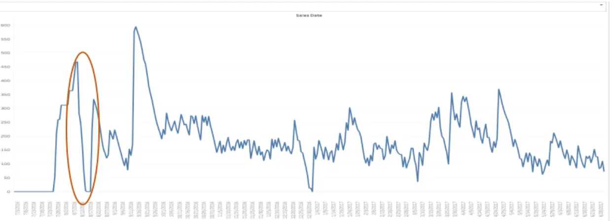
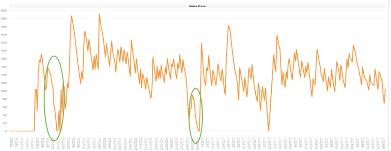
Figure 8 Samples of Pattern I in index (gradually OOS in 7 Days)

The above two graphs (see Figure 8) show aggregated Pattern I and associated index value for various GTINs. As shown in Figure 8, three sample patterns are circled, whereas the original time series (see Figure 9) are also presented in order to give a perspective of how the original dataset behaves. As shown in Figure 9, Pattern I highlighted in red appears in GTIN # 1 DC #1; the same pattern is circled in red in Figure 8. Another two types of Pattern I appear in the same GTIN #1 and DC #2 (see Figure 9); the same patterns are circled in green in Figure 8.

Figure 9 Original Time Series (Pattern I in GTIN # 1 DC #2)

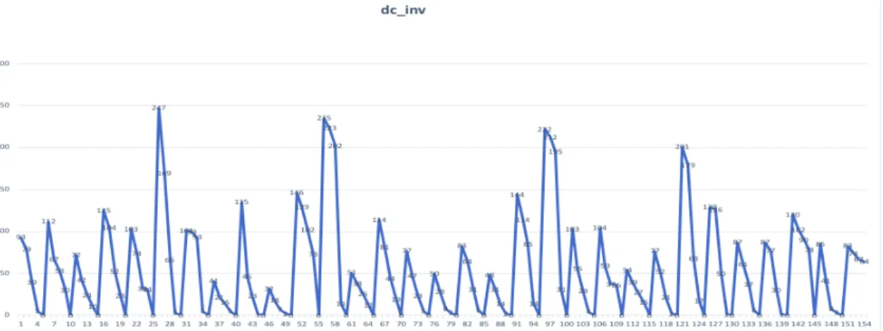
Furthermore, as the m value decreases (from 6 days to 4 days), Pattern I appears more frequently, as shown below in Figure 10.

Figure 10 Pattern I inventory value (gradually OOS in 5 Days)

Figure 10 Pattern I inventory value (gradually OOS in 4 Days)

4.2.2

Pattern II Lasting for 3 days

Pattern II: In this pattern, the inventory lasts for three days, and on the fourth day the inventory is out of stock (see

Figure 11). The replenishment occurs on the fifth day, and the inventory lasts for at least another three days. In this scenario, there is a one-day OOS event but the replenishment order was able to “catch” the stock out and minimize the impact at the store inventory level.

Figure 11 Pattern II inventory lasting for 3 days

Behavior of Pattern II: Inventory levels are not always parallel three days prior to the OOS and three days after the OOS.

There might be multiple replenishment shipments after the OOS, which needs to be further investigated and analyzed.

Furthermore, this pattern appears to occur as frequently as Pattern I (see Figure 12). Especially when the time interval is reduced to 3 days, with at least one day above moving average and one day below moving average, this pattern

happens even more frequently than Pattern I.

4.2.3

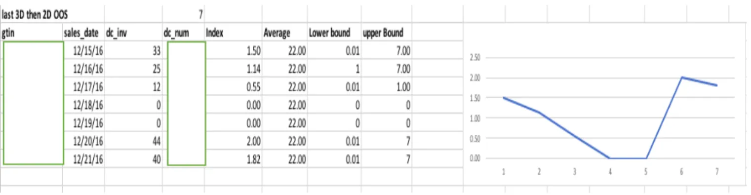
Pattern III Inventory lasting for 3 days, then 2 days of out of stock

Pattern III: The inventory level gradually reduces to zero within 3 days and is followed by two days of stock out (see

Figure 13).

Figure 13 Pattern III inventory lasting for 3 days then 2 days of OOS

Behavior of Pattern III: compared to Pattern II, the replenishment appears to fluctuate with greater magnitude. One of

the reasons might be that following two days of stock outs, a heavy replenishment is typically ordered, in order to avoid another OOS event.

4.3

Frequency of Pattern I

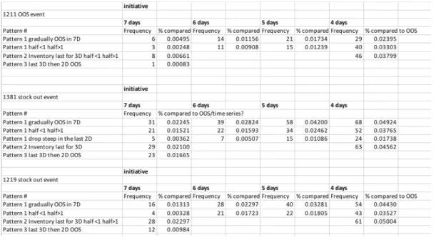
By changing the time interval from 7 days to 4 days, the frequency increases as the m value becomes smaller. However, it is necessary to point out that the same patterns do repeat among various GTINs. In this example, there are 6 different instances of Pattern I in GTIN # 3, when the m value equals 7. By reducing the m value to 6 days, there are 14 different instances of Pattern I, which include portions of 6 occurrences of Pattern I from the 7-days scenario. The same situation happens in the 5-days and 4-days scenarios. As shown below, the frequency for Pattern I is presented for various GTINs.

The frequency is calculated as the number of identified patterns compared to the total number of OOS events (see Figure 14).

Figure 14 Pattern I inventory lasting for 3 days

4.4

Histogram and steep drops

As mentioned earlier in the introduction section, the hypothesis of this research is that if there is a pattern for a sudden inventory drop, then the OOS could potentially be monitored and predicted and actions could be taken to minimize the impacts of OOS. In this study, the inventory drop of the last two days is compared to the inventory level’s starting point. For instance, for a particular Pattern I starting with 142 units of inventory, at Day 5 only 53 units are left in that DC, meaning that 37% of the total inventory dropped on Day 5 and Day 6 prior to the OOS event. With the calculated percentage, a histogram is further developed (see Figure 15). For GTIN # 3, the inventory drop that is between 0 and 20% occurs twice; the inventory drop between 20% and 40% occurs four times.

A steep drop is also defined as: for the 7- and 6-days patterns, the inventory reduces by more than 70% for the last two days prior to OOS; for the 5-days pattern, the inventory reduces by more than 80% for the last two days prior to OOS. Based on all 20 GTINs (see Appendix 3), steep drops are infrequent events, since the frequency is less than 10%.

5. Discussion

The core question for Pattern I is how fast the inventory drops before OOS events. If the inventory drops faster in the last few days prior to OOS, the OOS event could potentially be predicted and the firm could possibly take preventive action.

Two approaches are explored to define what is considered to be a steep drop. First, each inventory value is compared with the average inventory level. This is widely used by major retailers, and the benefit is a quick check and simple rule of thumb. Second, the inventory drops for the last two days were compared for all 20 sample GTINs. If the inventory decreases much faster in the last two days, then the OOS event might be predicted. Based on the results of two approaches, steep drops appear to be infrequent events.

5.1

Initial approach-to compare with the average inventory

In order to find out how fast the inventory drops, the first step was to further break down patterns to two stages before a stock out: In the 7-days scenario, the first stage is the first 3 days with the inventory level higher than the average of the 7 days, and the second stage is the following 3 days with the inventory level lower than the average. This particular scenario implies that once the inventory level is lower than the average, within 3 days OOS events might occur. By studying this scenario, the OOS signal could be further linked to lead time and safety stock. One implication could be that the CPMG has 3 days to react before the OOS event. In order to capture the gradually downward trend, the indices need to be defined as: between 1 and 7 for the first three days, between 0.01 and 1 for the following three days, and 0 for the last day.

5.2

Inventory in the last two days

After discussions with the sponsor company, it was decided to focus on the last two days prior to the OOS, instead of three days. A steep drop is defined as: for the 7 and 6-days scenarios, the inventory drops by more than 70% in the last two days, whereas for the 5-days scenario, 80% is the threshold for a steep drop. Based on this assumption, all 20 GTINs

are analyzed and summarized using histograms (see Appendix 3). Based on the results, steep drops seem to be infrequent events (less than 10%).

5.3

Links to store data

During this study, store-level data was also analyzed and compared to Pattern I. One of the interesting findings is that POS data could be either higher or lower than the inventory starting level for the 7-days pattern (see Figure 16).

Figure 16 Pattern I joined DC and Store dataset

This pattern happened several times within the 63 days of the dataset, as shown in Figure 12. Meanwhile, the total store inventory level is still higher than the POS number, which implies that the inventory was not sufficiently distributed to the right stores. Accordingly, safety stock could be further communicated and discussed between the CPGM and retailers.

5.4

Future studies

On top of this, demand signals could also be factored in by adding more GTINs and comparing the difference in behaviors among the five types of demand signals.

Another potential path would be to add the frequency of inventory dropping to zero within one day. Since 7, 6, 5, and 4 days of Pattern I are studied, 2 days (the first day with inventory and the next day OOS) could be valuable. This could easily be done by changing the index to the first day between 0.01 and 7 and the following day to 0.

5.5

Limitations

One of the limitations of this research approach is that both the index and the absolute inventory value are used in the similarity search. For instance, in order to maintain the trend of inventory gradually decreasing until OOS, the inventory on-hand value is compared to ensure that the later inventory position is always lower than the previous one. Future studies could only use indices for the same purpose.

6. Conclusion

Using the index and similarity search methods, a series of OOS patterns can be identified and aggregated in a large scale. Instead of manually going through each time series, a pattern can be generalized and described using both the index and the absolute inventory value. By studying a specific pattern, gradually OOS, it was found that steep drops seem to be infrequent events. The findings further indicate that stock outs don’t seem to be predictable based solely on the DC data. Using the identified Pattern I dataset, store data could be further explored to draw links between the POS and OOS. Essentially, the firm could possibly use the index and similarity search methods to test more potential patterns and GTINs, and then aggregate by the GTIN-DC combinations. This method could possibly be scaled to all 432 GTINs to aggregate patterns from 4 million transactions, with an output of small sets of repeated patterns. Based on the smaller dataset, the firm may be able to identify the drivers of out of stocks by connecting the POS data with OOS events.

7. References

Gruen, T. W., and Corsten, D. (2008). A Comprehensive Guide To Retail Out-of-Stock Reduction in the Fast-Moving

Consumer Goods Industry (University of Colorado at Colorado Springs)

Imdadullah, M. (2013). Time Series Analysis and Forecasting: http://itfeature.com/time-series-analysis-and-forecasting/time-series-analysis-forecasting

Mueen, A., and Keogh, E. (2016). Matrix_Profile_Tutorial_Part1&2:http://www.cs.ucr.edu/~eamonn/MatrixProfile.html Yeh, C. M., Zhu, Y., Ulanova, L., Begum, N., Ding, Y., Dau, H., Silva, D. F., Mueen, A., and Keogh, E. (2016). Matrix Profile I:

All Pairs Similarity Joins for Time Series: A Unifying View that Includes Motifs, Discords and Shapelets (University

8. Appendix

Appendix B Eight Patterns

Pattern 1 the inventory gradually decreasing till OOS in 7 days. This pattern is about how fast the inventory drops with one replenishment.

Pattern 2 the inventory lasts for two days; the OOS occurs on the third day; a heavy replenishment occurs on the fourth day and the OOS lasts for three consecutive days. This pattern could imply that even a relative “heavy” replenishment couldn’t fulfill the demand and that the replenishment was not generated timely.

Pattern 3 the inventory lasts for two days, the OOS occurs and then a replenishment lasts for only two days. Is the inventory only lasting for two days a frequent or infrequent event?

Pattern 4 the inventory lasts for three days, the OOS occurs, and then a replenishment lasts for three days. Is inventory lasting for three days a frequent or infrequent event?

Pattern 5 the inventory lasts for three days and then the OOS lasts for two days; a replenishment occurs and only lasts for one day, and then the OOS occurs on the last day. Is there a strong demand signal that causes two OOS events and one replenishment couldn’t provide the sufficient inventory?

Pattern 6 a repetitive pattern with the replenishment lasting one day and the OOS the following day. Does OOS event tend to cluster?

Pattern 7 the inventory lasts for three days; the OOS occurs for two days; a replenishment occurs and lasts for two days. This is a comparison with the pattern 4 to evaluate the relationship between the magnitude of OOS and the

replenishment behavior following the OOS event.

Pattern 8 the inventory doesn’t move for three days; the OOS occurs and lasts for two days; a replenishment occurs and lasts for two days. Is there a heavy demand signal that consumes all inventory within one day?