Data-driven Pricing and Inventory Management
with Applications in Fashion Retail
by
Mila Nambiar
Submitted to the Sloan School of Management
in partial fulfillment of the requirements for the degree of
Doctor of Philosophy in Operations Research
at the
MASSACHUSETTS INSTITUTE OF TECHNOLOGY
September 2019
@Massachusetts
Institute of Technology 2019. All rights reserved.
Signature redacted
A u th or ...
...
Sloan School of Management
August 9, 2019
Signature redacted
C ertified by ...
...
David Simchi-Levi
Professor
Thesis Supervisor
Accepted by
...
Signature
redacted
MASSACHUSETTS INSTITUTE
Patrick Jaillet
OFTECHNOLOGY
Professor
SEP 0 5 201g
Co-director, Operations Research Center
Data-driven Pricing and Inventory Management with
Applications in Fashion Retail
by
Mila Nambiar
Submitted to the Sloan School of Management on July 10, 2019, in partial fulfillment of the
requirements for the degree of
Doctor of Philosophy in Operations Research
Abstract
Fashion retail is typically characterized by (1) high demand uncertainty and products with short life cycles, which complicates demand forecasting, and (2) low salvage values and long supply lead times, which penalizes for inaccurate demand forecasting. In this thesis, we are interested in the design of algorithms that leverage fashion retail data to improve demand forecasting, and that make revenue-maximizing or cost-minimizing pricing and inventory management decisions.
First, we study a multi-period dynamic pricing problem with feature information. We are especially interested in demand model misspecification, and show that it can lead to price endogeneity, and hence inconsistent price elasticity estimates and sub-optimal pricing decisions. We propose a "random price shock" (RPS) algorithm that combines instrumental variables, well known in econometrics, with online learning, in order to simultaneously estimate demand and optimize revenue. We demonstrate strong theoretical guarantees on the regret of RPS for both IID and non ID features, and numerically validate the algorithm's performance on synthetic data.
Next, we present a case study in collaboration with Oracle Retail. We extend RPS to incorporate common business constraints such as markdown pricing and in-ventory constraints. We then conduct a counterfactual analysis where we simulate the algorithm's performance using fashion retail data. Our analysis estimates that the RPS algorithm will increase by 2-7% relative to current practice.
Finally, we study an inventory allocation problem in a single-warehouse multiple-retailer setting with lost sales. We show that under general conditions this problem is convex, and that a Lagrangian relaxation-based approach can be applied to solve it in a computationally tractable, and near-optimal way. This analysis allows us to prove structural results that give insights into how the allocation policy should depend on factors such as the retailer demand distributions, and demand learning.
Thesis Supervisor: David Simchi-Levi Title: Professor
Acknowledgments
First and foremost, I would like to thank my advisor, David Simchi-Levi. David has always inspired me with his energy, and with his vision for how research ideas can grow and take shape as compelling stories. At the same time, he has constantly challenged me to become a clearer and more effective thinker and communicator. This thesis, and my growth as a researcher, would not have been possible without his support.
I would also like to thank the other members of my thesis committee, John
Tsit-siklis and Steven Graves, for taking the time to ask detailed questions, and to share suggestions and feedback that have shaped this thesis.
Next, a big thank you must go to the co-authors of the works in this thesis. Chapters 2-4 are joint work with my advisor, David Simchi-Levi, and He Wang. I would like to thank He Wang for working with me throughout these years, and for graciously hosting me at Georgia Tech earlier this year to work on the material in Chapter 4. I have learned a lot from his knowledge and experience, and from his creativity in and intuition for problem solving. I would also like to thank Su-Ming Wu and Setareh Borjian from Oracle Retail Global Business Unit, who are co-authors on the work in Chapter 3. I am grateful to them for taking the time to share their experience with revenue management practice with me. Their suggestions and feedback have been invaluable in designing the numerical experiments in this chapter.
Finally, I would like to thank some friends who have been especially supportive during this process: Ying Qiao Hee, Nathan Watson and Delphine Watson, for coming all the way from LA just to attend my defense, Rushabh Shah, Peter Yun Zhang, Charmaine Chia, and Xuewei Loy, for always checking in on me, and of course, my best friend and partner Ben Simon, for his unconditional support.
Contents
1 Introduction 15
2 Dynamic Learning and Pricing with Model Misspecification 19
2.1 Introduction . . . . 20
2.1.1 O verview . . . . 22
2.1.2 Background and Literature Review . . . . 24
2.2 M odel . . . . 28
2.2.1 Applications of the Model . . . . 30
2.2.2 Model Misspecification and Non-anticipating Pricing Policies . 31 2.2.3 Price Endogeneity Caused by Model Misspecification and Other Factors . . . . 32
2.3 Random Price Shock Algorithm . . . . 34
2.3.1 Performance Metric and Regret Bound . . . . 37
2.3.2 A Upper Bound of Regret . . . . 39
2.3.3 A Lower Bound on Regret . . . . 40
2.3.4 Price Ladder . . . . 41
2.3.5 Non-IID features . . . . 43
2.4 Numerical Results . . . . 47
2.5 C onclusion . . . . 55
3 Feature-based Dynamic Pricing for Fashion Retail: A Case Study 57 3.1 Introduction . . . . 57
3.2 3.3
Objectives and Assumptions . . . . Solution Approach: The Random Price Shock Algorithm
3.3.1 Legacy Pricing Process . . . .
3.3.2 The Random Price Shock Algorithm . . . .
3.4 Experimental Design . . . . 3.4.1 Data Processing . . . . 3.4.2 Demand Model . . . . 3.4.3 Estimation and Endogeneity. .. 3.4.4 Alternative Demand Models.... 3.4.5 Selecting Markdown Period Lengths
3.5 Simulation Results . . . . 3.6 Conclusion . . . . . . . . . . . . . . . . . . . . . . . . and other Parameters . . . . . . . . 4 Inventory Allocation with Demand Learning for Seasonal Goods
4.1 Introduction 4.1.1 Litera 4.1.2 Notati 4.2 Model . . . 4.2.1 Dema 4.3 Heuristic . . 4.3.1 Algori 4.3.2 An 01 4.4 Structural Re 4.4.1 Dema 4.4.2 Nonid 4.5 Numerical Ex 4.5.1 Dema 4.5.2 Non-id 4.6 Conclusion . ture Review . . . . on . . . . . . . .
ad Models with Learning/Forecasting . . . . .t i . . . .. thm . . . . timality Bound . . . . su lts . . . . nd learning . . . . entical retailers . . . . periments . . . . ad learning . . . . entical retailers . . . . . . . . 5 Conclusions and Future Directions
8 62 64 64 66 68 70 71 72 75 76 79 80 85 . . . . 86 . . . . 89 . . . . 93 . . . . 93 . . . . 95 . . . . 96 . . . . 97 . . . . 100 . . . . 101 . . . . 102 . . . . 104 106 . . . . 106 108 . . . . 110 113
A Appendix to Chapter 2 (Dynamic Learning and Pricing with Model
Misspecification) 115
A.1 A Different Regret Definition ... 115
A.2 Additional Numerical Results ... 116
A.2.1 Dependence of regret on the demand function . . . . 117
A.2.2 A.2.3 A.3 Proofs A.3.1 A.3.2 A.3.3 A.3.4 A.3.5 A.3.6 A.3.7 Dependence of regret on the feature vector Regret relative to different clairvoyants . . for Theoretical Analysis . . . . Proof of Proposition 1 . . . . Proof of Theorem 1 . . . . Proof of Theorem 2 . . . . Proof of Theorem 3. . . . . Proof of Proposition 2 . . . . Proof of Theorem 4. . . . . Lem m as . . . . dimension m . . . 118 . . . . 120 . . . . 122 . . . . 122 . . . . 123 . . . . 128 131 133 134 139 B Appendix to Chapter 3 (Feature-based Dynamic Pricing for Fashion Retail: A Case Study) 149 C Appendix to Chapter 4 (Inventory Allocation with Demand Learn-ing for Seasonal Consumer Goods) 155 C.1 Proofs for theoretical analysis . . . . 155
C.1.1 Proof of Lemma 1 . . . . 155
C.1.2 Proof of Theorem 5 . . . . 158
C.1.3 Proof of Theorem 6 . . . . 159
List of Figures
2-1 The dynamics of parameter estimates under model misspecification. . 21
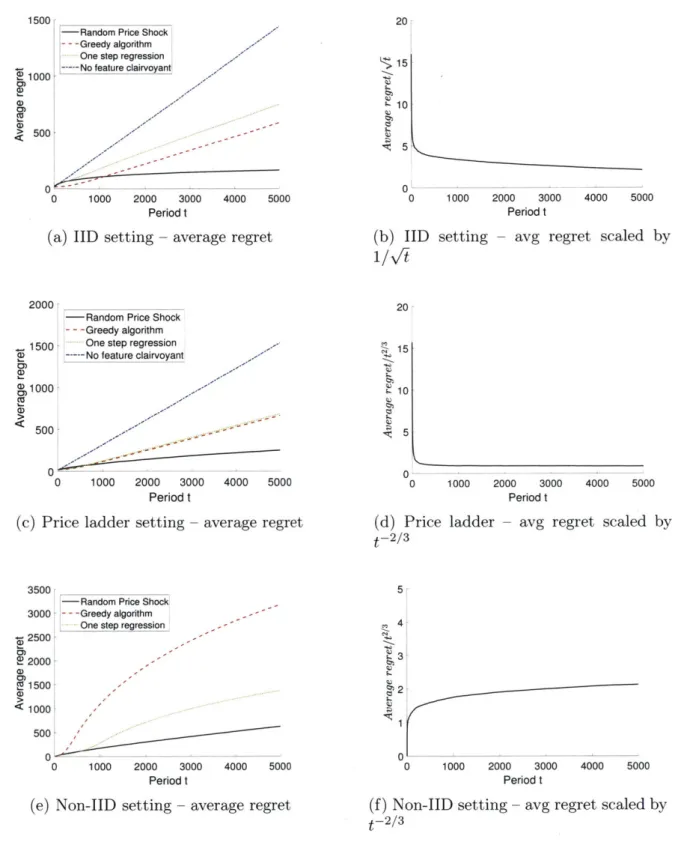
2-2 Average regret and scaled regret in IID, price ladder and non IID settings 54
3-1 Seasonality of demand . . . . 71
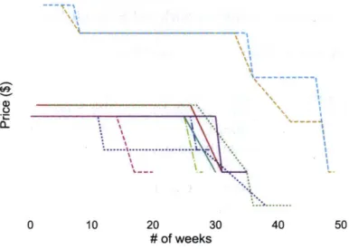
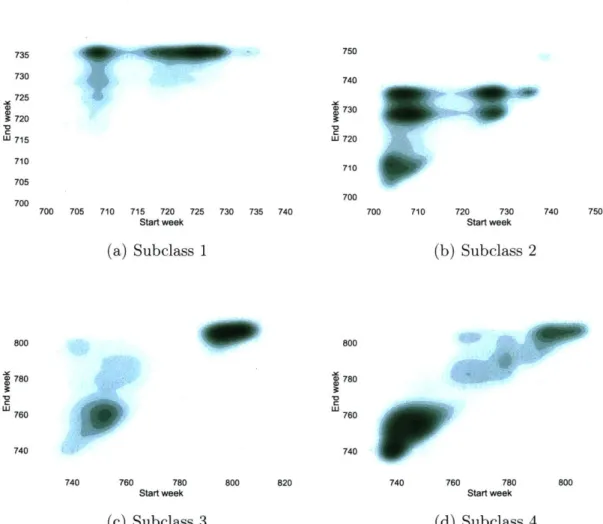
3-2 Markdown pricing: each trajectory represents the price of one item from the category . . . . 73 3-3 Kernel density estimation plots showing the distributions of the sales
start and end weeks for different products across all four subclasses . 78
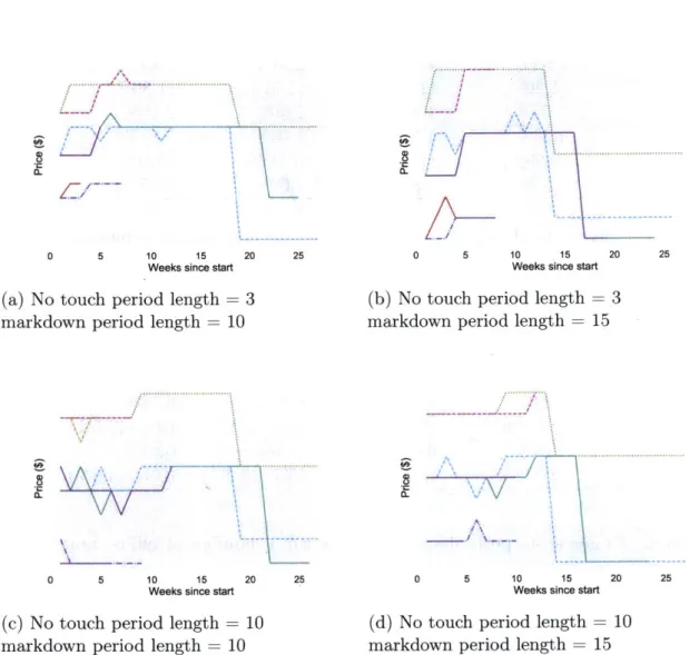
3-4 Price trajectories of the RPS heuristic for a sample of 10 products from Subclass 2 . . . . 81
4-1 First period optimal and approximate allocations for fixed starting warehouse inventory, wo,1 = 12, prices = $1, holding costs = $0.20, and
p = 0, 0.2, 0.4, 0.6, 0.8, 1. In both the truncated normal and uniform
demand settings, period 2 demand noise Ei,1 is drawn from a truncated
normal distribution with parameters y = 0, a = 1, a = -1, b= 1 . . . 109
4-2 First period allocations under the heuristic in a setting with 3 retail-ers, all off whom experience demand drawn from truncated normal distributions with parameters p,cou,a,b (retailer i's demands Di,t are
normally distributed according to
N(p,
2u), conditional on Di,tbe-longing to the range [a b].) For Retailer 1, the 'low variance retailer',
y = 2, = 0.1, a = 1, b = 3. For Retailer 2, the 'mid variance
re-tailer', p= 2, a -= 1, a = 1, b = 3, and for Retailer 3, the 'high variance
A-1 f(x) vs best linear approximation a
+
c'x for y = 1.02, 2 . . . . 117 A-2 Average regret over 50 iterations of RPS vs one-stage regressionalgo-rithm s as y is varied . . . . 119
A-3 Average regret over 10 iterations of the RPS algorithm as m is increased
from 1 to 1001. . . . . 120
A-4 Average regret over 200 iterations of RPS algorithm relative to two different clairvoyants in IID and Price ladder LID settings . . . . 121 B-i Average revenue over 100 iterations of different algorithms . . . . 153
List of Tables
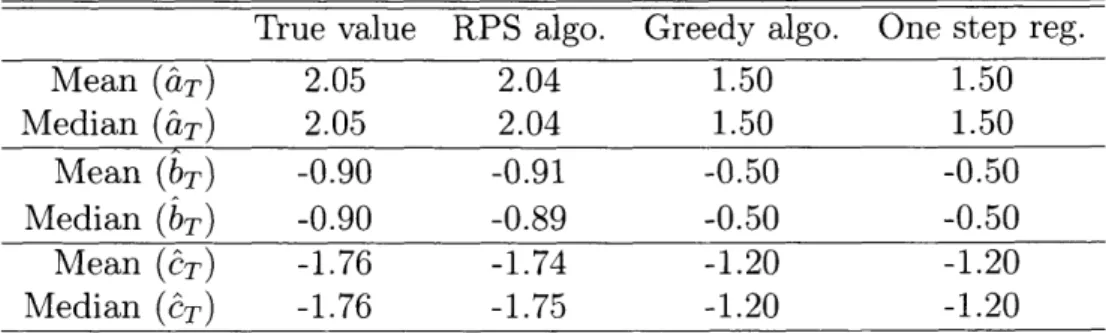
2.1 End of selling horizon parameter estimates in the IID setting ... 53 2.2 End of selling horizon parameter estimates in the price ladder setting 53
2.3 End of selling horizon parameter estimates in the non IID setting . . 53
3.1 Price coefficient estimates (95% confidence interval estimates in paren-theses) . . . . 74
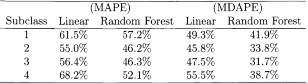
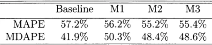
3.2 Demand prediction errors using different demand models . . . . 75 3.3 Test set errors of alternate models on Subclass 1 . . . . 76
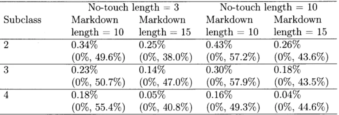
3.4 Revenue gains relative to current practice (Mean, 95% confidence in-terval estimates in parentheses) . . . . 82 3.5 Inventory clearance (Mean, 95 percentile and max in parentheses) . . 82
A.1 Estimates of parameter b in Linear Demand Example . . . . 118
B.1 Estimates of parameter b (with 95% confidence interval) . . . . 154 B.2 Comparison of estimated revenues earned by various algorithms (with
Chapter 1
Introduction
In this thesis, we are interested in pricing and inventory management problems that arise in fashion retail. Among retail applications, fashion retail is unique for a number of reasons. Most distinctive is the seasonality of fashion retail: Every season, new product lines are introduced at stores, sold for only around 10 weeks, then removed from stores (Fisher and Raman, 1996).
Also, the amount of inventory available during each season tends to be fixed. This is because items have to be shipped across long distances, from the countries where they are manufactured, to reach stores located in the US, Europe, etc. Since
supply lead times are long relative to the product lifecycles, replenishments during
the short selling seasons are thus either not possible, or are limited in number. For
example, at the Spain-based fast fashion retailer Zara, which is one of the largest
fashion retailers today, initial shipments from the production to distribution centers before the start of each season make up around half of the total volume of available
inventory during each season (Gallien et al., 2017).
A third defining characteristic of fashion retail is that items that are not sold to
customers by the end of each season are resold at very low salvage values. These salvage values tend to be much lower than the full prices of the items, and may even
be lower than the cost of production (Fisher and Raman, 1996).
Given these factors, fashion retailers face two big challenges: For one, it is difficult
amount of information is available on the sales of each product. At the same time, since inventory is fixed and salvage values are low, inaccurate demand forecasting, or inadequate planning to meet demand, can lead to costly lost sales opportunities.
The three parts of this thesis address these various challenges in fashion retail by proposing data-driven algorithms that make use of the kinds of data that are available
to fashion retailers - such as transaction and item feature data - to perform more
accurate demand forecasting, and to consequently make better pricing and inventory management decisions. We are particularly interested in algorithms that "learn and earn" on the fly, meaning that learning and optimization take place simultaneously rather than in separate stages. As additional sales or demand data is observed, it is used to update the retailer's demand forecasts, and to then make pricing or inventory management decisions that generate demand, and so on and so forth. Since product lifecycles are so short in fashion retail, incorporating the most recent data in demand forecasting is essential to making more accurate predictions.
Another strategy that fashion retailers can use to improve their demand forecast-ing for products with short lifecycles is feature-based pricforecast-ing. Rather than considerforecast-ing each item in isolation, fashion retailers can look at the sales of products with similar characteristics, i.e. products that are in the same category, and that share similar features such as color, brand, design pattern ete, and that are therefore likely to ex-perience similar demands. These kinds of item feature data can be combined with transaction data in order to perform demand estimation and make pricing decisions. Large fashion retailers, such as Zara and its closest competitors H&M and Forever 21, where the number of new articles of clothing released every year are in the thousands
(Caro and Gallien, 2012), especially stand to benefit from feature-based pricing. Chapters 2 and 3 of this thesis study feature-based pricing, the former from a theoretical perspective, and the latter from the point of view of the company Oracle Retail, which is a business unit of Oracle and a leading provider of software and IT solutions to retailers. In Chapter 2, Dynamic learning and pricing with model mis-specification, we show that one of the pitfalls of designing a dynamic pricing policy when demand depends on feature information lies in correctly estimating the causal
relationship between demand and price. For example, if the policy assumes a mis-specified demand model, either because the decision maker is unsure of how demand is affected by the features, or of how to model such a dependence, demand noise can become correlated with the price (price endogeneity). Price endogeneity then leads to biased estimates of the demand-price relationship, and results in suboptimal pricing decisions. Another factor that can lead to price endogeneity is that pricing managers at companies may choose admissible price sets based on their own beliefs of future demand, and in response to demand factors such as product quality, trendiness, etc., that are unobservable to the algorithm.
In Chapter 2, we thus propose a "random price shock" (RPS) algorithm that manages these pitfalls by dynamically generating randomized price shocks to estimate price elasticity while maximizing revenue. We show that the RPS algorithm has strong theoretical performance guarantees, that it is robust to model misspecification, and that it can be adapted to a number of business settings, including (1) when the feasible price set is a price ladder, and (2) when the contextual information is not IID. We also perform numerical experiments on synthetic data to gauge the performance of RPS, and find that it significantly outperforms competing algorithms that do not account for price endogeneity.
In Chapter 3, Feature-based dynamic pricing with for fashion retail: A case study, we adapt the RPS algorithm to be broadly applicable to fashion retail settings. We keep the price experimentation structure of the RPS algorithm proposed in Chapter 2, but modify it to incorporate business constraints faced by many fashion retailers, such as fixed inventory and markdown pricing constraints. The modified algorithm makes use of intuitive and computationally tractable approximations to optimize the retailer's total expected revenue subject to these constraints. To gauge its perfor-mance, we have run a number of offline numerical experiments using retail data from one of Oracle Retail's clients. The heuristic exhibits revenue gains of around 2-7% over current practice, and seems robust to different retailer parameter settings such as the length of the markdown and no-touch periods.
alloca-tion. We study an inventory allocation problem in a two-echelon (single-warehouse multiple-retailer) setting with lost sales. At the start of a finite selling season, a fixed amount of inventory is available at the warehouse, and can be allocated to the retailers over the course of the selling horizon with the objective of minimizing total expected lost sales costs and holding costs. We allow each retailer to experience cor-related demands, and show how this framework can capture learning in the sense of demand forecasting (e.g. ARMA) model, as well as a Bayesian learning mdoel.
Then, we pose the questions of (1) how to solve the inventory allocation problem under demand learning in a computationally tractable way, and (2) how demand learn-ing impacts effective inventory allocation policies. To address the first question, we adapt the Lagrangian relaxation-based technique proposed by Marklund and Rosling (2012) for a backordering, no-learning setting. We show under general assumptions that the resulting heuristic remains near-optimal in our setting, compared to the orig-inal dynamic program. Forig-inally, we use this analysis to investigate the relationship between demand learning and early allocation decisions. Through a combination of theoretical and numerical analysis, we show our main result: Demand learning has a similar effect as risk pooling on inventory allocation policies, as it provides an in-centive for the decision maker to withhold inventory at the warehouse rather than allocating it in earlier periods.
Chapter 2
Dynamic Learning and Pricing with
Model Misspecification
We study a multi-period dynamic pricing problem with contextual information where the seller uses a misspecified demand model. The seller sequentially observes past demand, updates model parameters, and then chooses the price for the next period based on time-varying features. We show that model misspecification leads to corre-lation between price and prediction error of demand per period, which in turn leads to inconsistent price elasticity estimate and hence suboptimal pricing decisions. We propose a "random price shock" (RPS) algorithm that dynamically generates ran-domized price shocks to estimate price elasticity while maximizing revenue. We show that the RPS algorithm has strong theoretical performance guarantees, that it is ro-bust to model misspecification, and that it can be adapted to a number of business settings, including (1) when the feasible price set is a price ladder, and (2) when the contextual information is not ID. We also perform numerical experiments gauging the performance of RPS on synthetic data, and find that it significantly outperforms competing algorithms that do not account for price endogeneity.
2.1
Introduction
Motivated by the growing availability of data in many revenue management applica-tions, we consider a dynamic pricing problem for a data-rich environment. In such an environment, a firm (i.e., seller) observes some time-varying contextual information or features that encode external information. The firm estimates demand as a func-tion of both price and features, and chooses price to maximize revenue. By including features into demand models, the firm can potentially obtain more accurate demand forecasts and achieve higher revenues.
In this work, we are especially interested in the consequences of model
misspec-ification, namely, when the firm assumes an incorrect demand function on features.
In practice, features may contain various kinds of information about demand such as product characteristics, customer types, and economic conditions of the market. A mixed set of heterogeneous features can affect demand in a complex way. The seller may assume an incorrect demand model either because it is unsure how demand is affected by features, or because it prefers a simple model for analytical tractability. In fact, several recent works on dynamic pricing with features make the assumption that demand is a linear or generalized linear function of features (Cohen et al., 2016; Qiang and Bayati, 2016; Javanmard and Nazerzadeh, 2016; Ban and Keskin, 2017).
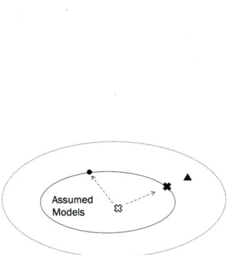
We observe that when the demand model is misspecified, model parameters es-timated from demand data may become biased and inconsistent. This phenomenon is illustrated in Fig. 2-1 below. In this figure, the inner oval represents a parametric family of demand models assumed by the seller. The white "x" mark represents the seller's initial parameter estimation. The triangle mark represents the true model, which lies outside the oval region, since the model assumed by the seller is misspeci-fied. Over time, as the seller collects past demand data and updates demand model parameters, one would expect that the updated parameters would converge to the best approximation of the true model (denoted by a solid "x" dot on the boundary, i.e., the projection of the triangle mark to the oval region). Under some assumptions, the model with the best approximation is also the one associated with the highest
Assumed Models
Figure 2-1: The dynamics of parameter estimates under model misspecification.
revenue performance within the assumed model family (see Sometimes, the updated model parameter (circle dot) may even have worse revenue performance than the initial model estimation (white "x")!
The reason why the estimated parameters are inconsistent is that model misspec-ification can cause correlation between the price and demand prediction error. We refer to this correlation effect as price endogeneity. If an estimation method ignores the endogeneity effect and naively treats the assumed model as the true model, it would produce biased estimates. Note that we use the word "endogeneity" here in a pure statistical sense, indicating that an independent variable is correlated with the error term in a linear regression model (Greene, 2003).
In this work, we will mainly focus on the price endogeneity effect caused by model misspecification; however, a discussion of all possible factors that may cause price endogeneity is beyond our scope.
2.1.1
Overview
To illustrate the price endogeneity effect caused by model misspecification, we specifi-cally consider a dynamic pricing setting where the true demand model is quasi-linear, in that the expected demand is linear in price but nonlinear with respect to features. The seller does not know the underlying demand function, and incorrectly assumes that the demand function is linear in both price and features.
To address the issue of model misspecification, we propose a "random price shock" (RPS) algorithm that is able to obtain unbiased and consistent estimates of the model parameters while controlling for the price endogeneity effect. The idea of the RPS algorithm is to add random price perturbations to "greedy prices" recommended by some price optimization model using biased parameter estimates. The variances of these price perturbations are carefully controlled by the algorithm to balance the so-called exploration-exploitation tradeoff. Intuitively, using a larger variance can help explore and learn the demand function, while using a smaller variance can generate a price that is closer to greedy prices, which can exploit current parameter estimates to maximize revenue.
The RPS algorithm is related to three types of methods in econometrics and op-erations management for demand estimation. First, the RPS algorithm is in some sense similar to the randomized controlled trials (RCT) method, which offers ran-domly generated prices to eliminate selection bias. For example, Fisher et al. (2017) applies RCT in a field experiment to estimate an online retailer's demand model. However, it is important to note a key difference between RPS algorithm and the RCT method: the price offered by RPS algorithm is not completely random, because it is the sum of a greedy price, which is endogenous, and a small perturbation. As a result, the sum of the two prices is also endogenous; therefore, standard analysis for randomized control trials cannot be applied to the RPS algorithm. Moreover, Fisher et al. (2017) implemented RCT in two phases: a first phase where random prices are offered, and a second phase where optimized prices are tested. In contrast, the RPS algorithm does not have these two phases, and it estimates the demand model
while optimizing price. The benefit of estimating demand and optimizing price con-currently is discussed in Besbes and Zeevi (2009); Wang et al. (2014). The analysis of the RPS algorithm is also significantly different from that of RCT, and the proof idea for the RPS algorithm is built on the analysis of the least squares method in nonlinear models (Hsu et al., 2014).
The second type of method that is related to the RPS algorithm is the instrumental variables (IV) method. Instrumental variables is a widely used econometric method to obtain unbiased estimates of coefficients of endogenous variables. It aims at finding the so-called instrumental variables that are correlated with endogenous variables but are uncorrelated with prediction error. In the RPS algorithm, the randomly generated price perturbation serves as an instrumental variable, because it is correlated with an endogenous variable, i.e., the actual price offered by the firm (recall that the actual price is the sum of a greedy price and a perturbation), but is obviously uncorrelated with prediction error since it is randomly generated by a computer. This connection to instrumental variables allows us to use econometrics tools in the design of RPS algorithm, more specifically the two-stage least squares (2SLS) method.
Lastly, the RPS algorithm is related to the family of "semi-myopic" pricing policies that has been studied in the revenue management literature more recently (Keskin and Zeevi, 2014; den Boer and Zwart, 2013; Besbes and Zeevi, 2015). A semi-myopic pricing policy keeps track of whether there has been sufficient variations in historical prices; if not, an adjustment is made such that the actual price offered would deviate from greedy or myopic price. Our proposed RPS algorithm belongs to the family of myopic policies. However, it is important to note that most existing semi-myopic algorithms make deterministic price adjustments to the greedy prices, whereas the RPS algorithm makes randomized price adjustments. This is a major difference since our ability to perform unbiased parameter estimation in the presence of price endogeneity heavily relies on the fact that those price perturbations are randomized. In Section 2.3, we show that the RPS algorithm accurately identifies the "best" linear approximation to the true quasi-linear model in the presence of model misspec-ification. The algorithm achieves an expected regret of O((1+ m)v T) compared to
a clairvoyant who knows the best linear approximation, where m is the dimension of features and T is the number of periods. Our regret bound matches the best possi-ble lower bound of
Q(V)
that any non-anticipating algorithm can possibly achieve. Moreover, RPS improves theO(Vlog
T) regret bound proven by Keskin and Zeevi(2014) for a special case of linear models without features (i.e., m = 0).
Two extensions of the RPS algorithm are considered. In the first extension, we consider the case where prices must be chosen from a discrete set. We establish a
O(T2/3) regret bound for this generalized setting. In the second extension, we remove
the assumption that feature vectors are drawn IID, and allow them to be sampled from an arbitrary distribution. Again, a O(T2/3) regret bound is shown.
Finally, we test the numerical performance of the RPS algorithm using synthetic data in Section 2.4. These experiments demonstrate that the RPS algorithm obtains unbiased estimation in the presence of price endogeneity, and shows that it outper-forms other pricing algorithms proposed in the literature, which do not account for price endogeneity.
2.1.2
Background and Literature Review
Demand model misspecification is a common problem faced by managers in revenue management practice (Kuhlmann, 2004). Cooper et al. (2006) have discussed several reasons why model misspecification can arise, including revenue managers' lack of understanding of the pricing problem, or their preference for simplified models for the sake of analytical tractability.
Several previous papers study the consequences of model misspecification in dy-namic pricing. Cooper et al. (2006) study a problem where an airline revenue manager updates seat protection levels sequentially using historical booking data. The revenue manager incorrectly assumes that customer demand is exogenous and independent, but because the true demands for different fare-classes are substitutable, the booking data is affected by the manager's own control policy. Cooper et al. show that when an incorrect demand model is assumed, the firm's revenues would systematically de-crease over time to the worst possible values for a broad class of statistical learning
methods, resulting in a so-called "spiral down effect." On a high level, the spiral-down effect discovered by Cooper et al. (2006) is analogous to the phenomenon we illus-trated in Fig. 2-1: As more data is collected, ignoring model misspecification in the estimation process increases bias in parameter estimates over time, and the seller's revenues deteriorates. Besbes and Zeevi (2015) consider a single product dynamic pricing problem in which the seller uses a linear demand function to approximate the unknown, nonlinear true demand function. The authors have proposed a learning algorithm that would converge to the optimal price of the true model. Cooper et al.
(2015) consider an oligopoly pricing setting where firms face competition from each
other, but their demand models do not explicitly incorporate other firm's decisions. The authors have studied conditions under which the firms' decisions would converge to Nash equilibria. We note that in these three papers, demand function is assumed to be stationary. Instead, we consider a setting where demand function is affected by features, which are changing over time.
The effect of model misspecification on decision making has also been studied in other operations management applications. For example, Dana Jr. and Petruzzi (2001) study a newsvendor problem where the customer demand distribution depends on the inventory stock level chosen by an inventory manager, but the manager in-correctly assumes that demand distribution is exogenous. Cachon and K6k (2007) consider a newsvendor model where the salvage value is endogenously determined
by remaining inventory, while the inventory manager assumes the salvage value is
exogenous.
We consider a setting where the demand model contains unknown parameters that are being estimated dynamically from sales data. In such a setting, the firm faces an exploration-exploitation tradeoff: towards the beginning of the selling season, it may test different prices to learn the unknown parameters; over time, the firm can exploit the parameter estimations to set a price that maximizes revenue. Our problem setting is closely related to the one considered by Keskin and Zeevi (2014). They study a linear demand model without features, and consider a class of semi-myopic algorithms that introduce appropriately chosen deviations to the greedy price
in order to maximize revenue. Keskin and Zeevi show that this class of algorithms has the optimal regret rate, i.e., no other pricing policy can earn higher expected revenue asymptotically (up to a logarithmic factor). Another related paper is den Boer and Zwart (2013), which proposes a quasi-maximum-likelihood-based pricing policy that dynamically controls the empirical variances of the price. Besbes and Zeevi (2009) and Wang et al. (2014) consider dynamic pricing for a single problem under an unknown nonparametric demand model. Besbes and Zeevi (2012) extend the previous result to a setting with multiple products and multiple resources under an unknown nonparametric demand model. For an overview of some of the other problem settings and solution techniques used in dynamic learning and pricing, we refer readers to the recent survey by den Boer (2015).
We are particularly focused on a dynamic learning and pricing problem that con-tains contextual information (i.e. features). In related work on dynamic pricing with features, Qiang and Bayati (2016) extend the linear demand model in Keskin and Zeevi (2014) to incorporate features, and apply a greedy least squares method to estimate model parameters. Cohen et al. (2016) propose a feature-based pricing algorithm to estimate model parameters when demand is binary. Javanmard and Nazerzadeh (2016) and Ban and Keskin (2017) study pricing problems where feature vector is high dimensional and the demand parameter has some sparsity structure. We note that all these papers assume that demand models are correctly specified. In contrast, we study a feature-based pricing problem where the model is misspecified,
and focuses on the impact of model misspecification on the seller's revenue. Among these papers, Qiang and Bayati (2016) and Ban and Keskin (2017) are closest to our work as they both consider linear demand models with features. Nevertheless, due to the differences in model assumptions, the regret bounds in Qiang and Bayati (2016)
(O(logT)), Ban and Keskin (2017) (O(vTlogT)) and this paper (O(VY)) cannot
be directly compared. In particular, Qiang and Bayati (2016) make an "incumbent price" assumption, which gives the firm more information initially and allows the firm to achieve a much lower regret bound of O(log T) rather than O(T).
We note that a few recent papers apply nonparametric statistical learning
proaches to pricing with features in a batch learning setting where historical data are given as input (Chen et al., 2015; Bertsimas and Kallus, 2016). These works differ from ours in that we focus on a dynamic, multi-period setting. As stated in Van Ryzin and McGill (2000) and Cooper et al.
(2006),
in revenue management practice, there is usually a repeated process where controls (e.g., booking limits or prices) are en-acted, new data are observed, and parameter estimates are updated. In this work, we are specifically interested in the case where historical data is dynamically generated the seller's pricing decisions. In addition, although nonparametric approaches avoid model misspecification, parametric models are widely used in revenue management practice (Kuhlmann, 2004; Cooper et al., 2006; Besbes and Zeevi, 2015), so the con-sequence of model misspecification remains highly relevant to revenue management practice.As mentioned earlier, model misspecification can cause price endogeneity, because the demand prediction error and the seller's pricing decisions are both determined endogenously by the feature vector. More generally, the phenomenon of price endo-geneity are extensively studied in economics, marketing, and operations management. Empirical studies have found that price endogeneity exists and has a significant im-pact on price elasticity estimation in many real-world business settings (Bijmolt et al.,
2005). The econometrics literature has proposed various methods to identify model
parameters with endogeneity effect (e.g. Greene, 2003; Angrist and Pischke, 2008); Talluri and Van Ryzin (2005) also provides an overview of these methods with rev-enue management applications. The price endogeneity effect has been studied in settings with consumer choice (Berry et al., 1995), consumer strategic behavior (Li et al., 2014), and competition (Berry et al., 1995; Li et al., 2016); these factors are beyond the scope of this paper. We note that empirical revenue management studies often take the perspective of an econometrician who is outside the firm and does not observe all the information that revenue managers can observe, such as cost, product characteristics, consumer features, etc. (e.g. Phillips et al., 2015). However, we take the perspective of a revenue manager within the firm who makes pricing decisions, much like in Cooper et al. (2006) and Besbes and Zeevi (2015). We show that even if a
decision maker observes all the past pricing decisions, untruncated historical demand and contextual information, price endogeneity can still arise when the seller assumes an incorrect model.
Notation
For two sequences {an} and {bn} (n = 1,2,...), we write an= O(bn) if there exists
a constant C such that a, < Cbn for all n; we write an = Q(bs) is there exists a constant c such that an> cbn for all n. All vectors in this chapter are understood to be column vectors. For any vector x E Rk, we denote its transpose by xT and denote its Euclidean norm by ||x|| := VxTx. We let ||xj|1 be the f1 norm of x, defined as
xlli = E |xil. We let ||x||- be the £2 norm, defined as ||x||, = maxi
lxt|.
For anysquare matrix M E Rkxk, we denote its transpose by MT, its inverse by M-1 and its trace by tr(M); if M is also symmetric (M = MT), we denote its largest eigenvalue
by Amax(M) and its smallest eigenvalue by Amin(M). We let |IMI2 be the spectral norm of matrix M, defined by JMI2 = Am(MTM). We denote the Frobenius normofMbyllM||F,namely|MH|F= ftr(MTM).
2.2
Model
We consider a firm (seller) selling a single product over finite horizon. At the beginning of each time period (t = 1, 2, ... ,T), the seller observes a feature vector, xt E R',
which represents exogenous information that may affect demand in the current period. We assume that feature vectors xt are sampled independently for t = 1, 2,.. ., T from
a fixed but unknown distribution with bounded support. (In Section 2.3.5, we will relax the IID assumption on the features and assume an arbitrary sequence of random feature vectors.) Without loss of generality, we assume xt E [-1, 1]" after appropriate
scaling. Moreover, we assume that the matrix
M= E[[ i ]
is positive definite.1
Given the feature vector xt, customer demand for period t as a function of price
p is given by
Dt(p) = bp +
f
(xt) -+ et, Vp E [tp, t]. (2.1) Here, parameter b is a constant representing price sensitivity of customer demand,and
f
: R" -+ R is a function that measures the effect of features on customerdemand. Both b and
f
are unknown to the seller. We assume that the demand function is strictly decreasing in price p (i.e. b < 0), and f(xt) is bounded for allxt such that If(xt) <
f.
The latter assumption would follow immediately from thefact that the set of all features xt is compact if
f were continuous. The last term et
in Eq (2.1) represents a demand noise. Without loss of generality, we assume et has zero mean conditional of xt: E[t|
xt] = 0; otherwise, the conditional mean E[et I xt]can be shifted into function
f(xt).
We assume that et has bounded second moment (E[e] < o2 ,Vt), and is independent of historical data (x,, E,) for all 1 t s t - 1.However, the distribution of et is allowed to vary over time. We refer to Eq (2.1) as a
quasi-linear demand model, since the demand function is linear with respect to price,
but is possibly nonlinear with respect to features.
We denote the admissible price range in period t, i.e. the range of prices from which the price p must be chosen, by [p,, pt]. In particular, we allow the admissible price interval to vary over time. We assume that p, and pt are inputs to the seller's decision problem, while they may be arbitrarily correlated with features xt and demand noise
et. We also assume there exist constants 6 > 0 and pmx such that pt Pmax and
Pt - p, > 5 for all t. Given features xt, we denote the optimal price for the true
demand model (as a function of xt) by Pt(xt) (xt). 2b We assume that the optimal
price Pt(xt) c [p, pt] for all t.
This assumption is equivalent to the condition of "no perfect collinearity," i.e., no variable in the feature vector can be expressed as an affine function of the other variables. If matrix M is not positive definite, the dimension of feature vector can be reduced by replacing certain variable as a combination of other variables.
2.2.1
Applications of the Model
The above model has applications in several business settings that involve feature-based dynamic pricing. One example is dynamic pricing for fashion retail, which will be discussed in more detail in Chapter 3. In the fashion retail setting, a retail manager dynamically sets prices for fashion items throughout a selling season, while the demand is highly uncertain when the selling season begins. The feature vectors represent the characteristics of fashion items, such as color and design pattern, as well as seasonality variables. Throughout the season, the retail manager may learn from sales data about how customer demand varies for different product features, and adjust prices accordingly to maximize revenue. Another example of an application of feature-based pricing is personalized financial services. Phillips et al. (2015) describe a setting in the auto loan context, where the price (interest rate for a loan) is adjusted based on features such as credit score of the buyer, the amount and term of the loan, the type of vehicle purchased, etc. They find that using a centralized, data-driven pricing algorithm could improve profits significantly over the current practice, where local salespeople are granted discretion to negotiate price. In our model, the admissible price interval t, pt] is allowed to vary for different periods. For example, in the auto loan context, the price interval represents the range of admissible interest rates set by the financial headquarters, which varies based on the amount and term of the loan offered. As time-varying bounds may depend on features and demand noise, our model makes no assumption of the distribution of price range ,pt], and allows the price bounds to be arbitrarily correlated with past prices, feature vector xt, and noise Et. If such a correlation is present, it will lead to price endogeneity (in addition to the price endogeneity caused by model misspecification) and will be accounted for in our pricing algorithm.
30
2.2.2
Model Misspecification and Non-anticipating Pricing
Poli-cies
We consider a seller who is either unaware that the true demand function has a nonlinear dependence on features, or is unsure how to model such dependence. As a result, the seller uses a misspecified linear demand function to approximate the true quasi-linear demand function given by Eq (2.1). The seller assumes a linear demand model as
Dt(p) = a + bp + cTxt + VtI, Vp E ,Pt], (2.2)
where a E R and c E R" are constants and vt is an error term.
We focus on the linear demand model, because the linear model and its variations are widely used in revenue management practice and in the demand learning literature (Qiang and Bayati, 2016; Ban and Keskin, 2017); in addition, the model can capture nonlinear factors in the feature vector by including higher order terms in the feature vector.
The parameters (a, b, c) are unknown to the seller at the beginning of the selling season. We assume that the seller knows that the parameters a and c are bounded, and that there exist a, such that jal <
a
and 1|clb < c, but do not assume that the seller knows the values of aI . As for the price sensitivity parameter b, we assume that the seller knows not only that the parameter b is bounded, but also the range within which b lies, 0 < b < |b| b. The assumption that the range of b is known to the seller is strong, and is indeed a limitation of our model. However, there are applications for which it may be reasonable to assume that the seller has some knowledge about this range, perhaps from her prior experience with the sales of similar items during previous selling seasons. For example, in our case study in Chapter 3, where we apply our demand model to a fashion retail setting, our estimates of b for different categories of fashion items were found to be of the same order of magnitude, lying in the range[-1,
-0.1]. Thus the seller could assume that b lies in the range[-1,
-0.11for future selling seasons. More generally, the economics and marketing literature finds that price elasticity, a quantity related to our price sensitivity parameter, tends
to fall within finite ranges across markets and products. Bijmolt et al. (2005), for example, analyze 1851 price elasticities from 81 different publications between 1961 and 2004, across different products, markets and countries. They observe a mean price elasticity of -2.62 and find that the distribution is strongly peaked, with 50 percent of the observations between -1 and -3.
The seller must select a price pt E [p,,pt] for each period t = 1, 2,..., T sequen-tially while estimating the values of (a, b, c) using realized demand data. The seller's objective is to maximize her total expected revenue over T periods.
We denote the realized demand given pt by dt, defined as
dt = Dt(pt) = bpt +
f(xt)
+ ct.Note that the realized demand is generated from the true model, i.e., the quasi-linear model Eq (2.1).
The history up to the end of period t - 1 is defined as
Wt-1 = (x1, pi, Ei, . . . , xt_1, pt_1, Et_1).
We say that 7r is a non-anticipating pricing policy if for any t, price pt is a measurable function with respect to Wt-1 and the current feature vector and the feasible price
range: Pt= 7r(7it-1, xt, p, pt). The seller cannot foresee the future and is restricted
to using non-anticipating pricing policies.
2.2.3
Price Endogeneity Caused by Model Misspecification
and Other Factors
By comparing the true quasi-linear demand model (cf. Eq (2.1)) and the misspecified
linear model (cf. Eq (2.2)), it is easily verified that the error term in the misspecified
linear model is equal to vt =
f(xt)
- (a + cTxt) + et. This error term vi is composedof an approximation error,
f(xt)
- (a+
cTxt), which is correlated with features xt, and a random noise Et, which is uncorrelated with the features. When the modelis misspecified, we have
f(xt)
- (a + cTxt) / 0, so the error term vt is not meanindependent of feature xt, namely E[vt I xt]
#
0.The fact that the error term is not mean independent of the features could cause bias in the seller's demand estimates if the estimation procedure is not designed properly. Suppose the seller uses a non-anticipating pricing policy7r suchthat
Pt =_ r (t_1I, Xt, pt, Pt). (2.3)
Because the error term vt is correlated with the features xt while price pt is a function of xt, the seller's pricing decision causes a correlation between vt and pt. More
specifically, we have E[vtpt]
#
0 since E[vtpt I xt] = E[vt . 7r(Nti_,xt,P,pt) | xt] f 0. We refer to the correlation between pt and the error term vt as the price endogeneity effect, and refer to pt as the endogenous variable. Throughout this chapter, the word "endogeneity" is used in a pure econometric sense to indicate the correlation betweenpt and vt.
It is well known that in a linear regression model
dt = a
+
bpt + cTxt + vi, (2.4)when the regressor pt is endogenous, naive estimation methods such as ordinary least squares (OLS) would give biased and inconsistent estimates of parameters (a, b, c).
Biased estimates of model parameters then lead to suboptimal pricing decisions. Moreover, the seller cannot test whether price pt and error vt are correlated using historical data, since she does not observe the error term vt directly; even if the seller has complete historical data, without knowing the values of (a, b, c), the term
vt cannot be computed.
In addition to model misspecification, other factors can also cause the price en-dogeneity effect. If a manager believes she has expert knowledge about future de-mand, she may set the price range
[pt,,p]
in anticipation of future demand, so the price bounds p ,pt are endogenous. Because our pricing algorithm chooses price pt in[p,,pt],
the price pt also becomes endogenous. In our algorithm proposed inSec-tion 2.3, we account for such endogeneity by allowing the price bounds t, pt to be correlated with noise ct.
The endogeneity problem has been extensively studied in the econometrics lit-erature (Greene, 2003; Angrist and Pischke, 2008). There are a few key differences between the pricing model considered in this work and typical research problems studied in econometrics. First, we study a pricing problem from the perspective of a firm that wants to maximize its revenue, whereas econometricians often take the perspective of a researcher who is outside the firm and wants to estimate causal effects of model parameters. The second key difference is that econometrics and empirical studies often consider batch data, whereas our pricing model considers sequential data generated from dynamic pricing decisions. Analyzing these two types of data usu-ally requires different statistical methods and correspondingly different performance metrics.
Although there are differences between the problem considered in this work and those in the econometrics and empirical literature, a common challenge is in studying a regression model with endogenous independent variables. In fact, the dynamic pricing algorithm that we introduce in the next section is inspired by statistical tools in econometrics such as instrumental variables and two-stage least squares.
2.3
Random Price Shock Algorithm
In this section, we propose a dynamic pricing algorithm which we call the random
price shock (RPS) algorithm. The idea behind the RPS algorithm is that the seller can
add a random price shock to the greedy price obtained from the current parameter estimates. As the number of periods (T) grows, the parameters estimated by the RPS algorithm are guaranteed to converge to the "best" parameters within the linear demand model family, which we will define shortly in Section 2.3.1. Therefore, the prices chosen by the RPS algorithm will also converge to the optimal prices under the misspecified linear demand model.
We present the RPS algorithm below (Algorithm 1). The RPS algorithm starts 34
Algorithm 1 Random Price Shock (RPS) algorithm. input: parameter bound on b, B = [-,-b]
initialize: set &I = 0,b 1 = -b, 1 = 0
for t 1, ... , Tdo
set ot +-At-I2
given xt, set unconstrained greedy price: p,"t +- b+
project greedy price: pg,t - Proj(pu,, [pt + tpt - Jt])
generate an independent random variable Apt-
o
w.p.j
andAt < t w.p. 1
set price pt <- pg,t + Apt
choose an arbitrary price pt E [pI pt] observe demand dt = Dt(pt)
set bt+1 <- Proj(- ,pd B)
set (&t+1, t+1) <- arg min 2 1(ds - bt+ips- a- -YTxS) 2 end for
each period by choosing a perturbation factor
ot.
The algorithm computes the greedy price, pg,, and adds it to a random price shock, Apt. Note that the greedy price isprojected to the interval [pt +
ot,pt
- 6t], so that the sum of greedy price and priceshock is always in the feasible price range [p,,pt]. (We denote the projection of a
point x to a set S by Proj(x, S) = arg minxEs IIx - x'.) The interval [t
+
t, Pt - Jt]is non-empty, since t - p - 26t > J(1 - t-1/4) > 0. The price shock is generated
independently of the feature vector and the demand noise (e.g., it can be a random number generated by a computer).
After the demand in period t is observed, the algorithm updates parameter es-timations by a two-stage least squares procedure. First, the price parameter b is estimated by applying linear regression for dt against Apt. It is important to note that we cannot estimate b by regressing dt against the actual price pt, since pt may be endogenous and correlated with demand noise. Since the random price shock Apt is correlated with the actual price pt but uncorrelated with demand noise, we can view it as an instrumental variable. Therefore, this step allows an unbiased estimate of parameter b. The second stage estimates the remaining parameters, a and c.
In the RPS algorithm, the variance of the price shock introduced at each time period (Apt) is an important tuning parameter. Intuitively, choosing a large variance
of Apt generates large price perturbations, which can help the seller learn demand
more quickly; choosing a small variance means that the actual price offered would be closer to the greedy price, which allows the seller to earn more revenue if the greedy price is close to the optimal price. The tradeoff between choosing a large price perturbation versus a small price perturbation illustrates the classical "exploration-exploitation" tradeoff faced by many dynamic learning problems. In Algorithm 1, the variances of the price shocks are set as O(t-) to balance the exploration-exploitation tradeoff and control the performance of the algorithm.
We would like to make two remarks about the RPS algorithm. First, the idea of adding time-dependent price perturbations to greedy prices has also been used in Besbes and Zeevi (2015). However, there is a fundamental difference between the price shocks introduced in RPS algorithm and the price perturbations in Besbes and Zeevi
(2015), which assumes a fixed (unknown) demand function. The algorithm proposed
in Besbes and Zeevi (2015) separates the time horizon into cycles and requires testing
two prices in each cycle: a greedy price (say, pg) and a perturbed price (say, p+ p). Observed demand under the two prices is then used to estimate price elasticity. This strategy of testing two prices is not applicable when demand function depends on feature vectors, because demand is constantly changing as features are randomly sampled. As a result, the RPS algorithm can only test one price for each realized demand function, since the demand functions in future periods may vary. That is, the RPS algorithm only observes demand under price p9 + Ap, but not pg.
Second, one may ask why the RPS algorithm is concerned with the correlation between the price pt and the error term vt, but ignores the correlation between feature
vector xt and error term vt. Indeed, the error term vt contains an approximation part
f(xt)
- (a + cTxt) due to model misspecification, so the least squares parameters aand c will be biased if xt and vt are correlated. The reason why we can ignore the correlation between xt and vt in pricing decisions is that computing an optimal price for the linear model, namely -(a
+
cTxt)/(2b), only requires an unbiased estimateof the aggregated effect of the feature vector on demand, which is measured by the numerator a
+
cTxt rather than the treatment effect of each individual componentof xt. Unbiased estimates of a
+
cTxt and b can be provided by the RPS algorithm.However, when xt is endogenous, the RPS cannot guarantee that the estimates of a, c are unbiased component-wise.
2.3.1
Performance Metric and Regret Bound
To analyze the performance of Algorithm 1, let us first define regret as the performance metric. Recall that the true demand function is given by
Dt (p) =_ bp +
f
(xt) + et, Vt = 1,-.., T (2.5)where both b and
f(-)
are unknown to the seller. We would like to compare the performance of our algorithm to that of a clairvoyant who knows the true model a priori. However, it can be shown that the optimal revenue of the true model cannot be achieved when the seller is restricted to use linear demand models, because theoptimal price Pt(xt) = - 2*) cannot be expressed as an affine function of xt. In
Appendix A.1, we show that if the sequence of pt for t = 1,..., T is chosen based on linear demand models, the model misspecification error is quantified by
' T T~
E Pt(xt)D(Pt(xt)) - ZptD(pt) Q(T).
.t=1 t=1_
Therefore, the optimal revenue of the true model is not an informative benchmark, since no algorithm can achieve a sublinear (o(T)) regret rate with a misspecified model.
If the Q(T) misspecification error is large, a first order concern would of course be
to find a better demand model family than the current linear model in order to reduce the misspecification error. However, even if the seller uses other parametric models, the revenue gap to the true model can always grow as Q(T), as the same argument in Appendix A.1 applies to any parametric model because it is always possible that the parametric model is misspecified.