HAL Id: hal-03049401
https://hal.uca.fr/hal-03049401
Submitted on 9 Dec 2020
HAL is a multi-disciplinary open access
archive for the deposit and dissemination of
sci-entific research documents, whether they are
pub-lished or not. The documents may come from
teaching and research institutions in France or
abroad, or from public or private research centers.
L’archive ouverte pluridisciplinaire HAL, est
destinée au dépôt et à la diffusion de documents
scientifiques de niveau recherche, publiés ou non,
émanant des établissements d’enseignement et de
recherche français ou étrangers, des laboratoires
publics ou privés.
Distributed under a Creative Commons Attribution| 4.0 International License
Probabilistic framework for ego-lane determination
Abderrahim Kasmi, Dieumet Denis, Romuald Aufrère, Roland Chapuis
To cite this version:
Abderrahim Kasmi, Dieumet Denis, Romuald Aufrère, Roland Chapuis. Probabilistic framework for
ego-lane determination. 2019 IEEE Intelligent Vehicles Symposium (IV), Jun 2019, Paris, France.
pp.1746-1752, �10.1109/IVS.2019.8813843�. �hal-03049401�
Probabilistic framework for ego-lane determination
Abderrahim KASMI
1,2, Dieumet DENIS
1, Romuald AUFRERE
2, Roland CHAPUIS
2Abstract— In this paper we propose a method for accurate ego-lane localization using camera images, on-board sensors and lanes number information from OpenStreetMap (OSM). The novelty relies in the probabilistic framework developed, as we introduce a modular Bayesian Network (BN) to infer the ego-lane position from multiple inaccurate information sources. The flexibility of the BN is proven, by first, using only informa-tion from surrounding lane-marking detecinforma-tions and second, by adding adjacent vehicles detection information. Afterward, we design a Hidden Markov Model (HMM) to temporary filter the outcome of the BN using the lane change information. The effectiveness of the algorithm is first verified on recorded images of national highway in the region of Clermont-Ferrand. Then, the performances are validated on more challenging scenarios and compared to an existing method, whose authors made their datasets public. Consequently, the results achieved highlight the modularity of the BN. In addition, our proposed algorithm outperforms the existing method, since it provides more accurate ego-lane localization: 85.35% compared to 77%.
I. INTRODUCTION
Vehicle localization is one of the critical features of Advanced driver assistance Systems (ADAS) [1]. These systems will recommand lane change [2] to drivers in order to maintain the driver’s safety [3]. Therefore, an accurate but also a reliable ego-vehicle localization is needed. Ego-vehicle localization can be interpreted as the knowledge of two key parts: first, the road on which the vehicle travels, which is performed by Map-Matching methods, and second the position of the host vehicle with respect to the corresponding road.
In [4] we have tackled the Road-level localization issue, where we proposed a probabilistic framework for Map-Matching and lane number estimation using the Open-StreetMap (OSM) database. Thus, in this paper, we suggest to separate the localization of the host vehicle on a road in two parts: first, the Ego lane-level localization, where we estimate the ego-position within a lane, and second the Lane-level localization by determining the ego-lane on the road. For the following sections, we consider that the road-level localization is achieved and the lanes number is known.
In the literature, ego-position estimation has been the subject of various researches. One of the most common approach uses a high-precision map, that contains landmarks to enhance a stereo camera system [5] [6]. These approaches show interesting results. However, one of the main drawback
1Sherpa Engineering, R&D Department, La Garenne Colombes, France.
[a.kasmi, d.denis] @sherpa-eng.com
2 Universit´e Clermont Auvergne, CNRS, SIGMA
Cler-mont, Institut Pascal, F-63000 Clermont-Ferrand, France.
of these high-precision digital maps is its exorbitant cost. Hence, to overcome this drawback, a lane-level localization using GPS Precise Point Positioning GPS-PPP is presented in [7], in which authors achieve precise lane-level localiza-tion. Yet, the precision obtained depends on the number of satellites received by the GPS and on the meteorological conditions.
Other researches use the lane assignment information of different vehicles that communicate with each others [8]. The GPS information shared between these vehicle is used to calculate a probability for ego-lane determination. Al-ternative approaches use the on-board sensors for ego-lane estimation. The author in [9] estimates the probability of belonging to a lane, using lane change information and lane-markings detector. A similar approach is proposed in [10]. However, the results of lane-marking feed a Bayesian Net-work which is temporally filtered by a particles filter. An interesting approach is presented in [11], where the authors introduce a Bayesian Network for ego-vehicle localization in intersections. The Bayesian Network takes as an input the information from a sensorial perception system and a priori digital map. The approach shows interesting results. However, the dynamic of the vehicle is not considered, hence no temporary relation between frames is taken into account. In [12] Ego-lane localization is achieved from multiple-lanes detection. First, the author identifies the own-lane geometry, then adjacent lanes are hypothesized and tested, assuming same curvature and lane’s width. A more recent approach [13] fuses the position of surrounding vehicles with a map and a lane-marking detector into a Bayesian filter. The early tests show promising results when surrounding vehicles are detected. However, real-world experimental results are missing to assess the efficiency of the approach especially when there is no surrounding vehicle. Ego-lane estimation can be formulated as a scence classifcation problem, as in [14], where the authors describes the scene in a holistic way bypassing individual object detection: {vehicle, lane markers}.
In [15] the authors propose a Lane-level localization using Hidden Markov model (HMM) to filter the outcome of a marking-lane detector based on stereo images. Results on real data-sets show very good results. Nevertheless, lane changing situations have not been addressed. In addition, the probabilistic HMM calculation was not explicitly defined, as the transition and emission probability in the HMM have been empirically defined.
In this paper, we present a probabilistic framework to the localization of the vehicle with respect of the ego-lane and the road. To do so, we propose a Bayesian network that is
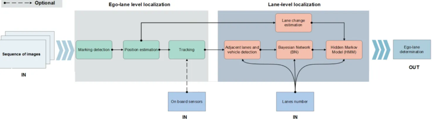
Fig. 1: Overall Algorithm proposed to ego-lane determination that takes in input camera and on board sensors information.
fed with an adjacent lanes detector and lanes number from OSM. Moreover, the proposed network does not depend on the type of sensor and remains modular for other information sources. Hence, we added a vehicle detector to the network. Furthermore, we introduce a Hidden Markov Model to filter the outcome of the Bayesian Network. Compared to [15], no heuristics are made to design the HMM. Thus, we propose a probabilistic formalization for the HMM modeling. At last, we tested our algorithm on two different datasets. First on a collected datasets with two lanes road and which will be available online for other researchers, Second, from some highways images with four lanes road. These datasets are refered in [15].
The remainder of the paper is organized as follows: Section II introduces the problem formulation. Section III describes the ego-lane level localization process. In Section IV we detail the lane-level localization algorithm. Following, Section V presents the real-world experimental results. The paper will be summarized and concluded in Section VI.
II. PROBLEM FORMULATION
As discussed before, we perform the ego-lane determina-tion in sequential fashion as illustrated in Fig 1:
• First, we estimate the lateral position of the ego-vehicle in the lane using camera images in information-driven way.
• Secondly, from the estimated position, we perform the adjacent lanes detection. Depending on the number of lanes, the adjacent lanes are hypothesized and tested. The results of the tested assumption are fed into a Bayesian Network (BN), that takes into account the detector failure rate. Lately, we will show that the proposed BN is modular for other types of detection. • At last, we filter the results using a Hidden Markov
Model (HMM) that takes into account the lane change probability and the accuracy of the detector used. In the following sections, we will discuss the general outline of the algorithm in more details.
III. EGO-LANE LEVEL LOCALIZATION
The ego-lane marking are generally the best seen in the images. Thus, the first step of the overall algorithm consists in the Ego-lane level localization, which is performed by the detection of ego-lane marking.
A. Ego lane-level localization based on a ego-lane-marking detector
In the following, we will briefly explain the method used. The lane-marking detector used is derived from [16], so for more details we invite the reader to look at the complete paper. The different steps of the algorithm are illustrated in Fig 2.
Fig. 2: The different steps of the Ego lane-level localization
The first step of the algorithm is the recognition step, which is based on a recursive recognition driven by a probabilistic model. This model is represented by a vector ud and its co-variance matrix Cud. The vector ud represents the
horizontal coordinates of the left and right ego-lane marking in the image and Cud expresses the confidence interval for
the ego-lane marking in the image as illustrated on Fig 3.
Fig. 3: Confidence intervals for right (in white) and left (in black) edges.
This probabilistic model is defined from a road model X and its co-variance matrix CX. The vector X = (x0, α, Cl, ψ, w)T contains different parameters of the road and the ego-vehicle: x0 being the lateral position of the vehicle relative to the closet lane marking, with 0 being the middle of the ego-lane, α the tilt angle of the camera relative to the road plane, Cl the local curvature of the road, ψ the steer angle of the vehicle and w the lane width of the ego-lane. The recognition of the ego-lane marking is performed in the interval regions defined by the probabilistic model {ud, Cud}. At the end of this step, an estimation of
the vector state ud is made.
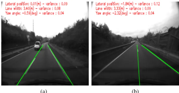
The second step is the localization step, it lies in the esti-mation of the road model {X, CX}, this estimation is directly computed from the estimated image model {ud, Cud}. Fig 4a
shows the results of the ego-lane-marking detection with the estimation of the parameters x0, ψ and L. As the vehicle travels in the middle of lane, the x0 value is equal to 0.01. In Fig 4b, the lateral position estimated is equal to −1.84m as the vehicle changes the lane from the right to the left.
(a) (b)
Fig. 4: Ego-lane marking detection with the corresponding x0, L, ψ estimation.
Finally, the last part of the algorithm is the tracking step, where the aim is to provide a smaller confidence interval for the next image, than the one provided by the initial image model. To do so, we update the model road estimated {X, CX} using a Kalman filter [16], that takes as input the distance traveled by the ego-vehicle between two frame images, which can be retrieved from on board-sensors.
IV. LANE LEVEL LOCALIZATION
Once the ego-lane localization is estimated, we have to perform the lane-level localization in order to correctly choose the right lane on which the vehicle travels. To do so, we propose a probabilistic framework that is split into three stages.
In the first stage, we extrapolate adjacent lanes by as-suming that lanes in the same road have the same width w and same curvature Cl. The second step consists in a Bayesian Network (BN), that takes as input the results of the hypothesized adjacent lane-marking detection, whether these detections succeed or fail. Furthermore, since the proposed BN is modular, we also use an adjacent vehicles detector.
The third step includes a filtering process, using a Hidden Markov Model (HMM).
A. Adjacent lanes extrapolation
The adjacent lanes are extrapolated by taking advantage of the estimated ego-lane localization. Thus, each adjacent lane is described by a probabilistic model {Xl, CXl}, where Xl
contains the parameters (x0, α, Cl, ψ, w)T described in III-A and Cl refers to the corresponding co-variance matrix. Assuming that the curvature and lane width stay constant for all the lanes in the same road. Thereby, the value of the vector Xl remains the same as X, only the value of x0 will be shifted by a (±iw) , with (−i) indicates that the edge is at the right of the ego-lane and (+i) in the left. The number of adjacent lanes extrapolated is equal to the lanes number, which is assumed to be known. Thus, from a perspective view, the hypothesized lanes are shown in Fig 5.
Fig. 5: Perspective view, ego-lane in solid lines and hypoth-esized edges in dotted lines (case two lanes road)
As mentioned before, the model {Xl, CXl} can be
trans-ferred to the model image {ul, Cul}. As a consequence, ul
represents the horizontal pixel of the edges in the image and Cul its interval confidence. In Fig 6, the adjacent lane
regions of interest resulting from the extrapolation are shown on a image. For each adjacent lane marking, the detection is performed and the results are fed into a Bayesian Network (BN).
B. Bayesian network for ego-lane determination
The BN proposed is designed to be flexible and modular for other detection results from any type of sensor, i.e. vehicle detector, guardrail detector. In order to show the flexibility of the BN, we will first use only adjacent lanes detection to determine the ego-lane, then, we will introduce an adjacent vehicle detector based on DeepLearing available in the litterature (YOLO [17]).
The general architecture of the BN used is illustrated in Fig 7. The nodes described are the following:
- Zki: The element i is observable, this element can repre-sents any element of the road scene: {vehicles, lane-marking, traffic signs...},
Fig. 6: Confidence Intervals for adjacent hypothesized edges for a two lanes road. Green represents the estimated edges of the ego-lane and blue illustrates the confidence intervals for adjacent lanes marking.
- Dki: The detection of the element i is successful, - LBN: The lane on which the ego-vehicle is traveling LBN = {l1, ..., ln}, where l1 indicates the leftmost lane and n the lanes number.
Fig. 7: Graphic representation of the general architecture of Bayesian Network used for the ego-lane determination
Depending on the results of the detection, we infer the probability to belong to a lane {l1, l2, ..., ln} as follows:
P (LBN =li) = P (LBN =li|Dk1, Zk1, ..., Dkn, Zkn) (1)
The lane with the highest probability is chosen to be the lane on which the vehicle travels.
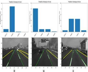
1) Bayesian Network using only adjacent lanes detec-tion (BN+ALD): To start, we only use the adjacent lanes detections as input into our BN. Thus, the ego-lane will be determined considering the result of these detections, whether these success or fail. Fig 8 shows results of the corresponding BN. As illustrated, there are some cases where the BN is unable to overcome the ambiguity to locate the ego-lane. Indeed, this happens when the adjacent edges are not detected or wrongly detected.
2) Bayesian Network with the addition of the adjacent vehicle detector (BN+ALD+AVD): As mentioned before, the BN proposed is aimed to be modular for other detectors. Thus, we use the same BN architecture presented earlier and add the information about the adjacent vehicles.
Fig. 8: Results of ego-lane determination using the BN with only the adjacent lanes detection. In (a) the BN success as the marking are correctly detected, in (b) and (c) the adjacent lanes are not detected, which leads to a false result. In all figures, green represents ego-lane marking and yellow represents adjacent lanes marking detected
The final Bayesian Network used is illustrated on Fig 9, where Dli indicates whether the detection of adjacent lane i is successful. Concerning Dvi, it indicates whether the detection of the adjacent vehicle i is successful. Knowing that this detection is performed in the regions of the image bounded by the neighboring marking-lanes.
Fig. 9: BN with adjacent lanes and vehicles detection (case 4 lanes road)
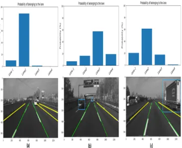
As a result of this addition, the determination of the own-lane is affected as shown on Fig 10.
C. Hidden Markov Model (HMM)
The BN proposed in the section before is applied in a per-frame basis. However, the dynamic relation between two frames is not taken into account. Indeed, the BN does not take into consideration the dynamic constraints of the ego-vehicle (i.e, the ego-ego-vehicle can only change lane to an adjacent lane). In order to take into account these constraints, we filter the output of the BN by a Dynamic Bayesian Network which is the Hidden Markov Model (HMM).
Fig. 10: Results of ego-lane determination using the BN with the adjacent lanes and vehicle detection. For the case (a), the addition of the vehicle detector does not change the result, since no vehicle is detected. However, in (b) and (c) the vehicle detector leads to a correct determination of the ego-lane. In all figures, cyan indicates the bounding box of vehicles detected on the image.
We will use Ltto denote the set of ego-lane state variables at time t, which depends on the lanes number nlanes and which are assumed to be observable. etdenotes the observ-able evidence variobserv-able. The aim of the filter algorithm is to estimate the probability P (Lt+1|e1:t+1). According to [18], this probability can be formulated as follows:
P (Lt+1|e1:t+1) = P (Lt+1|e1:t, et+1)(dividing up the evidence) (2)
= αP (et+1|Lt+1, e1:t)P (Lt+1|et+1)(Baye’s rule) (3)
= αP (et+1|Lt+1)P (Lt+1|et+1)(Markov assumption) (4)
Where α denotes a normalizing constant to make probabili-ties sum equal to 1. By arranging Equation (4):
P (Lt+1|e1:t+1) = αP (et+1|Lt+1) X lt P (Lt+1|Lt, e1:t)P (Lt, e1:t) = αP (et+1|Lt+1) X lt P (Lt+1|Lt)P (Lt, e1:t) (5)
The probability P (et+1|Lt+1) comes from the observation
model. Hence, in this paper from the BN described previ-ously, thus:
P (et+1|Lt+1) = P (LBN) (6)
With regard to the probability P (Lt+1|lt), it comes from
the transition model. It expresses the probability of the ego-lane to change its current state, which is the ego-lane change probability. Finally, the third term P (Lt, e1:t) expresses the
current state distribution. Graphically, we can illustrate the corresponding HMM as in Fig 11.
With the recursive formulation obtained in Equation (5), we can estimate the current ego-lane state given the observa-tion obtained from the BN, but before we have to compute the lane change probability.
Fig. 11: Hidden Markov Model for n lanes case, with L = {l1, l2, ..., ln} being the set of hidden states.
D. Transition probability (Lane change probability) To calculate the lane change probability, we model the lateral position x0 estimated in Section III-A as normal
distribution with meanµx0 and varianceσx0:
x0∼ N (µx0, σ
2
x0) (7)
The valueµx0 and variance σx0 are obtained from the
esti-mated probabilistic model{X, CX}. Therefore, we predict the
lateral positionx0 attk+1 as shown on Fig 12. Accordingly,
the lane-change probability is calculated as follow:
P (Cr) = Z ∞ w/2 1 σx0 √ 2πe −(x−µx0 ) 2 2σ2x0 dx (8) P (Cl) = Z −w/2 −∞ 1 σx0 √ 2πe −(x−µx0 ) 2 2σ2x0 dx (9)
With P (Cr) the probability to right change lane and P (Cl)
the probability to left change lane.
Fig. 12: Lane change probability, with the blue area repre-senting the right change probability.
Now, that we have designed the HMM, we will introduce the real-world experimental results on the following section.
BN + ALD BN + ALD + HM M BN + ALD + AV D BN + ALD + AV D + HM M
2-lanes 91.89% 99.00% 93.60% 99.00%
4-lanes 67.36% 78.36% 74.67% 85.35%
TABLE I: Classification accuracy for ego-lane determination. BN+ALD refers to the BN fed with the adjacent lanes detection, BN+ALD+HMM indicates the HMM with the corresponding BN, BN+ALD+AVD refers to the BN fed with adjacent lanes and vehicles detection and BN+ALD+AVD+HMM refers to the HMM with the corresponding BN.
V. REAL-WORLD EXPERIMENTAL RESULTS
In order to evaluate our proposed method, we tested our algorithm on real driving data-sets. The first one, was collected in the region of Clermont-Ferrand in France, where we drove our vehicle on two lanes road in national highway for a total of 838 frames. Given the number of frames, these datasets were only used to show the effectiveness of the algorithm. In addition, we wanted to compare the performances of our algorithm to the literature on more challenging scenarios. Naturally, we turned our attetion to the KITTI datasets [19]. However, these datasets contain few lanes and few lane-changing scenarios. Thus, we tested our algorithm on some datasets refered in [15] 1. Unfortunately,
all the data were not ready yet. But, we were able to test on some of them, noted as the A4-Highway Italy, for a total of
9528frames. The collected datasets were manually annotated in per-frame basis in order to determine the correct ego-lane classification. In the following, we will refers to our datasets as ”2-lanes” and the A4-Highway Italy as ”4-lanes”.
To show the increment of each component added. We first, determined the ego-lane using only the BN with adjacent lanes. In second instance, we introduced the adjacent vehicles detection in the BN. In all instances, we filtered the outcome of the BN with the HMM. All the results obtained are summarized in Table I.
Considering the results, the increment provided by each module is clearly illustrated. Indeed, in all cases the BN+ALD+AVD provides more accurate classification then the BN+ALD, which suggests that the addition of an another information source will also improve the accuracy obtained. Beside that, in all instances, the HMM improves highly the classification accuracy compared to the outcome of the BN. Which is attributable to the temporal cohesion added in the model, for example, the vehicle can not travel from leftmost lane to rightmost lane in two consecutive frames. Another in-teresting point is the classification accuracy achieved for the 2-lanes datasets. We notice that the accuracy achieved with the BN+ALD+HMM is the same as the one achieved with the BN+ALD+AVD+HMM, which shows that the HMM was sufficiently robust in the first place and the addition of the adjacent vehicles detector did not affect the results.
After investigation on the incorrect results, it appears that the false classifications obtained using the BN+ALD are due to two main reasons: the lane marking are not detected and the lane marking are wrongly detected. For the first case, this can be explained if the lane marking are missing or hidden
1The authors would like to acknowledge the authors of [15] for their help
with the datasets
by an object. For the second case, it shows the limitation of the lane marking detector used. Furthermore, even if the introduction of the adjacent vehicle detection shows excellent results, there are some cases where the vehicle detection are not relevant, for example if the vehicle detected is in the nearby road. To overcome this issue, we will have to determine the localization of the detected vehicle relative to the ego-vehicle, which is not the case since we use only images as input.
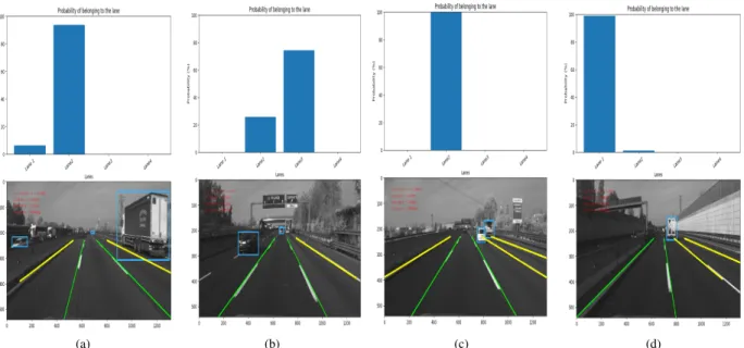
Finally, despite that the author in [15] did not take into account the lane change scenarios and designed empirically the HMM. We manage to outperform his results on the same datasets. Indeed, the author achieved 77%correct classifica-tions, where we were able to reach85.35%on9528frames. In Fig 13 we show ego-lane determination in different example images.
VI. CONCLUSION
In this paper, we tackled the problem of ego-lane de-termination. Unlike other works, we presented a modular Bayesian Network that takes as input different detection results. Moreover, we designed a Hidden Markov Model to filter the outcome of the proposed network. Furthermore, we showed that the proposed algorithm improve lane level localization. In this way, we tested our algorithm on real-world datasets, and we showed the increment provided by each detector.
For our future works, we are currently working on adding detectors from different sensors, i.e., lidar, radar to enhance the proposed framework. In the other hand, we are working on questioning the lanes number information coming from OSM, as we intend to compare it with detection results. Furthermore, we intend to develop a more flexible probabilis-tic framework, which will be able to adapt to lane number change. In addition, we think that improvement can be done on the Bayesian network as the correlation between different detectors are not considered.
Finally, we plan to propose a unique algorithm for all localization parts, that includes road level localization, lane level localization and ego-lane level localization. From a technical point of view, we aim to use our algorithm under ROS [20] for a real-time implementation.
VII. ACKNOWLEDGMENT
This work has been sponsored by Sherpa Engineering and ANRT (Conventions Industrielles de Formation par la Recherche). This work has been sponsored also by the
(a) (b) (c) (d)
Fig. 13: Examples of correct ego-lane determination on the 4-lanes datasets.
French government research program Investissements dav-enir through the RobotEx Equipment of Excellence (ANR-10-EQPX-44) and the IMobS3 Laboratory of Excellence (ANR-10-LABX-16-01), by the European Union through the program Regional competitiveness and employment 2014-2020 (FEDER - AURA region) and by the AURA region.
REFERENCES
[1] N. M. B. Lakhal, L. Adouane, O. Nasri, and J. B. H. Slama, “Risk management for intelligent vehicles based on interval analysis of ttc,” in IFAC Symposium on Intelligent Autonomous Vehicles, Gdansk, Poland, July 2019, pp. 1–6.
[2] D. Iberraken, L. Adouane, and D. Denis, “Multi-level bayesian decision-making for safe and flexible autonomous navigation in high-way environment,” in 2018 IEEE/RSJ International Conference on Intelligent Robots and Systems (IROS), Oct 2018, pp. 3984–3990. [3] ——, “Safe autonomous overtaking maneuver based on inter-vehicular
distance prediction and multi-level bayesian decision-making,” in 2018 21st International Conference on Intelligent Transportation Systems (ITSC), Nov 2018, pp. 3259–3265.
[4] A. Kasmi, D. Denis, R. Aufrere, and R. Chapuis, “Map matching and lanes number estimation with openstreetmap,” in 2018 21st Interna-tional Conference on Intelligent Transportation Systems (ITSC), Nov 2018, pp. 2659–2664.
[5] M. Schreiber, C. Knppel, and U. Franke, “Laneloc: Lane marking based localization using highly accurate maps,” in 2013 IEEE Intelli-gent Vehicles Symposium (IV), June 2013, pp. 449–454.
[6] A. Vu, A. Ramanandan, A. Chen, J. A. Farrell, and M. Barth, “Real-time computer vision/dgps-aided inertial navigation system for lane-level vehicle navigation,” IEEE Transactions on Intelligent Transporta-tion Systems, vol. 13, no. 2, pp. 899–913, June 2012.
[7] V. L. Knoop, P. F. de Bakker, C. C. J. M. Tiberius, and B. van Arem, “Lane determination with gps precise point positioning,” IEEE Transactions on Intelligent Transportation Systems, vol. 18, no. 9, pp. 2503–2513, Sep. 2017.
[8] T.-S. Dao, K. K. Leung, C. M. Clark, and J. P. Huissoon, “Co-operative lane-level positioning using markov localization,” in 2006 IEEE Intelligent Transportation Systems Conference. IEEE, 2006, pp. 1006–1011.
[9] W. Lu, E. Seignez, F. S. A. Rodriguez, and R. Reynaud, “Lane marking based vehicle localization using particle filter and multi-kernel estimation,” in 2014 13th International Conference on Control Automation Robotics Vision (ICARCV), Dec 2014, pp. 601–606.
[10] V. Popescu, R. Danescu, and S. Nedevschi, “On-road position es-timation by probabilistic integration of visual cues,” in 2012 IEEE Intelligent Vehicles Symposium, June 2012, pp. 583–589.
[11] V. Popescu, M. Bace, and S. Nedevschi, “Lane identification and ego-vehicle accurate global positioning in intersections,” in 2011 IEEE Intelligent Vehicles Symposium (IV), June 2011, pp. 870–875. [12] M. Nieto, L. Salgado, F. Jaureguizar, and J. Arrospide, “Robust
multiple lane road modeling based on perspective analysis,” in 2008 15th IEEE International Conference on Image Processing, Oct 2008, pp. 2396–2399.
[13] D. Svensson and J. Srstedt, “Ego lane estimation using vehicle observations and map information,” in 2016 IEEE Intelligent Vehicles Symposium (IV), June 2016, pp. 909–914.
[14] T. Gao and H. Aghajan, “Self lane assignment using egocentric smart mobile camera for intelligent gps navigation,” in 2009 IEEE Computer Society Conference on Computer Vision and Pattern Recognition Workshops. IEEE, 2009, pp. 57–62.
[15] A. L. Ballardini, D. Cattaneo, R. Izquierdo, I. Parra, M. A. Sotelo, and D. G. Sorrenti, “Ego-lane estimation by modeling lanes and sensor failures,” in 2017 IEEE 20th International Conference on Intelligent Transportation Systems (ITSC), Oct 2017, pp. 1–7.
[16] R. Aufr`ere, R. Chapuis, and F. Chausse, “A model-driven approach for real-time road recognition,” Machine Vision and Applications, vol. 13, no. 2, pp. 95–107, Nov 2001. [Online]. Available: https://doi.org/10.1007/PL00013275
[17] J. Redmon and A. Farhadi, “Yolov3: An incremental improvement,” arXiv preprint arXiv:1804.02767, 2018.
[18] S. J. Russell and P. Norvig, “Artificial intelligence (a modern ap-proach),” 2010.
[19] A. Geiger, P. Lenz, C. Stiller, and R. Urtasun, “Vision meets robotics: The kitti dataset,” The International Journal of Robotics Research, vol. 32, no. 11, pp. 1231–1237, 2013.
[20] M. Quigley, K. Conley, B. Gerkey, J. Faust, T. Foote, J. Leibs, R. Wheeler, and A. Y. Ng, “Ros: an open-source robot operating system,” in ICRA workshop on open source software, vol. 3, no. 3.2. Kobe, Japan, 2009, p. 5.