Design of a slurry layer forming station and improved fluid handling system for raster processes in 3DP®

Design of a Slurry Layer Forming Station and Improved

Fluid Handling System for Raster Processes in

3Dp™

by

David C. Ables

A.B., Harvard University (1995)

Submitted to the Department of Mechanical Engineering

in partial fulfillment of the requirements for the degree of

Master of Science in Mechanical Engineering

at the

MASSACHUSETTS INSTITUTE OF TECHNOLOGY

May 2001

[:rv ',.-'

.c.

\1

©

Massachusetts Institute of Technology 2001. All rights reserved.

Author ...

..

Department of Mechanical Engineering

May 11, 2001

(

~

Certified by ... " ... , ... _ ... _ ... .

Emanuel M. Sachs

Professor of Mechanical Engineering

Thesis Supervisor

Accepted by ...

... .-.-. ... .

Ain 1. Son in

Chairman, Department Committee on Graduate Students

Design of a Slurry Layer Forming Station and Improved Fluid Handling

System for Raster Processes in

by

David C. Ables

Submitted to the Department of Mechanical Engineering on May 11, 2001, in partial fulfillment of the

requirements for the degree of

Master of Science in Mechanical Engineering

Abstract

Three-Dimensional Printing (3DPTM) is a rapid-manufacturing process originally developed at MIT for building parts directly from CAD-generated models. Parts are fabricated in "slices" by creating a complete layer of powder and then selectively joining powder particles with a polymer binder deposited using a moving printhead. Traditional 3DPTmbuilds layers

by spreading dry powder and prints binder using a rastering scheme with a continuous-jet

printhead. For smaller parts and greater accuracy, a variation on the process called slurry

3DPTM (s3DPTM) uses raster-built slurry layers and a vector-printing scheme with a drop on demand (DoD) printhead. This here thesis presents efforts to improve core technology

in both dry-powder 3DPTmand slurry 3DPTM.

One of the most critical steps in s3DPTMis the building of the slurry layers. To avoid intra- and interlayer defects the slurry layer must be rastered at high deposition rates to promote line merging and better layer quality. The difficulty lies in the design of a machine capable of oscillating the slurry nozzle at the required frequencies. Fortunately, such a design was completed and the machine built as part of a collaborative effort with TDK Japan to build an s3DPTMmachine for manufacturing small parts. The design uses a reciprocating countermass strategy to recycle mechanical energy and eliminate troublesome vibrations. A general overview of this slurry layer forming station (LFS) is given, along with an in-depth treatment of several components, including the forcers, centering system, and interface software.

And speaking of rastering, dry-powder 3DPTmrelies on this strategy for printing binder, just as the LFS uses a raster method to build powder layers. Beginning with observations made during the design of the LFS, the fluid-handling system was redesigned to improve binder droplet stream stability during the carriage traverse and turnaround. The improve-ment was made possible by repositioning a smaller version of the "Clamshell" constant pressure vessel used to set the fluid flow rate to the printhead carriage itself and using a closed-loop control system to maintain a constant fluid level in the Clamshell. Draw-ings, parts lists, schematic diagrams, and assembly instructions are included for building additional fluid control systems.

Thesis Supervisor: Emanuel M. Sachs Title: Professor of Mechanical Engineering

Acknowledgments

Acknowledgements are traditionally where we thank all of the people who supported us through the trying times of the academic, er, paradise that is graduate school at MIT. We try to sound humble and deferential, when the truth is we all would rather try to pass off everything as completely our own sweat and inspiration. How do you think we got here in the first place?

I should start by thanking my family for their support and encouragement over the past few years. However, my family hasn't understood a single thing I have done since I was in the 8th grade, but I suppose I shouldn't let that bother me. And they never hesitated to remind me how nice the weather was in the Texas Hill Country during the snow, rain, sleet, and icy wind of Boston winters, which I really appreciate. But they were my biggest cheering section, and the moral support for everything happening outside of school is certainly why I'm getting out of here at all, so I thank you profusely.

I should also thank Antoine, D'Andre, Tonisha, Alex, Stanley, Alma, Vanessa, Darrin, Tiffanye, and all of my other former students from Calvin Simmons Middle School in Oak-land, CA. If you hadn't made my life so miserable for two years then graduate school might have actually seemed difficult and stressful.

Angie, some might question your inclusion here, but no hard feelings, and I couldn't have come here and made it through the first year without you. Good luck in all that you do.

Steven Calcote, Jason Waterman, and Grant Taylor helped keep me inspired and mo-tivated with visions of leaving graduate school to go start the next billion-dollar Internet company. Maybe someday, guys...

And then there are the many members of the 3DPT"lab without whom I would have just had to lie and make-up everything in this godforsaken thesis:

Ben Polito, possibly the smartest kid I ever met. I'd better hear about your becoming a faculty member within 10 years or you're toast. Students need people like you.

Jim Serdy, whose patience, kindness, experience, and willingness to help were exceeded only by his appetite. Thanks for taking on my myriad questions and problems as your own, and thanks for the use of your van.

Chris Stratton, Kris Seluga, Patrick Petri, Hiro Tsuchiya, Yasushi Enokido, and every-one else involved with the TDK machine design. Never have so many come together to make such a mess that ultimately worked. It was a fun ride, guys.

Julie Baars Kaczynski, Heather Lee, and Liev Aleo, who helped me spend lots of MIT's money on cool toys and who answered all of my annoying questions.

And all of the other people who remained in and around the lab: Adam, Vinay, Dave, Diana, Diane, David, Ram, Renee, Markus, Andreas, Scott, Rich, Sherry, Michael, and everyone else. You were more than just extras, even though you were paid the same.

Oh yeah, and what's-his-name. Ely Sachs: sage, mentor, and taskmaster; who shared his inspiring outlook on academia, continually demonstrated new and creative problem solving methods, guided all of this work, and somehow resisted the urge to ever put my head through a wall. It goes without saying that I couldn't have done it without you.

And lastly, let me thank the good people at Toscanini's. If I miss nothing else from Boston I will miss your coffee.

Contents

I Preamble 14

1 Introduction to Everything 15

1.1 The 3DPTMProcess ... ... 15

1.1.1 How Does it W ork? . . . . . . . . . . . . . . . . . . . . . . . . . . . 15

1.1.2 W hat is it Good For? . . . . 16

1.1.3 Slurry 3DPTIv. Dry Powder 3DPTM. ... ... 17

1.1.4 Vector v. Raster Printing . . . . 17

1.2 The Slurry Layer Forming Station . . . . 18

1.3 The Raster Fluid Handling System . . . . 18

II The Slurry Layer Forming Station 20 2 Introducing the LFS 21 2.1 Slurry Layers are Hard to Make ... 21

2.2 Where Others Have Tread . . . . 21

3 Functional Overview 23 3.1 D esign Overview . . . . 25

3.2 Slow A xis . . . . 27

3.3 C arriage . . . . 28

3.3.1 Baby Clam shell . . . . 28

3.3.2 G alvanom eter . . . . 29

3.3.3 Carriage Linear Motor . . . . 31

3.4.1 Countermass Linear Motor 3.4.2 Centering System . . . . 3.5 Software . . . . 3.5.1 PMAC Code . . . . 3.5.2 Driver API . . . . 3.5.3 TDK Program . . . . 4 The Linear Motors

4.1 Background . . . . 4.1.1 How a Linear Motor Works 4.1.2 Commercial Options . 4.1.3 Design Metrics . . . . 4.2 D esign . . . . 4.2.1 Geometry . . . . 4.2.2 Field Assemblies . . . . 4.2.3 Armatures . . . . 4.3 Conclusion . . . . 5 The 5.1 5.2 Centering Mechanism Design ... Results ... 6 Control Software 6.1 Driver API ... 6.2 PMAC Software ... 7 LFS: Conclusion

III The Raster Printing Fluid System

8 Introducing the Mini Clam Shell

8.1 O ld System . . . .

8.2 Some Theory ... ...

8.3 Motivation for Improvement ...

32 32 33 34 35 35 37 37 37 40 41 44 44 45 49 54 56 56 57 59 60 61 64 65 66 66 66 69 . . . . . . . . . . . . . . . . . . . . . . . .

8.4 New System . . . .6

9 The Pump 71 9.1 Requirements ... ... 71

9.2 Evaluation of Options ... ... 71

9.2.1 Direct Control of Masterflex Drive . . . . 72

9.2.2 Direct Control of Gearmotor . . . . 72

9.2.3 Programmable Masterflex Pump . . . . 73

9.3 R esults . . . . 73

10 The Sensor 75 10.1 Description and Characterization . . . . 75

10.2 Modulated Driver Design . . . . 76

10.2.1 Concept . . . . 77 10.2.2 D river . . . . 80 10.2.3 Isolator . . . . 82 10.2.4 Demodulator . . . . 82 10.2.5 F ilter . . . . 83 10.3 R esults . . . . 84 11 Itsy-Bitsy Clamshell 86 11.1 Membrane . . . . 87

11.1.1 Modeling the Membrane . . . . 87

11.1.2 Membrane Design . . . . 90

11.2 Clamshell Geometry . . . . 95

11.2.1 Air and Fluid Pockets . . . . 95

11.2.2 Membrane Seal . . . . 95 11.2.3 Inlet/Outlet Holes . . . . 96 11.2.4 Sensor Mount . . . . 97 11.2.5 Viewing Windows . . . . 97 11.2.6 Summary . . . . 98 11.3 Air Reservoir . . . . 99

11.3.1 Compressible Gas Theory . . . . 99 69

11.3.2 Air Reservoir Design . . . .

12 The Controller

12.1 Theory . . . . 12.2 Analog Design . . . .

12.2.1 Sensor Scaling and Display 12.2.2 Proportional Controller . .

12.3 Electronics Summary . . . .

13 Overall System

13.0.1 Common Disturbances .

13.0.2 Results Summary . . . .

14 Fluid System: Conclusion

IV Conclusion

15 Tying it All Together

V Appendix

A Carriage Motor HOWTO A. 1 Armature ...

A.1.1 Materials List ...

A.1.2 Drawings ...

A.1.3 Process Plan ...

A.2 Field Assembly ... A.2.1 Materials List ...

A.2.2 Drawings ...

A.2.3 Process Plan ... B Countermass Motor HOWTO

B. 1 Armature ... B.1.1 Materials List ... . . . . . . . . . . . . . . . . . . . . . . . . . . . . 99 101 101 102 102 104 105 107 107 111 113 114 115 117 118 118 119 120 120 126 126 128 128 136 136 137 . . . . . . . .

B.1.2 Drawings ... ... 138 B.1.3 Process Plan . . . . 139 B.2 Field Assembly . . . . 145 B.2.1 Materials List . . . . 146 B.2.2 Drawings . . . . 147 B.2.3 Process Plan . . . . 147 B.3 Centering Assembly . . . . 148 B.3.1 Parts List . . . . 149 B.3.2 Drawings . . . . 150 B.3.3 Process Plan . . . . 150

C LFS Driver Software HOWTO 165 C.1 PMAC Program . . . . 166

C.2 W indows Driver API . . . . 166

C.2.1 Overview . . . . 166

C.2.2 Function Overview . . . . 167

C.2.3 Settings File: MITCTRL.INI . . . . 173

C.3 Modifications . . . . 174

D Raster Fluid System HOWTO 175 D.1 Parts Lists . . . . 176

D.1.1 Pump Parts . . . . 176

D.1.2 Control Electronics Parts . . . . 176

D.1.3 Clamshell Parts . . . . 178

D.1.4 Reservoir Parts . . . . 178

D.2 Assembling the System ... ... 178

D.2.1 Making the Reservoir . . . . 179

D.2.2 Making the Clamshell . . . . 180

D.3 Making the Control Electronics . . . . 181

D.4 System Manual . . . . 181

D.4.1 Calibration . . . . 182

D.4.2 Startup Procedure . . . . 182

List of Figures

1-1 The 3DPTMProcess Illustrated. . . . . 16

1-2 The s3DPTMProcess Illustrated . . . . 17

1-3 Vector Printing versus Raster Printing . . . . 18

2-1 Rastered Slurry Layers with and without Line Merging . . . . 22

3-1 The TDK/MIT Slurry Printer . . . . 23

3-2 TDK/MIT Slurry Printer Layout . . . . 24

3-3 Rastering a Slurry Bed . . . . 25

3-4 Carriage Countermass Oscillation System . . . . 26

3-5 The Slurry Layer Forming Station . . . . 27

3-6 Zig-zag Lines Formed by Stationary Nozzle . . . . 28

3-7 The Nozzle Carriage and all its Toys . . . . 29

3-8 The "Baby" Clamshell . . . . 30

3-9 The Galvanometer and Nozzle Arm . . . . 30

3-10 Unidirectional Bed Formation . . . . 31

3-11 Registered versus Unregistered Layers . . . . 32

3-12 Bidirectional Bed Formation . . . . 33

3-13 The Carriage Linear Motor (View from Beneath) . . . . 34

3-14 The Countermass . . . . 35

3-15 The Countermass Linear Motor . . . . 36

4-1 How a Motor Works . . . . 38

4-2 Rotary Motor Schematic . . . . 39

4-3 Schematic of Non-Commutated Linear Motor . . . . 39

4-5 4-6 4-7 4-8 4-9 4-10 4-11 4-12 4-13 4-14 4-15 4-16 5-1 5-2

6-1 The Layered Interface Design for the LFS Software . . .

6-2 Organization of the PMAC PLC Code . . . .

8-1 Schematic of Old Clamshell Style System . . . .

8-2 Pressure Pulses Arise When the Carriage Turns Around

8-3 Schematic of New Fluid System . . . . How to Hook Up and Kill an Op-Amp . .

Building a Pump from a Small Gearmotor Remote Control of a Masterflex Pump . . The IR LED Photosensor ...

Sensor Response for Different Membranes Sample Function

f(t)

Modulated Signal

f(t)

Demodulated Offset Signal m*(t) . . . . .

Icky Force Ripple in Commercial Linear Motor . . . . The Carriage Linear Motor . . . . The Countermass Linear Motor . . . . Solid Model Rendering of the Carriage Motor Magnet Rail . . . . . Field Uniformity of Carriage Magnet Rail . . . . Countermass Motor Field Assembly (Top Half Removed) . . . . .

Countermass Motor Field Assembly (Top Half Shown) . . . . Field Uniformity of Countermass Magnet Assembly . . . . Carriage Motor Armature Design . . . . Solid Model Rendering of Finished Carriage Motor Armature . . . Countermass Motor Armature Design . . . . Solid Model Rendering of Finished Countermass Motor Armature . Repelling Force v. Distance for Magnets . . . . The Countermass Centering Assembly . . . .

41 44 45 47 48 49 50 51 51 53 53 54 57 58 . . . . 59 . . . . 62 67 68 70 9-1 9-2 9-3 10-1 10-2 10-3 10-4 10-5 10-6 10-7 . . . . 7 2 . . . . 7 2 . . . . 7 3 . . . . 7 6 . . . . 7 6 . . . . 7 7 . . . . 7 8 . . . . 7 8 . . . . 7 9 . . . . 7 9

10-8 Filtered Modulated Signal with Offset Removed . . . 10-9 Block Diagram of Sensor Circuit . . . .

10-10Schematic of LED Driver . . . .

10-11Schematic of Inverting Isolation Amplifier . . . . 10-12Schematic of AD630 Demodulator Chip . . . . 10-13Schematic of Butterworth Filter . . . . 10-14Response of Modulated v. DC Sensor Configuration

11-1 11-2 11-3 11-4 11-5 11-6

Basic Clamshell Design . . . .

Membrane Used in Model Derivation . . . . Membrane Pressure Drop v. Deflection . . . . Sensor Response for Wet and Dry Membranes . . . . Undesirable Critical Points for Highly Reflective Membranes Red Silicone Membrane Abraded and Unabraded Response

11-7 Membrane Compression Boss Detail . . . . 11-8 Front Exploded View of the Clamshell . . . . 11-9 Rear View of the Clamshell . . . .

11-10Air Reservoir Location on Alpha Machine . . . . 12-1 First Order Control Model of System . . . . 12-2 Sensor Signal Conditioning and Display Circuit . . . .

12-3 Proportional Control Circuit . . . .

12-4 Complete Control Circuit Schematic . . . .

13-1 System Response for Drained Clamshell . . . . 13-2 System Response for Leak . . . . 13-3 System Response for Change in Air Pressure . . . .

13-4 System Response for Clog . . . .

13-5 Off-Board Clamshell Streams During Turnaround . . . . 13-6 Mini-Clamshell Streams During Thrnaround . . . .

A-1 The Carriage Linear Motor (Previously Shown as Figure 4-6) A-2 Solid Model Rendering of Finished Carriage Motor Armature A-3 Solid Model Rendering of Carriage Motor Field Assembly . .

86 87 90 92 93 94 96 98 98 100 102 103 104 106 . . . . 108 . . . . 109 . . . . 110 . .. .. . 111 . . . . 112 . . . . 112 119 121 127 . . . . 80 . . . . 81 . . . . 81 . . . . 82 . . . . 83 . . . . 84 . . . . 85

B-1 The Countermass Linear Motor (Previously Shown as Figure 4-7) . . . . 137

B-2 Solid Model Rendering of Finished Countermass Motor Armature . . . . 139

B-3 Solid Model Rendering of Countermass Motor Field Assembly . . . . 146

B-4 The Countermass Linear Motor (Previously Shown as Figure 5-2) . . . . 149

B-5 Countermass Centering System Assembly . . . . 150

C-1 The Layered Interface Design for the LFS Software . . . . 165

C-2 Organization of the PMAC PLC Code . . . . 166

D-1 Schematic of Fluid System (Reprint of Figure 8-3) . . . . 175

D-2 Air Reservoir Schematic & Location on Alpha Machine . . . . 179

D-3 Assembly Diagram for the Clamshell . . . . 180

D-4 Front Exploded View of the Clamshell . . . . 180

D-5 Rear View of the Clamshell . . . . 181

List of Tables

4.1 M agnet Properties . . . . 4.2 Carriage Motor Armature Design Specifications . . . . 4.3 Countermass Motor Armature Design Specifications . . . . 6.1 The Functions in the LFS Driver API . . . .

11.1 Clamshell Membrane Characteristics . . . .

A.1 A.2 A.3 A.4 B.1 B.2 B.3 B.4 B.5 D.1 D.2 D.3 D.4

Materials List for Carriage Motor Armature . . . . Process Plan for the Carriage Motor Armature . . . . Materials List for Carriage Motor Field Assembly . . . . . Process Plan for the Carriage Motor Field Assembly . . .

Materials List for Countermass Motor Armature . . . . . Process Plan for the Countermass Motor Armature . . . .

Materials List for Countermass Motor Field Assembly . . Process Plan for the Countermass Motor Field Assembly . Materials List for Countermass Centering Assembly . . .

Materials List for Fluid System Pump . . . . Materials List for Fluid Control Electronics . . . . Materials List for Fluid Clamshell . . . . Materials List for Air Reservoir . . . .

46 52 52 60 94 . . . . 119 . . . . 121 . . . . 127 . . . . 128 . . 137 . . 140 146 . 147 149 176 176 178 178

Part I

Chapter 1

Introduction to Everything

1.1

The 3DP

Process

In the never-ending saga of life imitating Star Rek, efforts have intensified over the past few decades in trying to build parts directly from computer models. 3D Printing (3DPTM), a processes developed at MIT in the early 1980s, is one such solid freeform fabrication process that holds several advantages in terms of geometric and material flexibility.

1.1.1 How Does it Work?

The 3DPTMprocess is an additive process that builds up a part layer by layer based on a

CAD file that has been "sliced" using post-processing software. The following process is

then repeated for each slice:

1. Spread powder to provide material.

2. Print binder to define geometry of slice.

3. Dry binder (if necessary).

4. Drop piston to make room for next layer.

This process, illustrated in Figure 1-1, culminates in our part held together by the binder encased in a block of dry powder. The excess powder is removed to produce a green part skeleton that is not at full density. We can then improve the strength and density of the part by either sintering in a furnace or by infiltrating with another substance.

Spread Powder Print Selected Area Lower Piston Layer

Last Layer Printed Completed Parts

Figure 1-1: The 3DPTM_{Process Illustrated}

1.1.2 What is it Good For?

There are two primary advantages to 3DPTM: First, since a complete powder layer is always spread, the unprinted powder can support complicated overhangs and other geometries. Second, the process works for any material available in powder form so long as a suitable binder can be identified. 3DPTMtechnology has been applied to a number of different classes of parts, both at MIT and by commercial licensees working with MIT.

" Model Prototyping

* Metal Parts

" Injection Molding Dies " Machining Tooling

" Timed-Release Drugs " Ceramic Parts

" Electronic Components

* Medical Prosthetics

1.1.3

Slurry 3DP

"v. Dry Powder 3DP

In order to achieve better resolution in printed parts we must print with finer powder. However, we run into physical limits for submicron-sized powder, where van der Waals and electrostatic forces prevent us from dry-spreading effectively. For small, fine-featured parts we instead use slurry processing to form our layers, suspending our particles in a slurry and building a wet layer which we then dry to provide dry powder in which to print binder. This extra step means s3DPTlis slower than dry powder-based 3DPTM, so we generally only use this method for printing very small, fine-featured parts.

X-Y Positioning System

Heating T- Heating

Sluny 4 Binder iet

i.

ffioW

Shurry Deposition Drying Powder Bed Printing Binder Diying Binder

Repeat Cye Printed Object Printed Powder Bed _mill Porous Substrate

Finished Part Redisper Unbod _{Powder Bed} Retrieved Part

Figure 1-2: The s3DPTMProcess Illustrated

The complete s3DPT~process is illustrated in Figure 1-2. Note that it is now more difficult to extract our green part since we must redisperse the unbound powder. s3DPTlis generally used for printing ceramic parts.

1.1.4 Vector v. Raster Printing

Slurry layers are an improvement over dry powder layers in terms of thickness and particle size, but we also would like to improve the resolution of the binder printing step. For this, we use vector printing instead of raster printing. Vector printing is to raster printing as old ink pen plotters are to modern inkjet printers. Vector printing, as illustrated in Figure 1-3, first draws the outline of the part before filling it in using raster methods. This initial outline step improves the surface finish of the part.

X axis X axis (Fast axis)'O

Vector printing Rmster printing

Figure 1-3: Vector Printing versus Raster Printing

1.2

The Slurry Layer Forming Station

The most fundamental piece of an s3DPT"Machine is the Layer Forming Station (LFS), since all subsequent steps depend on having a layer of slurry on which to print. The

LFS described here was designed and built as part of a collaborative effort with the TDK

Corporation of Japan to build a slurry-based 3D Printer.

The LFS is a complicated piece of machinery and the result of the efforts of a talented team of people. This thesis being submitted for my degree, it is most appropriate if I focus on the portions of the LFS for which I was directly responsible, rather than trying to grab credit for everyone else's work.

However, some sort of context for the overall LFS machinery is necessary, so I will provide a brief overview of all of the different subsystems comprising the machine, followed

by in-depth treatments of the elements I designed, namely the linear drives, the centering

mechanism, and the software interface. Part II of this thesis deals with my efforts in this arena.

1.3

The Raster Fluid Handling System

Any 3DPT~process involves much moving around of fluids. The particular problem of jetting slurry from a moving nozzle during layer formation brought to light some issues in fluid handling that were also found to exist in more traditional powder-based 3DPT"as part of raster printing the binder. This somewhat tenuous bridge connects Part II with Part III, which details the design of an enhanced fluid-handling system for use with binder

in raster-based 3DPTM.

The main text will deal with the theory, design process, and results for the new system, and detailed plans for constructing additional systems are included in the Appendix.

Part II

Chapter 2

Introducing the LFS

The process for forming slurry layers is at the core of s3DPTM. Unfortunately, it is quite a bit more complicated than spreading dry powder. Fortunately, previous efforts have lead

to a recommended approach which is encapsulated in the LFS design for the MIT/TDK

machine [4, 11].

2.1

Slurry Layers are Hard to Make

In order to print binder to form a 3DP part we must first have a layer of powder on which to

print. When a layer is built from a slurry this process becomes more complicated than simply

spreading out dry powder at the desired thickness. Instead, the slurry must be deposited

and then the liquid removed to leave only the dry powder ready to receive the binder. The

liquid is removed via the process of slipeasting, where the liquid is absorbed into a porous

substrate (which may include previously slipcast layers), in a manner similar to soaking up

water with a sponge. The trick is getting the liquid to slipcast without producing bubbles, cracks, or other defects in the slurry layer whilst simultaneously creating a flat layer. This

is the fundamental problem the LFS attempts to solve.

2.2

Where Others Have Tread

One obvious scheme for forming layers of a reliable thickness from a fluid would be to

spin-coat the substrate, as is done in photodeveloping and microelectronic fabrication [3].

Another method might be to spread a layer in a single strip using tape casting. This method has been investigated, but layers formed in this fashion contained far too many defects to be usable in the 3DPT process [11].

Work by DeBear and Saxton [4, 11, 5] found that the most effective means for building slurry layers was to raster the layer, one line at a time, using a single nozzle on a moving carriage. This lead to the development of the infamous "bicycle wheel" apparatus [11, 4].

While rastered slurry layers met the criterion of a low percentage of defects, the overall layer quality was not particularly good due to the preservation of individual slurry lines in the final layer. The solution to this problem is then to deposit slurry lines fast enough that they can merge and eliminate the ridges resulting from depositing completely slipcast lines next to one another. Under this approach, the slurry lines must be deposited faster than

Conventional Layer Deposition

(Lines remain discrete, leading to defects)

Rapid Line Deposition

(Lines merge while wet, improving finish and reducing defects)

Figure 2-1: Rastered Slurry Layers with and without Line Merging

the wet front can advance. Results using this method as tested on the LFS described here have proven to be quite successful [9].

Chapter 3

Functional Overview

The TDK/MIT Slurry-based 3DPrinter (Figure 3-1) was built as part of a collaborative effort between the MIT 3DPT~lab and the Mechatronics Division of TDK Japan. MIT was responsible for developing the Layer Forming Station and the Printhead, while TDK designed the overall software and hardware platform that integrated the various processing stations together into the overall printer.

Figure 3-1: The TDK/MIT Slurry Printer

The printer itself consists of 4 stations, illustrated in Figure 3-2:

" Layer Forming

* Layer Height Measurement

e Binder Printing

Layer height Binder printing measurement station K4-Binder handling unit XY table for printhead DoD printhead (8 nozzles) Powder bed I

\

Figure 3-2: TDK/MIT Slurry Printer Layout

The Layer Forming Station (LFS) is described in this chapter. The Convective Drying station, ironically enough, blows heated air on the powderbed to dry the new slurry layer or freshly printed binder. The Layer Height Measurement station is used to obtain accu-rate measurements of the layer thickness for eventual feedback control of Layer Forming parameters. The Binder Printing station is an x-y table with 8 DOD printheads that uses a vector printing scheme.

To actually print a part, the movable powderbed is shuttled along a linear stage among the 4 stations in the following order to make-up a single cycle which is repeated layer by layer until the part is finished.1 A print cycle looks like

1. Layer Forming,

2. Slurry Drying,

3. Height Measurement,

'This takes approximately a million hours. Several efforts are currently underway to speed up this process. Slurry handling unit Nozzle & Nozzle Arm Powder bed

1

Rn

LEL

4. Binder Printing, and

5. Binder Drying.

This chapter focuses on the Layer Forming Station, first describing the LFS as a whole and then briefly discussing the components critical to its operation that were the focus of my efforts. The LFS builds layers by rastering them out one line at a time onto a moving substrate. The combination of flyover speed of the slurry nozzle, slurry flow rate, and substrate traverse speed determines the resulting layer height. In addition, the nozzle speed and substrate speed are chosen so that the wetting front will promote line merging before slipcasting occurs.

3.1

Design Overview

In a nutshell, the LFS builds layers by oscillating the slurry nozzle back and forth along the y-direction.2 In the meantime, the substrate moves along at a constant velocity in the

x-direction. The resulting slurry lines then scan along to form a layer which then slipcasts to form a dry powder layer.

Figure 3-3: Rastering a Slurry Bed

2

It takes a rather large nut to provide a shell big enough to hold our machine.

-Achieving the necessary speeds of 1.5 m/s and interarrival times of < 0.3 ms on a 2 kg carriage requires massive accelerations during turnarounds. These types of accelerations would potentially melt any electromechanical system asked to accelerate such a mass in such fashion [13], in addition to shaking the heck out of the machine. Clearly, a more clever mechanical method is needed.

After the success of the bicycle wheel [4, 11, 5], a new scheme was developed that also uses recycled mechanical energy to accelerate the carriage. In this system, a large, reciprocating countermass collides with a lighter carriage. If the countermass is sufficiently larger than the carriage, then the collision will just reverse the velocities of each body with a low change in momentum, resulting in minimal vibration of the unit. Careful design can assure minimal energy loss during the collision, which can be most efficiently be done by pumping the energy back into the countermass due to its lower velocity and kinetic energy.

Forcer

Cam age moves at high speed while Counterm ass

moves slowly in opposite direction

Spnng

Nozzle Cariage .At) 0

Carriage and Countermas s

collide; zero net

momentum transfer

Velocities reverse and energy is restored to Counterm ass via forcer

Figure 3-4: Carriage Countermass Oscillation System

" Substrate Axis ("Slow Axis")

" Carriage

" Countermass

e

These will be briefly described in more detail below.

Countermass Forcer

Umbilical with electrical and slurry connections

Counterm ass Air Bearings

Figure 3-5: The Slurry Layer Forming Station

3.2

Slow Axis

As was mentioned above, layers are formed using a raster process with a nozzle moving back and forth. With the velocities and accelerations needed for the nozzle carriage, it is easier to move the substrate beneath the carriage. The substrate upon which the powderbed is built rides on a linear stage, which is generally referred to as the "Slow Axis" due to its not-so-blinding speed.

In order to achieve ideal bed quality we want the slurry rastered as parallel lines for uniform thickness across the bed. However, due to the high speed of the nozzle and narrow

line spacing, it is not possible to move the substrate in a step-like fashion, so instead it is moved at constant velocity. This has the unfortunate fact that the slurry lines are formed in a zig-zag pattern, while parallel lines are obviously preferable in terms of bed quality.

Fist (NOZzle CaniMge) A"s M0tion

L ines

Path

Stow (Substrate) Axis Motion

Figure 3-6: Zig-zag Lines Formed by Stationary Nozzle

The linear stage selected includes a linear optical encoder capable of resolving to 0.1 Am, which allows for very precise and reliable control of the Slow Axis speed. To compensate for the fact that the slurry lines aren't parallel the nozzle is actually maneuvered using a laser-scanning Galvanometer, described below in Section 3.3.2, in order to produce parallel lines.

3.3

Carriage

The Carriage is the heart of the LFS, it being the part that actually jets the slurry to the substrate below, and it is shown in all its splendor in Figure 3-7. The carriage rides on air bearings for low friction and contains a number of components to allow for accurate control over the nozzle position, slurry flow, and carriage velocity and position.

3.3.1 Baby Clamshell

The "Clamshell" is a staple of 3DPTMmachines, used to deliver fluids at a constant flow rate by maintaining a specified pressure in said fluid. The Clamshell maintains a constant pressure in the fluid in order to provide a constant flow rate. Since a rather large portion of this thesis is dedicated to the art and science of clamshells, I will skip the thorough

ex-- I .,.-,, - .- ~---- - -- -- ~---- -

-Galvonometer

(Buried under wires) Galvonometer Camr age

\Controller

Encoder

W.Umbilic al

Carri age

Air Bearings Carriage Pressure Vessel

Figure 3-7: The Nozzle Carriage and all its Toys

planation until Part III. Traditionally the Clamshell is located away from the carriage, the pressurized fluid being delivered by an umbilical cable. However, this standard approach was found to yield poorly formed slurry beds, and the Clamshell was reduced in size (hence the affectionate name "Baby Clamshell") and placed on board the carriage to keep the fluid pressure constant at delivery. This change in design formed the basis for more exten-sive work redesigning the binder fluid system for raster-based 3DPTM, which is discussed in excruciating detail in Part III. For now I'll stipulate that the presence of the Clamshell elim-inates troublesome pressure pulses in the fluid lines due to the high accelerations produced in the carriage turnaround.

3.3.2 Galvanometer

The slurry nozzle is attached to an arm whose angle with the y-axis can be precisely controlled. There are two different schemes, then, for straightening the slurry lines. The first, known as unidirectional forming, involves switching the nozzle back and forth so that

Slurry Purge Outlet _{Air Inlet}

slurry

IW et Level Sensor

Mount

Wet (Slurry) Hal Dry (Air) Half

Slurry Outlet (Not Visible)

Figure 3-8: The "Baby" Clamshell Galvonometer

Nozzle

Carrig _Nozzle

Mtr Ann

Figure 3-9: The Galvanometer and Nozzle Arm

two beds are formed simultaneously, one using positive-y passes and one using negative-y

passes. This method also allows the flexibility of placing the lines with precise registration

between layers, as indicated below, as well as compensating for any error in the Slow Axis

position. The limitation under this scheme is that the beds cannot be wider than a maximum

limit determined by the range of motion of the Galvanometer arm.

The bidirectional forming scheme uses both positive- and negative y-passes. While the

interarrival times along the slurry lines will no longer be constant, this method allows for the formation of larger beds. This method is dependent on the motion controller's ability to update the Galvanometer position often enough to keep the lines straight. It is also limited

t Nozzle Path Slow' (subdndae) Axis Motion

Figure 3-10: Unidirectional Bed Formation

of Slow Axis position error.

3.3.3 Carriage Linear Motor

A small linear forcer is used on the Carriage for the purposes of starting up the LFS and positioning the Carriage when the station is not in use. The motor also gives the option,

not currently utilized, of actively maintaining a constant velocity over the powderbed. A

linear encoder is used to determine the carriage position and velocity, used by the PMAC

motion controller (see Section 3.5.1). The design and performance of this Linear Motor is

detailed in Chapter 4.

3.4

Countermass

The Countermass fulfills the dual purpose of (1) providing the energy input to the system to

keep the nozzle moving and (2) minimizing the change in momentum during the turnarounds

of the carriage so that there is a minimum amount of vibration transmitted to the overall printer. It consists of two stainless steel rails riding on air bearings for low friction, two large stainless steel blocks with springs for the carriage collision, and the linear forcer that drives the system. Its mass is approximately 10 times that of the carriage.

Figure 3-11: Registered versus Unregistered Layers

3.4.1 Countermass Linear Motor

A non-commutated Linear Motor similar in concept to the Carriage Forcer (Section 3.3.3

is used to drive the Countermass. Since no commutation is needed, supplying the needed force output from the motor is accomplished simply by reversing the current through the motor armature when the Carriage changes direction. There is no direct feedback for the position or velocity of the countermass, although some proportional control is done based on the Carriage velocity. The design and performance of this Linear motor is detailed in Chapter 4.

3.4.2 Centering System

Since the force on the Countermass must reverse with each collision with the Carriage, some mechanism is needed to keep the center of mass for the system from drifting and the resulting error from crashing everything into the bearing blocks. (This is generally

Nozzle Arm Must Continually

Adjust Over Powder Bed to Keep Lines Straight While

Slow Axis is Moving

_A

1-Y

Nozzle Path

Figure 3-12: Bidirectional Bed Formation

an undesirable thing.) The necessary restoring force is provided by 3 magnets, 2 fixed and one moving magnet attached to the Countermass. The polarities are set so that both fixed magnets repel the moving magnet-the (small) resultant force is sufficient to make the center of mass behave. A slight damping force is applied to the Countermass by attaching an aluminum sheet to the armature coil. The resulting Eddy Currents caused by moving the aluminum in the magnetic field assembly produce enough damping force to keep the system stable.

This particular system is discussed in more detail in Chapter 5.

3.5

Software

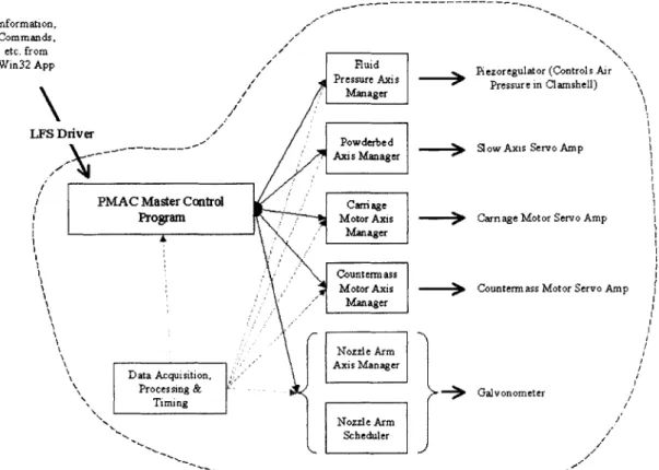
Something has to make all of these motors and things go, and that thing for the LFS is an 8-axis PMAC motion control board. All of the necessary brainpower for operating the LFS resides on the PMAC, which then uses a driver library to interface between the PMAC and the overall control software for the printer.

Underside

of Carriage

Coil

Magnets

Magnet Rail

Figure 3-13: The Carriage Linear Motor (View from Beneath)

3.5.1

PMAC Code

As was mentioned before, there are a total of 8 available axes on the PMAC motion control board. Five of them are utilized for the LFS:

" Slow (Powderbed) Axis

" Countermass Motor

" Carriage Motor

" Nozzle Arm

" Air Pressure

The PMAC offers two different methods for controlling each axis: motion control pro-grams or PLC propro-grams. Motion Controls are suitable when a normal-flavored motor is connected in a servo loop configuration. In our case, only the Slow Axis can be controlled in this manner. All other axes are controlled using custom PLC code. A master scheduling PLC manages all of the different axes.

Linear Motor Springs

Spring Blocks

Rails

Figure 3-14: The Countermass

3.5.2 Driver API

While the PMAC can put the LFS through its paces, so to speak, something has to tell it

which pace is currently appropriate.3 A driver API is defined for the LFS that communicates

with the PMAC by sending ASCII commands over the ISA bus, into which the PMAC is plugged. This allows for a clean split of responsibilities, allowing changes to be made to the inner workings of the LFS software while still maintaining compatibility with the main

control software.

3.5.3 TDK Program

The entire printer is controlled by a Windows Win32-style Application on a computer running Windows 98. Users interact with the software via both standard keyboard/mouse inputs and a touch-screen interface. This main control software is responsible for managing the overall print process, which includes scheduling and operating the different stations, interpreting the slice data and generating vector paths, and a very long laundry list of

other tasks needed for printing to go, er, smoothly.

3

Coil

Mount Ann

Coil Leads

Magnet

Assembly

Coil

(Not Visible)

Chapter 4

The Linear Motors

In order to make the LFS do the shake-and-bake required to raster-build a layer, something has to actually make the nozzle carriage move back and forth. I was anointed with the task of making this happen, either through selecting an appropriate commercial solution or constructing a custom design. Since the Carriage and Countermass are not directly coupled, two different forcers would be needed. This chapter describes the design of both of these critical components, work which took place between August 1999 and March 2000.

4.1

Background

Before diving into "How I spent my first semester graduate school," some brief information on the initial efforts is in order, including some of the theory behind what makes a motor mote.

4.1.1 How a Linear Motor Works

The existence of electric motors stems from the simple equation describing the force F on a conductor of length 1 carrying current I through a magnetic field of strength B:

F = BIl (4.1)

with the direction of the force given via the right hand rule between the magnetic field and electric current [7].

North Magnetic Pole

Magnetic Field

B

Current I

South Magnetic Pole

Active Length I

Figure 4-1: How a Motor Works

Rotary Motors Since current must travel in a loop, one problem in motor design is configuring the magnetic field so that the force on the wire carrying the current "in" does not cancel out the force on the wire carrying the current "out." A typical solution, shown in Figure 4-2, uses opposite-poled magnets on two halves of the motor. In order to maintain the proper alignment of current and magnetic field, a brush commutator is used to "swap" the current as the conductor rotates through the transition between magnetic fields.

Non-Commutated Linear Motors A linear motor in its simplest form is just an

"un-wrapped" rotary motor. "Non-commutated" means that the force remains constant in di-rection for constant current. Two possible configurations for non-commutated linear motors are shown in Figure 4-3.

In Configuration A, only one leg of the coil is used to generate force, so the motor is not very efficient. The travel of the motor is theoretically unlimited, but since we need to catch all of the magnetic flux lines in the rail for maximum efficiency, we end up needing a larger and larger rail, which eventually becomes a problem as we start to saturate the metal. Another problem is that the constant magnetic field produces a bending moment in the magnet rail, and a longer travel and therefore magnetic rail equals a larger deflection,

Armature

Norh

Pol 4

-F

.;Commutator

Figure 4-2: Rotary Motor Schematic

Configuration A: "Unlimited" Motion bib, Norh Nrt Active Area Configuration B: Limited Motion rth South Range of Motion

Figure 4-3: Schematic of Non-Commutated Linear Motor

which can be bad.

Configuration B uses two legs of the coil, but since we get constant force for current in one direction, we can't run the coil past the edge of the magnetic area or we will suddenly have the force reverse itself.

Commutated Linear Motors If we want Configuration B to have a larger travel dis-tance we must change the current as we get to the oppositely-aligned set of magnets. This is the principle behind commutated linear motors, as shown in Figure 4-4. It uses two legs of the current loop, so it is more efficient. The armature coil is shown in two different

Active Area

Active Area

South North South North South North

Figure 4-4: Schematic of Commutated Linear Motor

positions. Note that due to the different alignment of the magnets, opposite current flow is needed to produce the same force vector. Commercial linear motors will generally consist of multiple phases, where each phase is a separate current loop offset so that the force remains constant as the coil moves among the different magnet pairs. In Figure 4-4, connecting both of the coils to the same carriage would produce a two-phase motor.

Unlike a rotary motor, where commutation can be done using a constant current supply and a mechanical method such as brushes, linear commutation generally requires a varying current supply to each phase to eliminate force ripple. Multiple phase sinusoidal commu-tation is a rather high-maintenance scheme, requiring a sophisticated amplifier and linear encoder.1

Since the magnets are oriented in opposing pairs, the rail does not have to form a continuous loop, meaning the travel is only limited by the length of the magnet rail. An additional advantage of the commutated configuration is that no bending moment is exerted on the magnet rail since alternating magnet pairs are of opposite polarity and each pair cancels out another.

4.1.2 Commercial Options

Commercially available linear motors require a necessarily complicated scheme involving a linear encoder and motion controller to perform the necessary commutation. In an effort to buy something off the shelf that would be relatively simple to operate we evaluated a

3-phase linear motor available from Aerotech that used Hall Effect sensors to detect the switched-polarity magnet pairs rather than a precise linear encoder. The amplifier itself then switched phase polarity appropriately. Unfortunately, the limited resolution of the commutated drive current (imagine a 2-bit encoded sine wave) produced a very noticeable step-like force ripple in the motor, shown in Figure 4-5.

14.0 -13.8 13.6 -- . -13.4 13.2 -S13.0 12.8 12.6 -12.4 ... 12.2 -12.0 0.00 1.00 2.00 3.00 4.00 5.00 6.00 Position [in.]

Figure 4-5: Icky Force Ripple in Commercial Linear Motor

Such behavior is inherent to the design of such self-commutating motors, so our next option was to examine the difficulty in designing and fabricating our own motors.

4.1.3 Design Metrics

The number of available geometries for a non-commutated linear motor are somewhat lim-ited due to the fact that current must travel in a loop, meaning that for at least part of the loop, the geometry must be designed to either change the magnetic field over different legs of the loop or portions of the loop must remain outside of the magnetic field. The latter approach was used for the Carriage motor, while the former was used for the Countermass. When designing the motor, we are concerned with how to achieve maximum force under the constraints of available power and heat dissipation. Our power is limited both by what

we can achieve with a reasonable servo amplifier and by what the wire can handle before melting. Heat dissipation is more of a concern under an impulse, namely can we apply peak forces with the motor without the entire thing turning into a molten mess?

Motor Efficiency To first examine the relationship between force and power, we take note of the following key relations for force, power, and resistance.

F = BInl (4.2)

P = I2R (4.3)

PRL

R A (4.4)

A

where F is the force output, B is the magnetic field strength, I is the current in the wire, n is the number of turns, 1 is the "active" length of wire subject to the magnetic field,

R is the resistance of the wire, PR is the resistivity of the wire, L is the total wire length,

and A is the cross sectional area of the wire.

If we then define the following terms

A* = nA (4.5)

l = H (4.6)

L = nH (4.7)

where A* is the total conductive cross sectional area, H is the length of a single winding, and q is the active length fraction, we find the following equation for the power input to the motor:

P = F2PR (4.8)

(Brq)21A*

Our design metric for Force v. Power is then

F2 = (Br7)211A* (4.9)

P PR

turns of our wire. However, the total conductive cross sectional area A* depends on the packing density of the wire. The ideal scenario would be one turn of a large conductor that fit the required space completely, but this is impractical from a design and manufacturing standpoint, so smaller, 24 AWG wire was chosen since it was easy to work with and would pack densely.

Impulse and Heat Dissipation The change in temperature for power input of a fixed duration depends on the following formulae:

AT = q (4.10)

mc

q = Pt (4.11)

m = LAPD (4.12)

where AT is the rise in temperature, q is the energy input, m is the mass of the wire, c is the specific heat capacity of the wire, PD is the density of the wire, and t is the duration of the impulse.

The rise in temperature is then given by

AT = F2tPR(4.13)

(BTUHA*)2 _pDc

so that the design metric for impulse heat dissipation is given by

F2t (Bq1UA*)2_pDc

(4.14)

AT PR

Here we can conclude that we want to maximize our conductor volume, IIA*, which then provides the biggest heat sink. In practical terms, we want to maximize the packing density of our windings. This is why encapsulating the coil in epoxy is done-it fills in the air gaps and increases our bulk thermal mass while also improving thermal conductivity.

The end result of maximizing these design measures is that we want lots of turns of "reasonably" fine gauge wire. The driving factor becomes finding a wire gauge that's easy to work with so that we can pack our turns as tight as possible. In both cases we want to maximize our active fraction q and subject as much of the conductor as possible to the magnetic field. This is subject to geometric constraints, however.

4.2

Design

After deducing all of the important considerations in designing a motor (which were largely intuitive, but it's always good to have centuries of physics to back up our ideas) we actually had to design and build them.

4.2.1 Geometry

Much of the design of the motors was mandated by the geometrical constraints of the ma-chine. The Carriage motor needed to be small and light with a long stroke (see Configuration

A from Figure 4-3). The Countermass motor had a short stroke and little space constraint,

so its design measures could be maximized with less constraint, as in Configuration B from Figure 4-3.

Carriage The Carriage motor configuration is shown in Figure 4-6. The armature is a

Magnets

I \VI

Armature Coil Contacts

Magnetic Flux Lines

Nozzle Caniage

Figure 4-6: The Carriage Linear Motor

square loop with one leg of the magnet rail running through its center axis. Only one leg of the coil is then used to actually provide the force, making the motor less efficient. In order to have a return path for the magnetic flux the magnet rail must form a loop, which limits

the total stroke of the motor.

Countermass The Countermass motor configuration is shown in Figure 4-7. It uses a

Armature Coil

Magnets

Magnetic Flux Lines

Magnets

Figure 4-7: The Countermass Linear Motor

square loop for the armature coil with two of the legs subject to the magnetic field. The stroke of the motor is then limited by the coil size, since the opposite legs must have opposing field directions. It would be rather disastrous if one leg of the coil found its way into the wrong field area since the direction of force would suddenly be reversed. This can

be prevented via mechanical constraints, and the necessarily smaller stroke is acceptable in this case since the Countermass stroke need only be about 3 cm.

4.2.2

Field Assemblies

A field assembly must form a loop in which the magnetic flux can travel. Low carbon steel was used as the magnetic conductor with size chosen so as to allow for minimal field leakage and nickel-plated to prevent rust.2 _{The magnets were of a special blend developed} 2Since the possibility exists of working with ferrous slurries, it would be very bad to have the slurry being jetted in the presence of a strong magnetic field, which would at best affect the flow and layer quality and

by Crumax, chosen for its high field strength, available size configurations, and resistance

to corrosion.

Shape 1 in. Square

Thickness 0.25 in.

Material CrumaxTM Model D40727

Magnetic Field at 0.25 in. 0.15 T

Table 4.1: Magnet Properties

Each field assembly was also designed with threads for jacking screws so that the oppos-ing halves of the magnet loop could be more easily separated and joined. The magnets are extremely strong, and it is very difficult to align the field assembly pieces and even more difficult to separate them without a little help.

Carriage The Carriage needed a long stroke and had minimal space available for the motor. The field assembly was therefore designed as a long, thin loop. One side-effect was that only single magnets could be used rather than pairs, which provide double the field strength. The constraint was maximizing the stroke with minimum field leakage. Since the motor and field assembly were right next to the carriage this was of definite importance.

One concern was deflection of the flux return bar under the distributed load caused by the attractive force of all of the magnets. If we model the rail as a simply supported beam 300mm long with square cross section of 30mm x 30mm, then the maximum deflection at the midpoint is given by Equation 4.15.

5w L4

J = 384 _384EI (4.15)

Here w is the distributed load, found to be 736 N/m, L is the span length of 300mm, E is the Elastic Modulus (190 GPa), and I is the moment of inertia, which is 6.75 x 10-8m4 .

Under these conditions the maximum deflection J was calculated to be 0.01 mm, which is actually a conservative overestimate since our actual rail is supported more rigidly than a simply-supported beam and will thus have even less deflection.

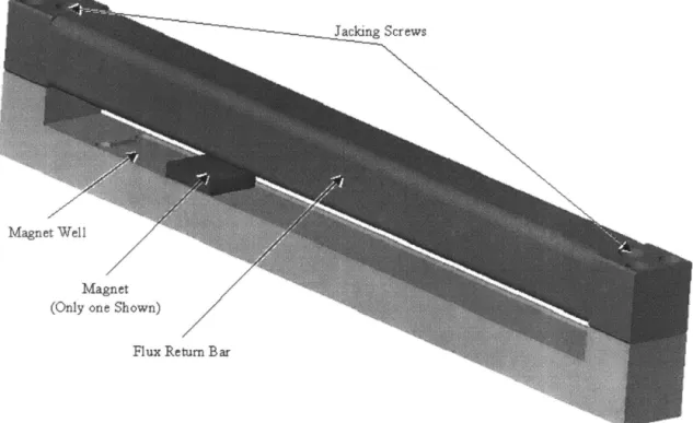
A solid model of the magnet rail is shown in Figure 4-8. The flux return bar has radiused

Magnet Well

Magnet (Only one Shown)

Flux Return Bar

Figure 4-8: Solid Model Rendering of the Carriage Motor Magnet Rail

larger and thus reduce magnetic field line leakage. The opposite end of the field assembly loop has a slight well machined in order to keep the magnets in place. This is necessary

because while we want a minimal gap between the magnets to improve field uniformity, the

magnets themselves will naturally move to maximize this distance since they are all aligned with the same polarity.

The average field strength of the magnet rail was measured to be 0.39 T (a = 0.02) with field uniformity as shown in Figure 4-9.

Countermass Since the Countermass had little in the way of space constraints and only

needed a short stroke, more care could be taken in maximizing its efficiency. The field assembly was then designed to create opposing magnetic fields over opposite legs of a square coil. This way half of the winding perimeter can be utilized to produce force.

Figure 4-10 shows the field assembly for the Countermass motor with the top and one side removed for easier viewing. Two magnet wells are visible, although magnets are only shown in one. All four magnets in each well are of identical polarity, but the front well is

0.5 0.45 0.4 0.35 0.3 T 0.25 S 0.2 * 0.15 0.1 0.05 0 50 100 150 200 Position [mm]

Figure 4-9: Field Uniformity of Carriage Magnet Rail

reversed from the back well since they act on opposite sides of the armature coil. The gap between the magnets visible in the front magnet well is needed because the magnets are simply too strong to fit into a group of 4 without being extremely unstable. Since the wire in the armature coil spans across the magnet well, this gap will not cause any variance in the force. Holders for the centering system magnets (See Chapter 5) are also visible on the bottom of the field assembly.

The top half of the field assembly, visible in Figure 4-11, is identical to the bottom half with the magnet polarities reversed. Having the magnets configured in opposing pairs doubles the strength of the magnetic field. The top and bottom plates which hold the magnets are machined from low-carbon steel, which is good for directing magnetic field lines. The side spacers also act as the mounting pieces that attach the field assembly to the rest of the LFS. The spacers are machined from Aluminum, which is not ferrous, thus focusing the magnetic field more intensely in the field assembly. Field lines were shown previously in Figure 4-7.

The magnets were oriented in pairs to produce an average field strength of 0.5 T. Field uniformity is shown in Figure 4-12. The gap between the magnets is clearly visible, but field is symmetric about this point, so we can still expect solid response from the motor.

-.

...

..

-.

...

.

--

---