Defining and Detecting Churn in Truckload Transportation

(1)

Defining and Detecting Churn in Truckload Transportation by

Saad Bin Rehan

Master of Science in Operations Analytics and Management Worcester Polytechnic Institute, Worcester Massachusetts

and

Kawin Jungsakulrujirek

Bachelor of Science in Engineering (Mechatronics Engineering) Asian Institute of Technology, Bangkok Thailand

Submitted to the Program in Supply Chain Management in Partial Fulfillment of the Requirements for the Degree of

Master of Applied Science in Supply Chain Management at the

Massachusetts Institute of Technology

June 2021

The authors hereby grant to MIT permission to reproduce and to distribute publicly paper and electronic

copies of this capstone document in whole or in part in any medium now known or hereafter created.

(2)

Signature of Author: ______________________________________________________ Department of Supply Chain Management

May 14, 2021

Signature of Author: ______________________________________________________ Department of Supply Chain Management

May 14, 2021

Certified by: ____________________________________________________________ Dr. Chris Caplice Executive Director, Center of Transportation and Logistics Capstone Advisor

Accepted by: ____________________________________________________________ Prof. Yossi Sheffi Director, Center for Transportation and Logistics Elisha Gray II Professor of Engineering Systems Professor, Civil and Environmental Engineering

(3)

Defining and Detecting Churn in the Truckload Transportation Industry by

Saad Bin Rehan and

Kawin Jungsakulrujirek

Submitted to the Program in Supply Chain Management on May 14, 2021 in Partial Fulfillment of the

Requirements for the Degree of Master of Applied Science in Supply Chain Management

ABSTRACT

The truckload transportation industry is an established industry, in the US, with annual revenue for for-hire truckload reaching greater than 300 billion dollars in 2019. A major problem encountered by for-hire truckload carriers is a sudden, unexpected and sustained reduction in shipment volume over lanes referred to as ‘churn’. Churn leads to a significant problem in the balance in the carrier’s network which, in turn, drives up costs, reduces revenue and decreases driver satisfaction. In this capstone, which is a firstofitskind study within the truckload industry, we leverage data from our sponsor -a l-arge n-ation-al trucking firm - to form-ally define churn using three p-ar-ameters: b-ase, drop and duration. Based on this definition we identify churn by origin within the carrier’s network and then establish correlations between the characteristics of an origin and the likelihood of churn at that origin. This framework allows carriers to quickly detect churn before it materializes and take proactive steps to mitigate its negative impact. Our research on churn opens up avenues for further study in this area, within the TL industry, including studying churn at a larger scale to develop more widely applicable ways of defining, identifying and detecting churn.

Capstone Advisor: Dr. Chris Caplice

(4)

ACKNOWLEDGEMENTS

Throughout the undertaking of this capstone project, we have received a great deal of support, encouragement and guidance.

We, first, want to thank our advisor Dr. Chris Caplice whose expertise was invaluable at every step of this project. His insightful and thorough feedback was instrumental in helping us bring our work to a higher level. He was sincerely committed and invested in making this capstone a success and we are lucky to have worked under his able guidance and thoughtful leadership.

This project would not have been made possible without the guidance, and experience of senior management of our sponsor company. They were always extremely cooperative and kind, and were willing to share insights and ensure a quick turnaround of data to facilitate the completion of this capstone.

We also want to express our sincere gratitude to Pamela Siska, from MIT’s Writing, Rhetoric and Professional Communication department. Her multiple rounds of feedback and corrections helped make our thesis a coherent, grammatically correct version of itself. She was incredibly patient and kind throughout the process.

We also want to extend a note of thanks to Arsalan Akhter, a close friend, who took it upon himself to answer all our silly questions and provide valuable input on our writing to help improve the flow and structure of the capstone.

On a personal note, we want to thank our families - our parents, for always being our biggest advocates. I (Kawin) want to specially thank Kanit, my brother, for his words of encouragement. I (Saad) want to thank my partner in crime for life, Amna, for being the biggest critic of my work, an unwavering source of support, and pushing me to be the best version of myself, every day. Last, but certainly not the least, we would also like to give a shout out to Ayrah (Saad’s daughter) whose beautiful smile kept us going when things became too crazy.

(5)

1 - Introduction

Truckload transportation is an established industry in the United States with total revenue reaching 680.4 billion dollars in 2019. The total revenue of the full truckload -for-hire component was estimated to be greater than 300 billion dollars (31st Annual Council of Supply Chain Management Professionals (CSCMP) State of Logistics Report).

The for-hire trucking transportation industry is divided into 2 segments: TL (truckload shipping) and LTL (less than truckload shipping). TL refers to the transport of freight that goes directly from the point of origin to destination. LTL shipping, on the other hand, moves smaller quantities from multiple origins to multiple destinations by consolidating and routing through multiple terminals. Our sponsor is a for-hire TL carrier and this capstone pertains specifically to the TL industry.

The truckload shipping process primarily consists of three players that each have a distinct role (Caplice, 2007). First, there are shippers: companies that are the suppliers or owners of goods shipped. Second, there are carriers: these are trucking companies that transport the goods. Traditionally, these companies own the transportation assets including equipment and resources like trucks, trailers and drivers. Their primary role is the movement of freight. Third, there are receivers: which are firms to which shipments are sent.

To haul freight across road networks through carriers, most shippers typically run an annual RFP (request for proposal) process. Shippers initiate the process by generating and distributing an RFP that contains the details of the shipping operation including

(10)

expected volume, lanes (origin and destination pairs), lead time etc. The RFP is distributed to both incumbent and new potential carriers that then respond with a bid. The shipper ranks the bids in order of most to least attractive. The factors considered by the shippers include price, historical on time performance, expertise and experience of the carrier. The shipper then chooses one or more primary carrier(s) in each lane and enters into an annual contract with the carrier. This contract is binding in price, but not in volume supplied by the shipper or capacity supplied by the carrier.

1.1 Importance of Balance in a Carrier’s Network

Contracts between a shipper and carrier improve the predictability for both parties by locking in the shipment rate charged by the carrier for the length of the contract. However, as noted above, volume and capacity are not guaranteed. There is often a high degree of variability in shipment volumes which puts a TL carrier in a vulnerable position.

Truckload carriers are a direct form of transportation. This means that a large portion of the carrier’s cost is driven by the search and movement cost of looking for and capturing a follow-on load (Caplice, 2007). TL carriers are subject to a high degree of economies of scope. The chance of securing a follow-on shipment out of the destination of the prior load directly impacts the cost of hauling the next load. By creating a balanced network (having consistent freight lanes), carriers are able to drive down the unpredictability associated with connection costs. This, in turn, lowers their overall costs. This is why carriers prefer consistent shipment volumes across their network. It also allows carriers to better plan which lanes to cover and how to price them. A sudden loss

(11)

in volume over a lane can create an imbalance which adds costs for finding a new load, hence making business less profitable. The existence of consistent freight lanes also allow carriers to build long term relationships with the shippers. These advantages are lost when carriers suddenly and unexpectedly lose volume from a shipper on a given lane. It impacts the costs to serve multiple other lanes, not just the direct lane.

The sudden reduction in shipment volume on a lane can happen due to two main reasons. First, the shipment volume for a lane never materialized. This can happen for a number of reasons including shifting demand, changing networks etc. Second, the shipper might decide to use a different carrier that may be offering a more competitive price. Both of these factors can result in churn in the carrier’s network. A carrier cannot determine which of these two cases is responsible for the sudden loss in volume; the volume simply stops. Variability in load volume on a lane or out of an origin is expected. However, a sustained drop in volume over a lane or out of an origin causes balance problems. This phenomenon of sudden, unforeseen and sustained loss of business is referred to as churn.

1.2 Churn

In TL, churn is loosely defined as a sudden, dramatic, and unplanned decrease in volume tendered from a shipper lasting for a sustained duration. As explained above, churn impacts the balance in a TL carrier’s network. The movement of a truck without paying load is referred to as ‘empty miles’ or ‘deadhead’. Churn in a carrier’s network can increase the level of empty miles required to reposition drivers and trucks. This, in turn, will drive costs up, reduce revenue, and decrease driver satisfaction, which can

(12)

impact driver retention. This is why quickly detecting churn in a carrier’s network is important. In this capstone project, we formally provide a more specific and nuanced definition of churn and then apply this definition to identify churn in a for-hire, full truckload carrier’s network. We also develop a method to quickly detect churn so that proactive steps can be taken to minimize it.

Based on our definition of churn, we then identify churn in the carrier’s network. Our next step is to look for correlations between churn and the characteristics of the origin region of the shipment. Our hypothesis is that churn will be dependent on some of these origin level characteristics (as described in Chapter 3). If our hypothesis is correct, we will use those variables to detect when churn would occur at an origin and develop a real-time churn detection model for our carrier. With this capstone, we aim to fill the gap in churn detection in the truckload transportation industry by delineating a framework and tools needed to detect churn. The impact that accurate detection of churn can have for our carriers can be robust and can help them run their businesses in a more efficient and profitable way.

The remainder of this report is organized as follows. Chapter 2 discusses the prior research done on churn across different industries and identifies gaps. Chapter 3 formally and precisely defines churn within the truckload transportation industry. Using this definition, churn is identified within our data set. Chapter 4 presents the algorithm developed to rapidly detect churn in a carrier’s network. Different methods and approaches are presented and results are discussed. Finally, in Chapter 5, we summarize our findings, offer recommendations, and make suggestions for further research in this area.

(13)

2 - Literature Review

In this chapter we review previous research conducted on customer churn prediction (CCP). Because no research on CCP has been done on truckload transportation, we review the CCP literature of other industries, including banking, telecommunications, and gaming, three industries where CCP is most commonly studied (Kilimci et al, 2020). In these industries, churn is defined as the situation where a customer stops doing business with a company, such as when a subscriber cancels their subscription (Amin et al., 2018, Kilimci et al. 2020, Amornvetchayakul and Phumchusri, 2020).

2.1 Past Research

A stream of literature pertinent to CCP focuses on businesses with enriched data settings. Do et al. (2017) predicted customer churn experienced by an internet service provider. The industry saw 2% of churn on a monthly basis. De Caigny et al. (2018) presents CCP in 14 datasets across the banking, telecom, energy and retail industries. They used a hybrid combination of logistic regression and decision trees to predict churn defined as a consumer dropping the service completely. The combination of models showed significant improvement over using logistic regression or decision tree alone. Interestingly, random forests outperformed the combination of the two methods in this study (De Caigny et al., 2018). Singh et al. (2018) also studied churn in the telecom industry comparing random forests with other classical classification methods, such as support vector machine (SVM), logistic regression, and k-nearest neighbor (k-NN). The study analyzed a sensitivity analysis in the various ratios of churning to non-churning

(14)

customers, randomly sampled from the dataset. Random forests consistently yielded the highest accuracy in all the methods selected.

Figalist et al. (2020) proposed a study of CCP in business-to-business (B2B) context in the telecom industry. In 2020, researchers had still not allocated much attention to B2B’s CCP because of its lower data availability in customer samples (Figalist et al., 2020). However, unlike business-to-customer (B2C), B2B businesses have fewer customers with much higher transactional values, making churn detection very important for them.

2.2 Feature Selections and PCA

These studies used a wide variety of available data features (or customer characteristics) in their models. Do et al. (2017) aggregated 121 features for the internet provider industry to predict churn into 3 categories of data: customer information, customer data usage, and customer service information. Figalist et al. (2020) used 50 features, classifying them as being either static and dynamic, and applied principal component analysis (PCA) to reduce this to 25 features. PCA was also used by Simion et al. (2018), who reduced the number of features from 168 to 42. Kilimci et al. (2020) introduced a CCP analysis of sentiment data, data in English-sentence structure, from Appstore and Google Play to predict the cancellation of service in the gaming industry. User reviews were used as the features in this study, providing more insights in gaming CCP. Deep learning for text reading was later used to support this analysis. Table 1 lists the different sets of features used in the literature.

(15)

Table 1: Summary of the Past Literature

Author Industry Churning Service Feature Feature no. Monthly Churn Rate Alvarez et al. (2013) Food Weekly Subscription Not Described Not Described 27%

Do et al. (2017) Internet Provider Monthly Internet Package Customer info, usage,_service 121 2%

De Caigny et al. (2018) Banking, Telecom,_{Energy, Retail} Not Described 14 Databases Ranging between_{16 and 303} Not Described

Simion-Constantinescu et

al. (2018) Retail Pharmaceutical Purchase

Customer info and transactions

168 → 42

using PCA 27%

Singh et al. (2018) Telecom Telephone Service Package Customer info and_usage 20 14%

Amin et al. (2018) Telecom Telephone Service Package 4 Databases Ranging between_{21 and 100} 15%

Figalist et al. (2020) B2B Software Software Subscription Customer info and_usage _{using PCA}50 → 25 Not Described

Kilimci et al. (2020) Gaming User Activity Sentiment Analysisfrom Appstore and

Google Play Not Described Not Described Amornvetchayakul and

Phumchusri (2020) Software Software Subscription

Customer usages and

(16)

All of these studies use features of data prior to the churn actually happening. There is a gap to using data features within the churning period if the transactional data is available to potentially improve the accuracy of CCP. In this capstone, the concept of using real-time information, within potential churn periods, to improve the real-time accuracy of CCP will be referred to as the detection model.

2.3 Monthly Churn Rate and Churn Definition

Industries differ in their monthly churn rate, that is the percentage of customers who leave or cancel their subscription. Industries such as software or gaming have a very high churn rate, as high as 50% monthly (Amornvetchayakul and Phumchusri, 2020). Telecommunication has a slightly lower rate, at about 14-15% (Singh et al 2018, Amin et al. 2018). Internet service has the lowest churn rate, 2% per month, yet still finds CCP to be very important in customer retention (Do et al., 2017). Having a very low churn rate can lead to a problem in setting up an objective function for the accuracy of classification methods. Synthetic Minority Oversampling Technique (SMOTE) is a well-known method for dealing with cases with a low churn rate (Do et al., 2017; Singh et al., 2018; Amin et al., 2018). SMOTE is a data pre-processing technique that generates samples of data whose dependent variable is on a minority group. Instead of making a copy of them which would lead to overfitting, SMOTE generates new unique data that could be used in the analysis. Studies on the telecommunication and internet service usually use SMOTE to deal with this dataset imbalance. Table 1 presents the churn ratios from studies of different industries.

(17)

Most of the literature found on the industries mentioned above has defined churn as a 100% reduction in customer demand for products or services for a specific duration ranging from 16 days to 12 months. Ullah et al. (2018) defined churn as an account termination or 180 days of inactive transactional activities in banking. Do et al. (2017) used 16 days as the signal for discontinuation of service subscription for internet services. Simion-Constantinescu et al. (2018) defined churn as customers who did not make a transaction for the past 12-month in Pharmaceutical products. In 2013, a Harvard study case about Lufa Farm also introduced a churn concept and used 28 day-duration as the indicator for the unsubscription in service (Alvarez et al., 2013).

2.4 Voluntary and Involuntary Churn

Amin et al. (2018) presented a distinction between two types of customer churn: voluntary and involuntary. Voluntary customer churn is where the customer decides to cancel their service subscription. Involuntary churn, on the other hand, is where the provider dismisses the customer. For the purpose of retaining customers, voluntary customer churns should be clearly segmented to improve the CCP analysis of customer churn an organization is looking to reduce. The study then categorized and studied CCP only for the voluntary customer churn (Amin et al., 2018). In our study, we were not able to classify churn into voluntary and involuntary segments. Singh et al. (2018) also discussed the concepts of voluntary and involuntary customer churn, but used different wording: active (voluntary) and passive (involuntary) churn.

In our capstone, the differentiation between voluntary and involuntary churn is not able to be studied due to the lack of information in our data set. The information of when the carrier rejects tenders from a shipper is not in the dataset provided, but is

(18)

known to the sponsor company. Because voluntary and involuntary customer churn has different root causes for its occurrences, additional information of the churn status on customer dismissals would definitely open a wider analysis of CCP.

2.5 Prediction Methods

Churn is typically defined by a binary variable; the customer does or does not cancel the service. This lends itself to being modeled as a “classification problem”. Many classification algorithms have been studied in past CCP analyses. The most common algorithms are:

1. Decision Tree - A classification model classifying binary/discrete data in a tree format. It is popularly used as the first basic model to explain classification algorithms.

2. Logistic Regression - A binary regression model that is transformed from linear regression.

3. Support Vector Machine (SVM) - A classification model that uses multiple lines and/or curves to separate data into a binary/discrete output.

4. k-Nearest Neighbour (k-NN) - A classification model that uses a number of training data (k counts) closest in features to determine the predicted one.

5. Random Forest - An advanced classification algorithm combining multiple decision trees to improve their ability to predict output binary/discrete variables. 6. Deep Neural Network - An advanced algorithm that can also be used both for

classifications. The algorithm is well-known for the ability to replace all mathematical functions. The algorithm mimics the application of human brains with neuron layers in its computation.

Recent studies have concluded that random forest is the most accurate in predicting churn (Singh et al., 2018; Amornvetchayakul et al., 2020). Alternative methods available are k-Means, local outlier factors (LOF), and cluster-based local

(19)

outliers factors (CBLOF) (Ullah et al, 2019). In this capstone project, a decision tree model will be implemented. We have chosen a decision tree because it works well on small datasets and the results are easy to interpret.

2.6 Detection Model

In section 2.2, the concept of using real-time information within the churning period to improve CCP’s accuracy was defined as the detection process. We found no studies using the detection model in CCP research but it was implemented in one similar study. Tripathy (2020) used the duration of the real-time drop of customer demand to predict the possibility of phantom inventory. Phantom inventory is defined as a situation where the inventory system suggests the availability of inventory when it is not actually there. The probability of this phantom inventory increases over time as the drop duration increases. In this study, the drop duration will instead be used to detect the possibility of churn, the drop in a sustained duration, in the network.

2.7 Conclusion

The review of current CCP research revealed that CCP is common in B2C subscription services where churn is defined as the service cancelation. Studies differed in the duration required for the cancelation to be considered churn; from 16 days to 12 months. All of these studies defined churn as a binary (yes/no) decision with one service per customer. Churn in the TL industry, however, differs from churn in these other industries in three ways. First, customers are buying multiple items instead of one. Second, churn is measured on a continuous base (eg. a percentage volume decrease). Third, churn is considered at the different segment (origin) level, not at the customer

(20)

level. In the other words, a customer might churn just in some of the lanes or origins. In short, churn will be defined as a ‘substantial’ reduction in shipment volume from an origin level for a set period. The exact value and the calculation and aggregation method will be discussed in chapter 3.

In our origin churn analysis, a decision tree will be used for its simplicity to support the model validation as well as the fact that its results are easier to comprehend for the sponsor company. The analysis will take into account both voluntary and involuntary customer churns, without the differentiation, due to the limitations in our data. The rationale for the churn definition will be also discussed in the next chapter.

(21)

3 - Churn Definition

In this chapter, we formally define churn in the truckload industry using a three-parameter framework: baseline shipment volumes (base), the drop in shipment volume, and the duration of the degradation in the volume. We discuss in detail how we chose these parameters and their values in section 3.2. Based on these parameters, we then created an algorithm to detect churn by monitoring and detecting drops in weekly shipment volume. Significant drops in volume were then characterized as churn. We discuss our algorithm for identification of churn in detail in section 3.3. First, we describe the data set.

3.1 Data Description

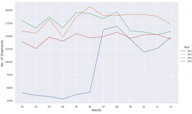
Our sponsor is a large for-hire TL carrier. They provided lane level transactional data for 25 shipper customers across 48 months from January 2016 to December 2019. Each record represents one shipment tendered to the carrier by a shipper on a lane for a given date. The data contains a total of 710,000 transactions across 29,000 distinct lanes where lanes are defined by a Lane ID with corresponding Origin and Destination regions. There could be several unique Lane ID’s within each Origin and Destination Region pair. Exact origin and destination locations were masked for confidentiality. The average length of haul for all the lanes provided in the data set was 477 miles and ranged from 3 miles to 3196 miles. Figure 1 shows the total shipment volume by month across each of the 4 years of data provided.

(22)

Figure 1: A Comparison of Monthly Shipments in 2016 to 2019

The reason we see such a drastically low shipment volume in the first half of 2016 is because the majority of customers’ data started from mid 2016 rather than the start of the year. We included the data from the start of 2016 in our analysis as well.

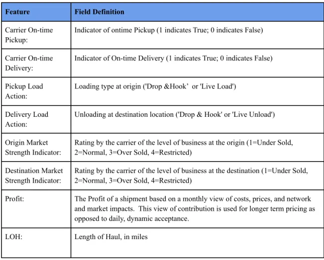
The sponsor also provided us with various shipment characteristics, such as length of haul, shipment margin (profit margin on a given shipment), on-time pick-up and delivery data, pickup and delivery load action (i.e. live, where the driver has to wait, or ‘drop and hook,’ where the shipper preloads a truck to eliminate the waiting and loading time for the driver), origin and destination market strengths (e.g. at a given location, an oversold market means the number of available trucks is less than the demand, and an undersold market means number of available trucks is more than the demand ). Table 2 shows a list of all the features along with their definitions, as used in this study.

(23)

Table 2: Feature Descriptions

Feature Field Definition Carrier On-time

Pickup:

Indicator of ontime Pickup (1 indicates True; 0 indicates False)

Carrier On-time Delivery:

Indicator of On-time Delivery (1 indicates True; 0 indicates False)

Pickup Load Action:

Loading type at origin ('Drop &Hook’ or 'Live Load')

Delivery Load Action:

Unloading at destination location ('Drop & Hook' or 'Live Unload')

Origin Market Strength Indicator:

Rating by the carrier of the level of business at the origin (1=Under Sold, 2=Normal, 3=Over Sold, 4=Restricted)

Destination Market Strength Indicator:

Rating by the carrier of the level of business at the destination (1=Under Sold, 2=Normal, 3=Over Sold, 4=Restricted)

Profit: The Profit of a shipment based on a monthly view of costs, prices, and network and market impacts. This view of contribution is used for longer term pricing as opposed to daily, dynamic acceptance.

LOH: Length of Haul, in miles

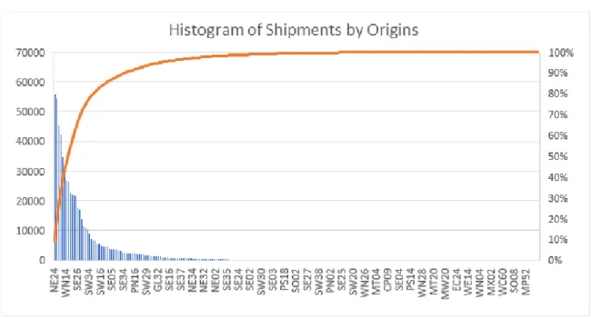
For our analysis, we aggregated individual Lane ID’s by origin regions and analyzed data based on origin level across multiple shippers. The average values of all lanes from an origin region became a feature for that origin. There were two main reasons for consolidating all lane level data by origin region. First, our sponsor manages their network at the origin level, assigning transportation assets by origin. Second, even after we aggregated all the transactions to the origin level across all shippers, many origins still had very low volumes as shown in Figure 2.

(24)

Figure 2: A Histogram of Cumulative Shipments by Origin

The low volume origin regions have very sporadic shipments (see Figure 3). These low volume origins do not have enough volume on a consistent basis in the first place, so looking for churn there does not make sense. We label these origins as ‘Low Volume’ and do not consider them in our churn analysis.

Figure 3: An Example of a Low-Volume Origin

We further segmented the origin regions into high and medium categories because the definition of churn will differ slightly for each. This is discussed in section 3.2.

(25)

Data from 2020 was not included due to the COVID-19 because we wanted to focus on variables pertaining to internal factors that may affect churn (such as shipment and origin characteristics), rather than external variables (such as disruptions due to economic or political reasons or natural disasters). We reasonably assumed that the effects of the pandemic may lead to skewed findings that may not be generalizable to non-COVID times.

3.2 Framework for Identification of Parameters that Define Churn

The three parameters that need to be estimated for a reduction in shipment volume to qualify as churn are as follows:

1. Base: The most appropriate value of baseline volume at a point in time, t, from historical data that can be used as a reference for a churn event. The base volume, Bti, is defined as the previous 26-week rolling average of shipment volume, where t is the time when a potential churn starts and i is the origin.

2. Drop: The minimum amount by which shipment volume needs to decrease for it to be considered the start of churn. This was defined as Dr, and the threshold was set as a 30% reduction in shipment volume from the base volume, Bt, for high volume origins and 100% for medium origins.

3. Duration: The length of time the reduction in volume needs to last for it to be considered as churn. This was set to 13 consecutive weeks.

(26)

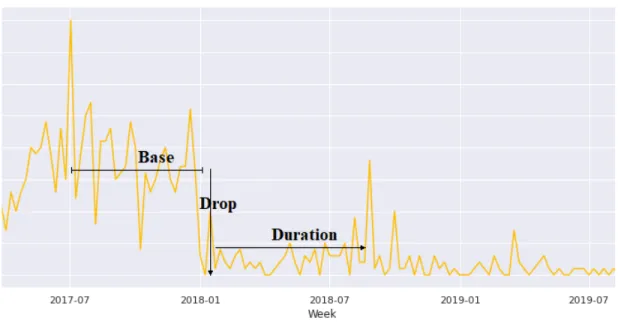
Figure 4: Parameters for defining churn: Base, Drop and Duration

These parameters were calibrated by a combination of practical experience from the sponsor and observation of the data. Each parameter is discussed in turn.

Base - The base volume was initially arbitrarily chosen as a 13-week (equates to a

quarter) rolling average of the shipment volume. The limitation was that this length of period was too short and had a good chance of being affected by quarterly seasonality. We leveraged the experience of the sponsor who expressed that 13-weeks was too short a duration to accurately capture an origin region’s true historical baseline shipment volume. Hence, we changed the duration from 13-weeks to a 26-week rolling average, thereby neutralizing quarterly seasonality to a certain extent, but not capturing any annual seasonality. A year seemed too long to establish a baseline.

Drop - As a starting point, we chose an arbitrary method to determine what

qualified as volume reduction. The first approach that we attempted was a Z score based method. Assuming that shipment volume followed a normal distribution, we defined a

(27)

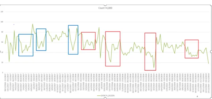
reduction in volume as churn if it was two standard deviations or more away from the base. The standard deviation was the rolling 13-week standard deviation of the shipment volume. One of the limitations of this approach was the assumption that all shipment volume across time always followed a normal distribution. We also noticed that it was very sensitive, only picking the most extreme reductions in volume as illustrated in Figure 5. The blue boxes represent reductions not picked and the red boxes signify reductions that were picked by this method. This selection of the most extreme reductions occurred primarily because our volume reduction threshold (2 standard deviations away from mean) was too strict.

Figure 5: Detected and Undetected Volume Reductions Using Z-score Method

(Blue boxes: reductions not picked, Red boxes: reductions picked by Z method)

To overcome this weakness, we switched to a ‘percentage reduction’ based method where churn occurred if the volume dropped by 50% or more of the historical baseline, Bt. Using this model, it appeared that we were not missing as many drops as the Z score based method. After our discussions with the sponsor we recognized that their priority

(28)

was to ensure that no origins experiencing churn were missed (i.e. avoiding false negatives) and hence the percentage reduction was lowered to 30%, even if this meant an increase in detection of origins that were not churning (false positives). Sensitivity analysis later proved that changes from the 30% threshold did not significantly alter results when compared to a 50% threshold.

As part of our data exploration we also looked at the amount of shipment volumes that each origin region generated across the four years. As described above, we divided origins into 3 categories by shipment volume: high, medium and low. This categorization was important as we made the assumption that churn would look different for an origin region with an average of 300 shipments a week compared to an origin region with only 4 shipments a week. A 30% drop in the former example (loss of 90 shipments/week) would be a very significant drop compared to a 30% drop in the latter (loss of 1 shipments/ week). Similarly, dropping 4 shipments would be trivial in the first case and dramatic in the second. Based on this discussion, we tailored our definition of drop according to the category of origin volume. Low volume origins were not included in our analysis for reasons outlined previously.

Duration - The duration is important to be able to differentiate minor or

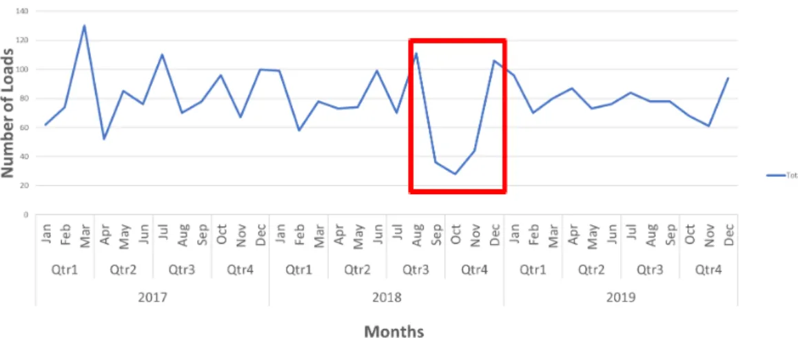
inconsequential volume drops from major ones that could qualify as churn. Previous research in other industries used durations from 6 days to 6 months based on practical characteristics. The TL data had examples of both short drop durations (Figure 6) and permanent, churn-like durations (Figure 7).

(29)

Figure 6: A Temporary Reduction in Volume

Figure 7: A Permanent Reduction in Volume

Based on these observations and advice from our sponsor, we set the required duration of a volume reduction to a minimum of 13 consecutive weeks. The sponsor was willing to accommodate less than one quarter’s worth of persistently low volume in the hope that the volume would eventually be salvaged. If the volume remained low for 13-weeks or more, they would then actively look for a new shipper or reallocate their assets where they could be better utilized.

(30)

To summarize, churn is defined as follows for each type of origin:

1. High volume (Base Volume >5 loads/week at least once during 4 year time

horizon): Churn occurs if volume from an origin drops 30% or more from a base

of 26-week rolling average for a duration of 13 or more consecutive weeks.

2. Medium volume (Base Volume =1-4 loads/week at least once during 4 year

time horizon): Churn occurs if volume from an origin drops by 100% from a base

of 26-week rolling average for a duration of 13 or more consecutive weeks. 3. Low volume (Base Volume <1 load/week for the whole time time horizon):

Churn not assessed because these origins do not have sufficient volume on a consistent basis

3.3 Identification of Churn

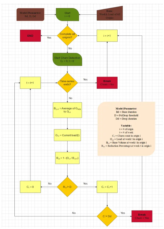
Having defined churn, we then created an algorithm to identify churn based on the definition. For each origin, we started by calculating the base (26-week rolling average of weekly shipment volume) during the first 26 weeks of the 4 years period. Once the base was initialized, we monitored shipment volume week by week until we got to the end of the time horizon of our 4 years of data (Dec 2019). We also updated the value of base as we moved forward each week. If during the period the shipment volume drops, as per our definition, we started the churn counter and froze the base value to the value it was just prior to the time of the drop. Each week that the shipment volume was below our drop threshold, we incremented the churn counter by one. If the degradation of volume remained below the threshold for 13 consecutive weeks, we marked the origin region as under consideration as having a churn event. If the weekly shipment volume rose above the drop threshold before 13-weeks, we recalculated the base and set the counter back to

(31)

zero, and continued monitoring weekly shipment value for a drop. We repeated for all origins.

The pseudo code below is for detecting high volume origins. The algorithm for detecting medium volume origins is exactly the same except that the percentage of volume reduction (depicted below by DropThreshold) is 100% instead of 30% for high volume origins.

---Parameter (Adjustable by users)

BaseDuration - Duration of moving average for ‘Base’

DropThreshold - Reduction ratio that is justified as a significant reduction for ‘Churn’ DropDuration - Duration of significant drops for an origin to be considered as ‘Churn’

Variables

origin_no = origin ID

time = # of week in time series of each ‘origin_no’

ChurnStatus = Churn status of each origin (‘Churn’ or ‘No Churn’) ChurnCount = Count of current consecutive reduction duration (weeks) Base = Moving average of 26 weeks before current time (Base volume)

Reduction = Reduction ratio of the current load from ‘Base’. The ratio is set to 30% for high-volume origins, 100% for medium-volume origins

Data

1. origin_list - a list of Origin ID’s

2. time_series_database - a table of shipment counts by week and origin with the origin ID in one axis and the week numbers in another

---Pseudo Code:

# Parameter Declaration #

BaseDuration = 26

DropThreshold = 0.30 (1.00 for medium-load origins) DropDuration = 13

# Data #

origins = download(origin_list)

(32)

# Start #

origin_no = 0

while origin_no < total_item(origins) do

ChurnCount = 0 ChurnStatus = 0 time = 0

this_time_series = time_series_database[origin_no]

while time < total_time(this_time_series) do

Base = this_time_series[T] / BaseDuration

𝑇 = 𝑡 − 𝐵𝑎𝑠𝑒 𝐷𝑢𝑟𝑎𝑡𝑖𝑜𝑛 𝑡 − 1

∑

Reduction = 1- (this_time_series[time] / Base)

if Reduction > DropThreshold do ChurnCount = ChurnCount+1 if ChurnCount > DropDuration do ChurnStatus = 1 break while end if else do ChurnCount = 0 end if time = time+1 end while origin_no = origin_no+1 end while

(33)

(34)

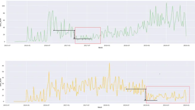
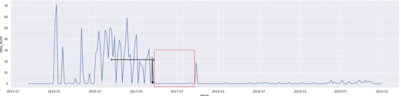
In the first graph shown in Figure 9, at the end of the first quarter of 2017, we see a drop in the base from about 35 loads/week to about 8 loads per week which is >30% reduction, for 30 consecutive weeks, satisfying our definition of churn. It is worth noting that the volume picks up in 2018. This is an example of an origin where the volume eventually came up but it is still labeled as an origin churn because the duration of the drop from the base lasted long enough to have an impact on the carrier’s business. The second graph in Figure 9 illustrates a drop from the base from about 20 loads/week to 3 loads/week for at least a year, meeting criteria for churn as well. The third graph in Figure 9 shows a drop from the base of 20 loads/week to 0 loads/week in mid 2017 for a prolonged period of time and the shipment volume never comes back up. In this example, we are seeing a permanent shift in volume. As long as they meet the three parameters, these origins are also classified as experiencing churn.

(35)

While our identification process for churn differs for high and medium volume origins, once churn is identified at an origin, they are treated the same.

Table 3 summarizes the segmentation of origins by volume and the percentage of origins that experienced churn by segment.

Table 3: Summary of Origins Experiencing Churn by Different Origin Segments

Total Number of Origins Number of Churn Origins % of Churn Origins

High 93 18 19.4%

Medium 57 21 36.8%

Low 105 N/A N/A

(36)

4 - Churn Detection

In this chapter we develop models to detect churn in origins. In our first model we explore whether we can use a certain number of weeks of volume ‘drop’ from the ‘base’ to accurately detect whether our origin would experience actual churn (a consecutive drop of 13 weeks) as per our definition. For example, how likely is it for an origin to experience actual churn (a consecutive 13 weeks of drop in volume from the base) if it had a drop-in volume for, say 4 consecutive weeks?

Next, we explore whether we can improve the accuracy of detection of origin churn by monitoring origin characteristics/features during the detection period. For example, is a higher or lower value of average origin profit margin during the detection period correlated with an origin eventually experiencing actual churn? We leverage decision trees to identify origin characteristics/features and their threshold values that cause churn at an origin region. Finally, we compare a few different lengths (2-week and 3-week) of detection periods to determine which detection period gives us the highest accuracy in detecting eventual churn.

4.1 Importance of Detection

For our sponsor, and other carriers in general, it is important to detect future churn as quickly as possible so that they can act to mitigate the ill effects of churn. For example, if the carrier can detect that a given origin will churn in the future, they can proactively start looking for new customers to compensate for the expected loss of shipment volume at the origin, or reach out to the customer to gain more information. Alternatively, they

(37)

could look for shipment volume from other origins to go to the same destinations as before. To elaborate, suppose a carrier is transporting freight from Miami (origin) to Atlanta (destination A) and Miami to Nashville (destination B). If the carrier believes that the origin in Miami is likely to churn, then they can either find other customers from Miami or find another origin that will go to the same destinations (Atlanta and Nashville) that were linked to Miami. Either way, they can rebalance their network by detecting churn before it occurs in their network.

4.2 Base Model

Per our sponsor’s request, we explored whether, for every origin, we could use the

minimum number of consecutive weeks of ‘drop’ (30% reduction for high volume origins

and 100% reduction for medium volume origins) from the ‘base’ (26-week rolling average of shipment volume) as a signal to detect actual churn (a drop from the base that lasts for a consecutive 13 weeks). For example, we wanted to investigate whether we use a 4-week drop in volume (or any other length of consecutive weeks of volume drop) from the base as an accurate detector of actual churn, i.e., the drop lasted for 13 weeks. In other words, could we determine the probability of actual churn given a certain minimum number of consecutive weeks of drop in volume from the base? The number of minimum weeks we looked at as a signal to detect impending churn was defined as the ‘detection period. Fig 10 shows churn detection accuracy charted against various detection periods in weeks for both high and low volume lanes. Accuracy here is defined as the percentage of origins that had actual churn if churn was detected based solely on a given number of weeks of consecutive drop.

(38)

Figure 10: An Elbow Analysis of Detection Accuracy by Detection Period

In Figure 10, the x-axis represents the length of the detection period in weeks. For example, the value of 2 on the x-axis means a minimum of two weeks of consecutive drop in volume from the base was the detection period. The corresponding value for the two weeks is 25% for high volume origins and 38% for medium volume origins. This means that out of all the high volume origins that had at least 2 weeks of volume drop, 25% went on to experience churn. In other words, based on our data, the detection accuracy of a 2-week detection period is 25% for high volume origins. Note that the detection period should be less than 13 weeks since at 13 consecutive weeks of volume drop, actual churn materializes as per our definition. It is interesting to see that, for origin segments, a 2-week detection period is no more accurate than a 1-week detection period. However, after the 2-week mark, detection accuracy rises very quickly. Comparing the line of high volume origin accuracy to the line of medium volume origin accuracy, we see that for medium volume origins, the increase in accuracy is slower compared to high

(39)

volume origins but it starts at a higher accuracy to begin with. Until week 5, medium volume origins have a higher detection accuracy.

Our sponsor felt that any detection period of 5 weeks or more would not give them enough time to prevent or react to churn. Similarly, they felt that a 1 week detection period was too early to realistically detect churn. Hence, our base model consisted of churn detection using detection periods of 2, 3 and 4-weeks.

4.3 Binary Classification (Decision Tree)

To improve the accuracy of our base detection model, we wanted to learn whether we could use origin characteristics/features in addition to the length of the detection period. Essentially, we wanted to know whether, if we monitored origin characteristics before and after the drop for the length of the detection period, we would be able to more accurately detect churn in an origin. For example, if the detection period was 3 weeks, we wanted to see whether the average origin profitability (or any combination of characteristics/features) during 3 weeks before or after the drop, could be used to classify whether an origin would churn or not. In other words, we needed to fit a binary classification model to classify churn from a ‘temporary’ drop in volume from origin characteristics during a detection period. In total, we will develop 6 models. 2-, 3- and 4-week detection models for high volume origins and 2-, 3- and 4-week models for medium volume origins. Origin characteristics that are observed before the drop are labelled ‘Pre-Drop’ and origin characteristics observed after the drop are labelled ‘Post-Drop’.

To prepare our data for our binary classification model, we first extracted all the origins that had at least a 2-week drop from the base. For the origins that met the criteria

(40)

of churn (13 weeks of consecutive drop from the base), each was labelled ‘Churn Origin’. For the origins that had at least 2 weeks of drop from the base but less than 13 weeks of drop from the base, each was labeled ‘Transient Drop Origin’. We took 2-week averages of all the origin characteristics/features before the drop and after the drop and repeated the same process for the 3-week and 4-week detection periods to get three datasets, one for each detection period. In our final fully prepared datasets that would be inputted to a classification model, each row represented an origin and had a unique origin identifier, the value of the target variable (1 if origin was labelled ‘Churn Origin’ and 0 if ‘Transient Drop Origin’) and detection period averages of the origin characteristics .

We ran a decision tree on our input data to classify origins as ‘Churn Origin’ or ‘Transient Drop Origin’ based on the values of our features (detection period averages of origin characteristics). For each origin segment (high or medium) a decision tree classification model was developed for each of the three detection periods. We used the Orange software, which is an open-source data visualization, machine learning and a data mining toolkit. It features a visual programming front-end for explorative rapid qualitative data analysis and interactive data visualization.

Before analyzing the results of each detection period decision tree, it is important to clarify a few points that are common to all three detection period decision tree models. First, we separated 20% of the data from each of the three different detection period input datasets. This way we could test each resulting model with new or ‘unseen’ data. Second, to compare the detection/prediction power of each model, we employed k-folds cross validation to train our data. k was set to the total number of observations in the dataset such that each observation (an origin with its actual label, classification and detection

(41)

period characteristics) was given a chance to be held out of the dataset. Essentially, we held out one instance at a time, inducing the model from all others and then classifying the held out instances. This method allowed us to compare our models using all the observations available. A useful aspect of this cross validation method is that each decision tree created for each fold is very similar since they only differ by one observation.

The goal of k-fold cross validation is to determine which detection period is the most accurate in detecting origin churn. To evaluate the detection of each decision tree after k-fold cross validation, we used a confusion matrix. The confusion matrix is a simple way to illustrate how many times we classified correctly and how many times we classified incorrectly for each value of the target variable (‘Churn Origin’ vs ‘Transient Drop Origin’). Each row in a confusion matrix represents the instances in an actual class (in our case ‘Churn Origin’ or ‘Transient Drop Origin’), while each column represents the instances in a predicted class. Since we have two target variables, we have a 2x2 matrix, shown in Table 4.

Table 4: A Confusion Matrix Template

Predicted 'Churn Origin' Predicted 'Transient Drop' Actual 'Churn Origin' True Positives (TP) False Negatives (FN)

Actual 'Transient Drop' Origin False Positives (FP) True Negatives (TN)

Each column in a confusion matrix captures a specific outcome:

(42)

False Negatives (FN) is where origins twere classified as Transient Drop Origins, but actually had churn.

False Positives (FP) is where origins were classified Churn Origins, but in fact did not experience churn.

True Negatives (TN) is where origins were classified correctly as Transient Drop Origins.

There are many ways to measure how well a classification model is working. We used the following performance metrics of the confusion matrix to evaluate the performance of models:

● Sensitivity: The proportion of Churn Origins that were correctly predicted as Churn Origin. (Sensitivity = _{𝑇𝑃 + 𝐹𝑁}𝑇𝑃 )

● Accuracy: The proportion of All Origins that were correctly predicted. (Accuracy = _{𝑇𝑃 + 𝑇𝑁 + 𝐹𝑃 + 𝐹𝑁}𝑇𝑃 + 𝑇𝑁 )

● MCC: Another quality measure for a classification model. 1 means all predicted data are correct. -1 means all predicted data are incorrect. 0 means predicted data are random and the classification model cannot distinguish data at all (MCC =

) 𝑇𝑃 𝑥 𝑇𝑁 − 𝐹𝑃 𝑥 𝐹𝑁

(𝑇𝑃 + 𝐹𝑃)(𝑇𝑃+𝐹𝑁)(𝑇𝑁+𝐹𝑃)(𝑇𝑁+𝐹𝑁)

While we consider all of the performance metrics above, the most important one for us is sensitivity. This is because our sponsor would rather have a low false negative rate then a high false positive rate. It is preferable to predict churn when there is none

(43)

compared to not predict churn when there is churn. In other words, a false alarm is significantly less costly than a missed fire.

4.4 Decision Tree Comparison ForHigh Volume Origins

For each Origin Type and each detection period input dataset, we trained our decision tree using the 80% of the dataset to get the following decision tree results.

4-week detection period:

The characteristic for each split in the tree is at the bottom of the box. The value for each split is listed at each leg. For example, the first split occurs if the average drop is greater than or less than 79.4%. Of the 46 high volume origins that have at-least 4 weeks of drop, 32 fall below and 14 fall above. For the 14 origins above this threshold, 12, or 85.7%, experienced churn. The heading of each bucket in bold indicates the prediction of the decision tree, for example in the bucket labelled three, the prediction of the decision tree

(44)

was ‘Transient Drop Origin’ and 8 out of the 10 origins that fell under that bucket experienced only a transient drop in volume.

The tree above has four terminal buckets labelled 1, 2, 3 and 4. Every Origin will lie in one of these four buckets:

1. If the average 4 week [drop is less than 80% and the average origin market

strength post drop is less than 2.35 (normal market) then the probability of churn is 0% and our binary classifier will classify the origin as not having future churn (Transient Drop Churn).

2. If the average 4 week drop is less than 80%, and the average destination market strength post drop is greater than 2.35 but less than or equal to 4.25, then there is a 40% probability of churn and our binary classifier will classify the origin as not having future churn.

3. If the average 4 week drop is less than 80%, and the average destination market strength post drop is greater than 2.35 and greater than 4.25, then there is a 20% probability of churn and our binary classifier will classify the origin as not having future churn.

4. If the average 4-week drop is greater than 80%, then there is a 85.7% probability of churn and our binary classifier will classify the origin as having future churn.

(45)

1. If the average 3-week drop is less than or equal to 78%, and the average origin market strength post drop is less than or equal to 1.7 (under sold market) and average profitability of a shipment from that origin is less than or equal to 321, then there is a 46.2% probability of churn and our binary classifier will classify the origin as not having future churn.

2. If the average 3-week drop is less than or equal to 78%, and the average origin market strength post drop is less than or equal to 1.7 and average profitability of a shipment from that origin is greater than 321, then there is a 0% probability of churn and our binary classifier will classify the origin as not having future churn. 3. If the average 3-week drop is less than or equal to 78%, and the average origin

market strength post drop is greater than to 1.7, then there is a 0% probability of churn and our binary classifier will classify the origin as not having future churn.

(46)

4. If the average 3-week drop is greater than 78%, then there is a 70.6% probability of churn and our binary classifier will classify the origin as having future churn.

The tree above has five terminal buckets labelled 1, 2, 3, 4 and 5. Every Origin will lie in one of these five buckets:

1. If the average 2-week drop is less than or equal to 64%, and % of drop and hook pick ups post drop is less than or equal to 1.5, then there is a 15% probability of churn and our binary classifier will classify the origin as not having future churn. 2. If the average 2-week drop is less than or equal to 64%, and the % drop and hook

pick up post drop is greater than 1.5, then there is a 0% probability of churn and our binary classifier will classify the origin as not having future churn.

3. If the average 2-week Drop is greater than 64%, and the number of total loads out of an origin is less than or equal to 2273, and the drop is less than or equal to 82%, then there is a 36% probability of churn and our binary classifier will classify the origin as not having future churn.

(47)

4. If the average 2-week drop is greater than 64%, and the number of total loads out of an origin is less than or equal to 2273, and the drop is greater than 82%, then there is a 82% probability of churn and our binary classifier will classify the origin as having future churn.

5. If the average 2-week drop is greater than 64%, and the number of total loads out of an origin are greater than 2273, then there is a 23% probability of churn and our binary classifier will classify the origin as not having future churn.

Table 5 shows the threshold values of origin characteristics by detection period for high volume origins.

Table 5: Origin Characteristic Threshold Values by Detection Period For High Volume

Origins

Characteristic/Feature 2-week 3-week 4-week

Base N/A N/A N/A

Drop 81% N/A N/A

AverageDropDuringDetectionPeriod 63% 78% 80%

% On Time Pick Up (Pre Drop) N/A N/A N/A

% On Time Delivery (Pre Drop) N/A N/A N/A

% Drop and Hook Pick Up (Pre Drop) N/A N/A N/A

% Drop and Hook Delivery (Pre Drop) N/A N/A N/A

Average Origin Market Strength (Pre Drop) N/A N/A N/A Average Destination Market Strength (Pre Drop) N/A N/A N/A

Average Length of haul (Pre Drop) N/A N/A N/A

Average Origin Profit (Pre Drop) N/A 321 N/A

% On Time Pick Up (Post Drop) N/A N/A N/A

% On Time Delivery (Post Drop) N/A N/A N/A

% Drop and Hook Pick Up ((Post Drop) 1.50% N/A N/A

% Drop and Hook Delivery (Post Drop) N/A N/A N/A

Average Origin Market Strength (Post Drop) N/A 1.711 2.35 Average Destination Market Strength (Post Drop) N/A N/A 3.25

Average Length of haul (Post Drop) N/A N/A N/A

(48)

The average drop during the detection period is the most important characteristic in detecting churn. It is the first characteristic that all three detection models use to split data for classification. 3-week and 4-week detection models both further use Average Origin Market Strength to classify origins but differ in the final characteristic they use. The 4-week model uses Average Destination Market Strength while the 3-week model uses Average Origin Profit (Post Drop). The 2-week detection model differed significantly from the 3-week and 4-week models after the first split. It used % of Drop and Hook (Post Drop), Total loads and Drop to classify data.

4.5 Confusion Matrix Comparison on Training Data For High Volume Origins

After running a decision tree-based k-folds cross validation on 80% of the dataset created for each detection period (2-week, 3-week and 4-week), we get the following Confusion Matrices.

(49)

3-week detection period

In each confusion matrix we see the sum of the first row of the confusion matrix gives us the total origins with churn in the dataset for the detection period. The top left quadrant in the first row gives the number of instances our detection model correctly classified origin churn. The sensitivity of each confusion matrix is the number of correctly identified churn origins (top left quadrant) divided by the number of actual origin churns (sum of the first row).

Table 6 shows a comparison of performance metrics of each of the three detection models on training data.

(50)

Table 6: Training Set Performance Metrics for High Volume Origins

Training Performance Metrics Sensitivity Accuracy MCC

4-week 66% 71% 0.40

3-week 66% 77% 0.46

2-week 50% 68% 0.22

The reason the total number of observations is greater as we move from a 4-week to 3-week detection model is because the number of origins with at least 4 weeks of churn is a subset of the number of origins with at least 3 weeks of churn.

4.6 Confusion Matrix Comparison on Test Data For High Volume Origins

Finally, we tested our three decision trees trained on 80% of their respective datasets on our 20% test data that was set aside at start. This was done to compare how the detection models perform on unseen data, as would be the case when the sponsor uses our model to detect churn in the future.

(51)

Table 7 shows a comparison of performance of metrics of each of the three detection models on test data:

Table 7: Testing Set Performance Metrics for High Volume Origins

4-week 100% 92% 0.82

3-week 100% 93% 0.83

2-week 0% 65% -0.21

4.7 Results For High Volume Origins

Our Confusion Matrix comparison on the training set as well as on the test set show that a 3-week detection model outperforms both 2-week and 4-week detection models for High Volume Lanes. Even though 3-week and 4-week detection have the same Sensitivity

(52)

in the training and test data, a 3-week is always preferred since it gives carriers more time to respond to churn. Our 3-week detection model gave us a 66% of accurately detecting churn (sensitivity) on the training set and a 100% chance of accurately detecting churn on the testing set. This is a big improvement from a 38% accuracy of detecting churn in the base model.

Our results seem to suggest that our training models were not overfit which is why they performed so well on the testing set. Looking at the MCC, we see the same result that the 3-week and 4-week models have moderate detection power in the training set and a high detection power in the test set. However, since the data was sparse, we were cautious in its interpretation.The exceptionally small set of origins used can inaccurately skew results in one direction and can lessen the value of the predictions.

In Figure 11, we have shown how 3-week and 4-week decision tree-based detection models lead to an increase in accuracy of detecting churn origins, when compared to 3-week and 4-week base detection models. Looking at Figure 11, we see that when there is a minimum of 3 weeks of drop, the accuracy of detecting churn origins (sensitivity) is 28%. However, if we monitor origin characteristics during the 3-week drop, we can improve the accuracy of detecting origin churns considerably. Our results from a 3-week decision tree based detection model improved the accuracy from 28% to 66%, on training data. This is represented by the red line. Similarly, the same 3-week decision tree based model improved the accuracy of detecting origin churns from 28% to 100%, on testing data. This is represented by the green line.

(53)

Figure 11: An Elbow Analysis of Detection Accuracy with The Decision Tree

4.8 Decision Tree Comparison For Medium Volume Origins

For medium volume origins, it is important to note that we do not have any data for post drop characteristics. This is because we have defined the drop in medium volume origins as a 100% reduction which does not leave any shipments/transactions and in turn characteristics to monitor post drop.

(54)

1. The tree above has three terminal buckets labelled 1, 2 and 3. Every Origin will lie in one of these three buckets:

2. If the base volume is less than or equal to 0.62 shipments/week, then there is an 82% probability of churn and our binary classifier will classify the origin as having future churn.

3. If the base volume is greater than 0.62 shipments/week, and the average origin market strength is less than or equal to 2, then there is a 20% probability of churn and our binary classifier will classify the origin as not having future churn.

4. If the base volume is greater than 0.62 shipments/week, then there is a 30% probability of churn and our binary classifier will classify the origin as not having future churn.

(55)

1. If the pre-drop average profitability of a shipment from an origin is less than or equal to -18, then there is a 10% probability of churn and our binary classifier will classify the origin as not having future churn.

2. If the pre-drop average profitability of a shipment from an origin is greater than -18, and the base volume is less than or equal to 1.46 loads/week, and the average profitability of a shipment is greater than 107, then there is a 60% probability of churn and our binary classifier will classify the origin as having future churn. 3. If the pre-drop average profitability of a shipment from an origin is greater than

-18, and the base volume is less than or equal to 1.46 loads/week, and the average profitability of a shipment is less than or equal to 107, then there is a 90% probability of churn and our binary classifier will classify the origin as having future churn.

4. If the pre-drop average profitability of a shipment from an origin is greater than -18, and the base volume is greater than 1.46 loads/week, then there is a 25% probability of churn and our binary classifier will classify the origin as not having future churn.

(56)

2-week detection

The tree above has three terminal buckets labelled 1, 2 and 3. Every origin will lie in one of these three buckets:

1. If the base volume is less than or equal to 0.62 shipments/week, then there is an 82% probability of churn and our binary classifier will classify the origin as having future churn.

2. If the base volume is greater than 0.62 shipments/week, and the average profitability of a shipment from an origin is less than or equal to 241, then there is a 12% probability of churn and our binary classifier will classify the origin as not having future churn.

3. If the base volume is greater than 0.62 shipments/week, and the average profitability of a shipment from an origin is greater than 241, then there is a 30% probability of churn and our binary classifier will classify the origin as not having future churn.

(57)

Table 8 shows the threshold values of origin characteristics by detection period for medium volume origins.

Table 8: Origin Characteristic Threshold Values by Detection Period For Medium

Volume Origins

Characteristic/Feature 2-week 3-week 4-week

Base 0.62 1.46 0.62

Drop N/A N/A N/A

AverageDropDuringDetectionPeriod N/A N/A N/A

% On Time Pick Up (Pre Drop) N/A N/A N/A

% On Time Delivery (Pre Drop) N/A N/A N/A

% Drop and Hook Pick Up (Pre Drop) N/A N/A N/A

% Drop and Hook Delivery (Pre Drop) N/A N/A N/A

Average Origin Market Strength (Pre Drop) N/A N/A N/A Average Destination Market Strength (Pre Drop) N/A N/A N/A

Average Length of haul (Pre Drop) N/A N/A N/A

Average Origin Profit (Pre Drop) 241 -18 and 117 N/A

% On Time Pick Up (Post Drop) N/A N/A N/A

% On Time Delivery (Post Drop) N/A N/A N/A

% Drop and Hook Pick Up ((Post Drop) N/A N/A N/A

% Drop and Hook Delivery (Post Drop) N/A N/A N/A

Average Origin Market Strength (Post Drop) N/A N/A 2 Average Destination Market Strength (Post Drop) N/A N/A N/A

Average Length of haul (Post Drop) N/A N/A N/A

Average Origin Profit (Post Drop) N/A N/A N/A

The base is the most important characteristic in detecting churn for Medium Volume Origins. It is the first characteristic that all three detection models use to split data for classification. 2-week and 3-week models use the same second characteristic of Average Profit (Pre-drop) but significantly different thresholds. The 4-week model uses Average Origin Market Strength (Post Drop) as its second characteristic. It is also interesting to note that medium volume only use 2 characteristics for classification

(58)

compared to three from the high volume models. Moreover, these characteristics for medium volume models are mostly different from those for high volume models.

4.9 Confusion Matrix Comparison on Training Data for Medium Volume Origins 4-week detection

(59)

Table 9: Training Set Performance Metrics for Medium Volume Origins

4-week 68.4% 76% 0.52

3-week 68.4% 77% 0.54

2-week 68.4% 79% 0.57

4.10 Confusion Matrix Comparison on Test Data for Medium Volume Origins