The design and implementation of a laser range-finder array for robotics applications

The Design and Implementation of a Laser

Range-Finder Array for Robotics Applications

by

Will Vega-Brown

Submitted to the Department of Mechanical Engineering

in partial fulfillment of the requirements for the degree of ssTsINSiTlrL

OF TECH-NIOLOGY

Bachelor of Science in Mechanical Engineering

I

OCT

2 0

2011

at the

LSr-IBRRIES

MASSACHUSETTS INSTITUTE OF TECHNOLOGY

ARCHIVES

June

2011

@

Will Vega-Brown, MMXI. All rights reserved.

The author hereby grants to MIT permission to reproduce and

distribute publicly paper and electronic copies of this thesis document

in whole or in part.

Author...

Department of Mechanical Engineering

May12, 2011

Certified by... ... ... ...

Sangbae Kim

Assistant Professor

Thesis Supervisor

Accepted by...

..

...

John Lienhard

Undergraduate Officer

The Design and Implementation of a Laser Range-Finder

Array for Robotics Applications

by

Will Vega-Brown

Submitted to the Department of Mechanical Engineering on May 12, 2011, in partial fulfillment of the

requirements for the degree of

Bachelor of Science in Mechanical Engineering

Abstract

We introduce the concept of using a laser range finder array to measure height and tilt for mobile robotics applications. We then present a robust, scalable algorithm for extracting height and tilt measurements from the range finder data. We calibrate the sensors using a precision two-axis system, and evaluate the capabilities of the sensors. Finally, we utilize the sensors and the two-axis system for imaging to illustrate their accuracy.

Thesis Supervisor: Sangbae Kim Title: Assistant Professor

Acknowledgments

The author would like to thank Professor Sangbae Kim for his help and guidance, as well as Albert Wang for his assistance throughout the thesis process.

Contents

1 Introduction 11

2 Theoretical Analysis of Sensor Array Data 13

2.1 Transforming measurements . . . . 13

2.2 Error Mitigation... . . . . . . . . 18

3 Calibration and Evaluation of Sensors 21

3.1 Design of Testing Unit . . . . 21

3.2 C alibration . . . . 23

3.3 Im aging . . . . 27

List of Figures

3-1 First design iteration . . . . 22

3-2 Second design iteration . . . .. . . . 23

3-3 Labview code used to control scans . . . . 24

3-4 Laser sensor ranging a plane . . . . 25

3-5 Range versus measured current . . . . 26

3-6 Depth mapping of an area of the lab. Color denotes distance from cam era. . . . . 27

1

Introduction

In many underactuated robotic systems there is a need for independent measurement of the orientation of some part of the robot relative to the ground - independent, that is, in the sense that the data should come directly from sensors and not from reverse kinematics. Generating data from the configuration of the limbs of a robot becomes futile when those limbs are off the ground. An extreme case is a running robot, which may at some point have all legs off the ground at once. In order to generate new control signals, the robot must have access to reliable sensor data, regardless of the configuration and position of the robot. One such sensor system is an array of laser range-finders, and it is this array system which forms the focus of this paper.

The principle of operation is simple; a set of sensors are arranged such that they all face the ground at slightly different angles. The distance from each sensor to the flat ground is then measured, and relevant information, like height and tilt, is extracted using trigonometric and linear algebraic techniques. In this paper, we resolve two barriers to the construction of such a system. First, we explore the methodology of extracting the desired information from sensor data, and present a robust and scalable algorithm for performing this extraction. Second, we calibrate and evaluate one of the laser sensors; this calibration is an essential step towards getting reliable data out of an array. Finally, to demonstrate the calibration, we use the laser sensor for imaging, illustrating its accuracy and ranging abilities.

2

Theoretical Analysis of Sensor

Array Data

The ultimate goal of this research is the creation of a sensor array composed of multiple laser rangefinders. If each rangefinder is pointed downwards in a slightly different direction, then so long as the ground is reasonably flat, the array data can be processed to obtain useful information on the location of the array relative to the ground. Specifically, it will be able to discern the distance normal to the ground

- the height of the array - as well as its angle relative to the ground, in the form

of pitch and roll angles or in some other equivalent form. By utilizing a variety of techniques, the rangefinder array can quickly, accurately and robustly generate this data, for integration into the control loops of mobile robots.

2.1

Transforming measurements

In the most general case, we may have an arbitrary number of sensors n, each with a location and orientation fixed relative to some reference frame attached to the moving platform. The ith sensor, then, may be parameterized by its position pi, its heading v,

and the range it reports, xi. Our goal, then, is to find the orientation and position of the moving reference frame relative to the surface the lasers see. Solving this problem directly via trigonometry is a difficult and messy process which leads to unwieldy

solutions for n > 4; however, by recasting the problem in the language of linear algebra, we can avoid unnecessary trigonometry and make the problem tractable.

First, note that the inverse problem is comparatively easy; given a known position and orientation, finding the expected range reported by a sensor is simply a matter of applying the appropriate sequence of transformations. Taking a single range mea-surement closes a vector loop which begins and ends in the plane we are measuring against. That is, it creates a chain of vectors connected head-to-tail, which begin and end in a known plane. Letting P be the position of the mobile frame origin in the lab frame, and R be the rotation which takes vectors from the lab frame into the mobile frame, the chain can be expressed as

V = P + Rpi + Rxii

This vector must be confined to the plane we measure against. Thus, if we choose our lab frame such that 2 is orthogonal to that plane, we have

v z= (P + Rpi + Rxihi) - i= 0

This reduces to

Rz(pi + xihi) = 0 (2.1)

where R =

(

cos(O) sin(#) cos(O) cos(#) sin(9) P2

)

is a row vector

correspond-ing to the z-component of the rotation and translation. Here, Pz is the height of the mobile frame above the plane, and we have chosen 6 to be roll and

#

to be pitch. Note pi and hi are four-vectors:

Pi1

0

If we knew the position and orientation of the mobile frame - that is, if we knew

0,

#,

_{z, obtaining x would simply be a matter of solving equation 2.1. Given n sensors,}

then, we have a set of n equations relating the orientation of the mobile frame to the n measurements xi. This can be represented as a single matrix equation:

Plx P2x ... Pnx h₁x h₂x -- hn x 0 ... 0

RT Piy P2y Pny hiy h2y - hn 0 X2 -- 0

Plz P2z ... Pnz h1z h2z -- hnz - 0

1 1.-- 1 0 0 --- 0 0 0 --- xn

(2.2) To simplify the rest of the problem, we define a matrix X as

T Plx P2x ... Pnx h₁ h₂x --x nx 0 ... 0

Ply P2y - Pny + hiy h2y hny 0 X2 -.- 0

Plz P2z - Pnz h₁ h2z - - : --. 0

1 1.- 1 0 0 ... 0 0 0 ... xn

(2.3)

Taking the transpose of equation 2.2 we have a reduced matrix equation,

XRZ = 0 (2.4)

Our goal is to obtain the matrix Rz, in which is encoded our orientation infor-mation, from a measured matrix X. Note first that the tractability of the problem is dependent on n. As might be expected, for n < 3, the system is underdefined, and there are an infinite number of solutions; in this case, there is insufficient information to determine the orientation of the mobile frame. Additionally, for n > 3, the system is overdefined; since our measurements are subject to noise, our matrix X will be imperfect and the system will frequently be impossible to solve exactly. Only for n = 3 are we strictly guaranteed a solution; we will begin our analysis there.

In this n = 3 case, the problem is reduced to finding the nullspace of the matrix X. While there are many methods of doing this, the one which is indicative here is

to first diagonalize the system, then recognize that the eigenvector corresponding to a zero eigenvalue lies in the nullspace of X. To do this, we first square the system by multiplying by XT, then choose an appropriate method for diagonalization.

Most of these problems are mitigated by using a larger number of sensors. In the presence of error, the system will become unsolvable; however, we can employ projective methods to obtain a nearest solution, in the least-squares sense. We begin

by squaring the system and defining a quantity e:

E = XT XR2 (2.5)

We then diagonalize XTX:

XTX = VAV-1 (2.6)

Note that since XTX is symmetric, we can express the eigenvectors in an or-thonormal form, and thus V = VT.

The best solution to equation 2.4 is then the matrix R, which minimizes

l

|2,

the magnitude of e:

lE|2

= RTVA2_{VT R2 (2.7)}

By inspection, this will be minimized by choosing Rz as the eigenvector

corre-sponding to the smallest eigenvalue of the matrix XTX. The fact that the matrix XTX will in general be nonsingular permits us to use a modification of the power method to compute this minimal eigenvector. The power method utilizes the fact that successively multiplying a vector by a matrix will asymptotically map the vector to the eigenvector of that matrix corresponding to its largest eigenvalue:

A nx = dA"vi (2.8)

i=1

Here, Ai denotes an eigenvalue and vi an eigenvector. As n - oc, the largest

the matrix A is nonsingular, however, we may perform the same process the inverse of A; the eigenvalues of the inverse of a matrix are the inverses of the eigenvalues of the original matrix, and as such the largest eigenvalue of the inverse matrix will correspond to the smallest of the original matrix. Thus, to find our eigenvector Rz above, we simply choose an arbitrary vector x, and perform the multiplication as many times as necessary to achieve our desired accuracy:

Rz, = (XTX)- )x (2.9)

The minimal value of n will depend on the typical magnitude of C, and thus will be a function of the accuracy of the sensors. In practice, however, n is typically small, on the order of 2 to 5. One key advantage of this method is that it does not require access to complex numerical libraries; it can be easily coded in any programming language, making it suitable to be run on a microcontroller of the type one might use to drive the sensor system in a mobile robotics application.

We are left with a single degree of freedom in the solution RT: the length of the calculated eigenvector. To obtain the desired result, we impose a normalization on the first three coordinate values of R[.

To do this, we first divide R into two parts such that R = vT

):

v0

=

(

cos(O) sin(#) cos(O) cos(#) sin(O)

)

(2.10)

vi = P (2.11)

Trigonometric identities impose

v Tvo = 1 (2.12)

From this constraint, we can fully deduce the magnitude of RT. If we additionally require Pz to be positive, we restrict the sign of R T; thus, the eigenvector has been completely constrained and the the desired parameters

{0,

#,

z} can be deduced.

The full algorithm can then be defined as below:

1. Collect data from n sensors.

2. Using a previously calculated set of position and heading vectors, calculate the matrix X as in equation 2.3.

3. Compute (XTX) and (XTX)-1 .

4. Choose an arbitrary vector x E R4_{. Compute R2 as in equation 2.9}

5. Normalize R2 as in equation 2.12

6. Extract

{#S,

0, z} from R2 via trigonometry.

This method is scalable to an arbitrary number of sensors, requires no numerically cumbersome calculations, imposes minimal calculation error, and results in output that is nearly optimal, in the sense that it provides the best estimate of the desired parameters, given a set of data.

2.2

Error Mitigation

The use of a linear algebraic framework opens up a realm of possibilities for interesting ways of mitigating errors in the sensor array, as well as accelerating computation. For instance, by computing the change in coordinates rather than the coordinates directly, we can rapidly develop an estimate of the current state. If we define a matrix of measurements A = XTX, with X defined as in equation 2.3, then we may solve the problem once explicitly as in section 2.1, then iteratively for later times. Let the subscript i denote a fully solved initial state AiRi = ERj, and let the subscript

f

denote a later state for which only the measurement matrix Af is known. Thus we have

AiR = esRi (2.13)

We denote variations by A:

Ef = Ei + AC (2.15)

Af Ai + AA (2.16)

Rf Ri + AR (2.17)

If we assume the variations to be small - that is, we assume the update is being

applied after a small time step, or in a slowly varying system - we can neglect second-order terms. Moreover, we assume the variation in e to be negligible; c is a small random variable we expect to vary more or less continuously, and variations in small continuous variables are second order terms. Eliminating the

f

indexed terms in favor of A terms and expanding, we find

AIR + AAR + Ai AR = eRi + Ej AR (2.18)

This can be solved for AR by substitution with equation 2.13:

AR = (eI - Aj)-1 AAR (2.19)

The result provides an accurate estimate of the final coordinate solution R given the new measurements. This solution can be computed significantly faster than can the eigensolution, and using it as an initial guess could potentially reduce the number of iterations required by the initial algorithm. This speed has an additional advantage. Assume one of the laser beams encounters an obstruction. The resulting data will result in output parameters that dramatically deviate from true values, with no way of knowing a priori which beam is giving incorrect data. The only sign of an error will be the large value e generated in the algorithm. However, if the computation can be done quickly enough, an exhaustive search becomes feasible; the algorithm cycles through every combination of beams, starting with all n beams, then all n combinations of n - 1 beams, and proceeding until E drops below a certain threshold.

2. Take the product RTAfRf = 6RTRf. If c is small - with small defined by experiment - then Rf is likely very close to the true eigenvector. If C is large, it is likely an obstruction has occurred.

3. If c is large, repeat the first step n times, where n is the number of sensors;

each time, remove a single sensor from the data. When the result gives a small

E, then the obstructed beam has likely been located.

4. Once the beams generating invalid data are obtained, the full algorithm detailed in section 2.1 may be employed.

Obviously, this will only work if three sensors are providing unobstructed data. This suggests a second benefit to including redundant sensors; in addition to reducing the error constant E, they will provide additional redundancy in the case of an uneven floor or the presence of obstacles.

3

Calibration and Evaluation of

Sensors

The second phase of our project involved the design and fabrication of a two-axis unit to be used to calibrate and evaluate the laser sensors. Once constructed, the unit was used to measure the variation in sensor output current as the beam was scanned over a wall, allowing us to calibrate the unit for a variety of ranges and angles of incidence. The obtained calibration curve was then used to generate a depth-mapped image of the lab; the image provided fair resolution, and some feature extraction was possible.

3.1

Design of Testing Unit

For the purposes of calibrating and evaluating the laser sensors, we create a two-axis rotating platform, driven by precision servos and laser cut for accurate geometry.

The unit was constructed out of laser-cut acrylic. The first design iteration was meant to be assembled, then clamped and glued together with an adhesive (Figure

3-1). This methodology proved unworkable, however; the need for disassembly to

remove the motors and laser sensors made permanent adhesion impractical. Moreover, design flaws in this early iteration became apparent. There was insufficient mechanical support for the pitch axis, which was largely supported by a cantilever action on the motor gear; this resulted in sagging, and made accurate measurement of the position

of the laser sensor difficult.

Figure 3-1: First design iteration

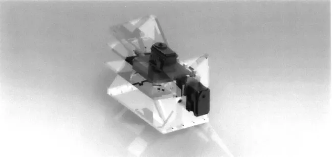
A second iteration was built (Figure 3-2). This iteration supported the pitch axis

with a bearing, and reinforced the yaw assembly with additional material. Rather than glue, this variant employed laser-cut acrylic struts, meant to mate with holes cut in the main body. This design offered two distinct advantages; first, the snap-fit action of the struts held the structure together without the benesnap-fit of adhesives, facilitating assembly and potential disassembly, and second, the struts offered the structure increased rigidity by reinforcing each corner.

The strut-supported assembly did prove troublesome to assemble; because of in-consistencies in the laser kerf, it was difficult to cut mating holes for the struts that interfered enough to provide a good grip, yet not so much as to prohibit assembly. Ideally, multiple sample cuts would have been made and the best size chosen experi-mentally; in practice, we simply made an initial estimate and found it to be less than ideal, yet satisfactory. Although several cracks formed in the acrylic during assembly, none proved structurally fatal.

To drive the unit, we chose two Dynamixel EX-106+ servos. These were chosen primarily because of their high angular positioning resolution; manufacturer specifi-cations claim a angular precision of 0.06', and preliminary evaluation suggested that

Figure 3-2: Second design iteration

precision could be attained quickly and repeatably, both essential in a precision mea-surement unit. The servos had additional advantages, as well; they interface nicely with Labview, they can be daisy chained to simplify wiring and control architecture, and they offer high-torque for their size, guaranteeing enough power to move the sensor assembly quickly.

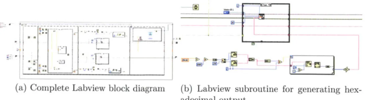
The software implementation was done entirely in National Instruments Labview; the motor drivers, laser data collectors, and high-level control were each written separately, then merged into one larger program (Figure 3-3a). The only complication of note came in the implementation of the motor drivers; the motor accepts commands in hex-code literals, that is, actual four-bit sequences corresponding to the various codes. Outputting such codes is a nontrivial task in Labview, which by default outputs hex code in ASCII characters; the resolution of this issue required a relatively complex subroutine (Figure 3-3b).

3.2

Calibration

To evaluate the accuracy and precision of the Micro-Epsilon range finders, we em-ployed the pan-tilt unit described above. The unit was fixed at a known distance from

(a) Complete Labview block diagram (b) Labview subroutine for generating

hex-adecimal output

Figure 3-3: Labview code used to control scans

a flat plane, and measurements were taken at one degree intervals over a wide variety of angles. The resulting data was fitted to a known form using Matlab's optimization tools.

This form was inferred from predictions relating to the geometry of the unit and three measured parameters: the yaw angle 0, the pitch angle

#,

and the range finder measurement i, measured in mA. The geometry of the unit was obtained from the solid model and verified with direct measurement; the position of the laser point in Cartesian coordinate space can then be obtained via a series of rotations and translations of axes.

We first suppose a linear relationship between the measured current i and the experimental range r; that is, r =c1i + c2. If 61 is a vector between the center of

yaw rotation and the location of the laser emitter, and h is the heading vector of the laser in the rotating yaw frame, then the location of the laser point in the yaw frame is given by 'yaw =J

+

rh. Rotating the frame by the yaw angle 0 and translating by another vector 2 gives the laser point location in the rotating pitch frame; a similar

procedure gives the laser point location in the lab frame. The complete transformation is then given by

r= V3 + R,(#) (V2 + RY()(i ₁ + rh))

By measuring i for a series of angles 0,

#,

we can obtain the parameters ci, c₂ which

interpret the measurements taken by the sensors in other contexts. For instance, the same calibration can be applied to the multi-sensor array, or for use in imaging with the pan-tilt unit.

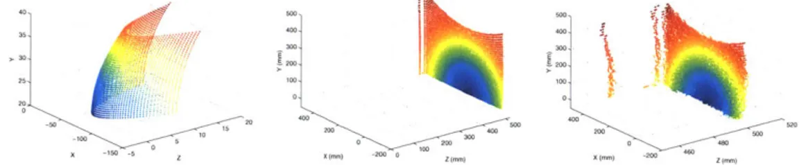
The unfitted data is shown in Figure 3-4a. The fitted projection is shown in Figure 3-4b. The calibration constants obtained give the relation

mm

r = 242.15 i- 718mm (3.1)

mA

The standard deviation of the fitted normal distance is only 4.18mm over a distance of 498mm, or approximately 0.8%. This range is characteristic of the likely ranges sensors would report in an implementation of the array described previously, and the accuracy of the sensor is promising for applications in such a system.

400 . 400

25 50 3 0

-150 0 5 0 200 460 Zm

(a) Unfitted laser sensor cur-(b) Fitted laser sensor output(c) Fitted laser sensor output,

rent scaled

Figure 3-4: Laser sensor ranging a plane. The data is presented as a three dimensional point cloud, with color denoting angle of incidence with the plane

Moreover, the sensor data proved highly repeatable. Repeated measurements at identical angles produced normally distributed data with a standard deviation of just 1.1mm. This suggests that much of the uncertainty in the distribution of points stems from angular dependence; in principle, if we could develop a functional relationship between the angle and the range distortion, we could employ perturbative methods to generate a more accurate measurement of the angle in the sensor array.

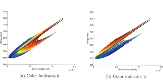
Plotting the measured current against the actual range (as obtained via trigonom-etry) reveals that there is almost no dependence of the error on 0, the angle of rotation about the long dimension of the sensor (Figure 3-5a). However, there is a marked

dependence of error on

#,

the angle of rotation about the short dimension; at large absolute values of

#,

_{the measured range drifts further and further from its actual} value (Figure 3-5b). Unfortunately, attempts to quantify this disturbance were largely unsuccessful; adding first and second order perturbative terms to the function for r

were only capable of reducing its standard deviation by a few microns. The new optimal calibration was found to be

mm r =241.9 i - 716mm - 0.188# + 1.29# (3.2) mA 850- 850 800- 800-750- 750 700- 700 E E 650 650 600- 600-550 550 50040 500 4501 _{5 5.5 6} 4501 6.5 5 5.5 6 6.5

Sensor Output (mA) 5553 _{Sensor Output (nA)}

X 106

(a) Color indicates 0 (b) Color indicates

#

Figure 3-5: Range versus measured current. The solid line is the calibration curve. The new standard deviation of the fitted normal distance was measured as 4.15mm; this improvement is likely too small to be significant, and no gain is likely to be had

by attempting to account for angular effects.

One may question whether some of the error observed in the experiment is endemic to the machine itself, rather than the laser array. While this is certainly possible, it is unlikely; in addition to the manufacturer's claims of accuracy, two simple tests suggest the motion of the machine to be very accurate. First, the machine was able to repeatedly hit a mark on a target wall with the laser beam, even after being taken through its entire range of motion, and even when the wall was a substantial distance

- over twenty feet - away. Second, careful measurements of the motion of the laser

-1000 5 1

-500 0 500 1 000 1500 2;000

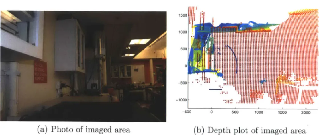
(a) Photo of imaged area (b) Depth plot of imaged area

Figure 3-6: Depth mapping of an area of the lab. Color denotes distance from camera. given. That is to say, when the laser was told to move, for instance, one degree, the observed motion corresponded almost exactly to that predicted by trigonometry. Given this demonstrated accuracy and precision, it seems reasonable to ascribe any error to the laser unit itself, and not the machine.

3.3

Imaging

As an application of the calibrated laser sensor, we use the pan-tilt unit for imaging. This reveals several attributes of the sensor data.

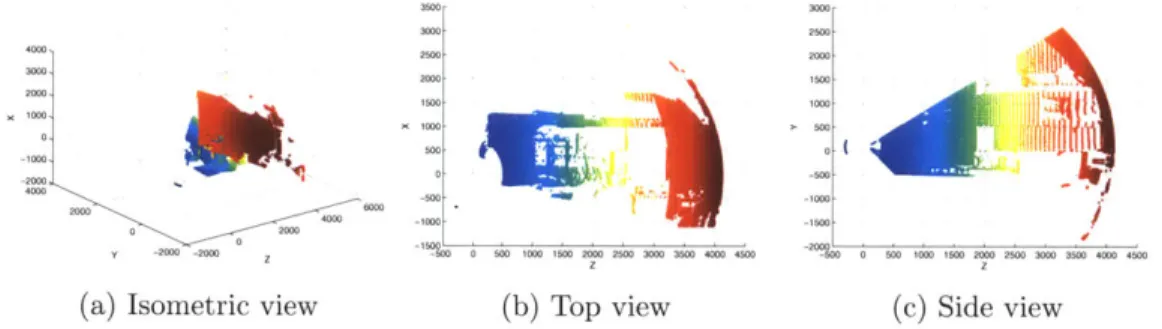
Features can be clearly differentiated at many ranges (on the order of 300mm to 4000mm) in the image in Figure (3-6). For instance, the cupboard and pipes on the left of the photo are visible, as are the drop ceilings and and table on the far right. Accuracy seriously breaks down at longer ranges, however; the red background of the image fails to track the planar shape of the far wall, and is instead roughly dome-shaped, as can be seen in Figure (3-7). This may be due to the exhaustion of the sensor unit's range; the true distance was very nearly the limit of the sensor's advertised 8m range.

4000

4000

Y -200 -200 Z

(a) Isometric view

Iq

-Tpi 500W 0 50W 1000 1500 2 2500 3000 3500 400 4500 (b) Top view ()0 50 100 150 2 250 30 35d 4ve 45 (c) Side view

Conclusion

Both the experimental and theoretical work done here can serve as useful background and groundwork for the construction of a laser array system. The algorithms pre-sented in the first part of this paper are efficient and in some sense optimal; they extract very nearly as much information as can be extracted from the range-finder

data, and perhaps equally important, they can be implemented easily in low-level languages. The most computationally complex step is the inversion of a four-by-four matrix. Moreover, the theoretical framework is scalable and robust, two useful fea-tures in a system of this type; to generate more accurate data, we can simply add more sensors, without doing a significant amount of additional work.

The experimental work offers two key results. First, it generated a calibration curve for the sensors, which was found to be very nearly identical in each of several sensors. This curve will allow for more accurate measurement when the sensors are deployed; without it, we would be forced to estimate a calibration from the manufacturer's data sheets, and given how far off our initial guesses were before calibration, this would certainly result in greatly diminished accuracy. Second, the experiments allowed us to get a gauge on how accurate the sensors are. For instance, we measured experimentally the standard deviation of ranges reported, and found it to be quite small. We also were able to measure things like deviations from linearity in the sensors; results indicated that all higher-order terms and all angular dependence are negligible in the regions of interest. This greatly simplifies the later design of the

sensor arrays, and suggests such a system can be highly accurate.

There are several concerns not addressed in this paper. One key design parameter for the array system will be its throughput. The target application seeks to operate at a command frequency of roughly 100Hz; the array will only be useful if it can operate at similar speeds. While the sensors themselves have the bandwidth to operate at such speeds, the rest of the system needs to be able to keep up. The National Instruments

ADC we used for experiments here - chosen for its compatibility with Labview - would

be far too slow at its 'high resolution' setting, and even its 'high speed' setting may not be fast enough. We did an initial investigation of other ADC chips; while high-resolution, high-bandwidth chips do exist, they tend to be expensive and frequently introduce a large time delay. While this is fine for calibration and measurement, it could be extremely detrimental if it occurs inside a command loop.

Finally, it remains to be studied precisely how to best integrate such an array into a command loop. While the method outlined in Section (2.2) does utilize the redundancy of the array, the inclusion of other sensors, such as gyroscopes or tilt sensors, could augment this method to offer even more redundancy. There exist various ways of measuring tilt and height, each with differing advantages; some have better noise characteristics, some offer faster responses, and some are more consistent. An ideal system would incorporate several types of sensors and synthesize their output to generate superior results. The results of this research clearly indicate, however, that a laser range finder array can and should form an integral part of any such ensemble.