Compact parametric models for efficient sequential decision making in high-dimensional, uncertain domains

Compact Parametric Models for Efficient Sequential

Decision Making in High-dimensional, Uncertain Domains

by

Emma Patricia Brunskill

Submitted to the Department of Electrical Engineering and Computer

Science

in partial fulfillment of the requirements for the degree of

Doctor of Philosophy

at the

MASSACHUSETTS INSTITUTE OF TECHNOLOGY

MASSACHUSETTS INSTITUTE OF TECHNOLOGY

AUG 0

7 2009

SLBRARIES

June 2009

@

Massachusetts Institute of Technology 2009. All rights reserved.

ARCHIVES

Author ..

Department of Electrical Engineering and Computer Science

May 21, 2009

Certified by.

Nicholas Roy

Assistant Professor

Thesis Supervisor

Accepted by..

/

Terry P.Orlando

Compact Parametric Models for Efficient Sequential Decision Making

in High-dimensional, Uncertain Domains

by

Emma Patricia Brunskill

Submitted to the Department of Electrical Engineering and Computer Science on May 21, 2009, in partial fulfillment of the

requirements for the degree of Doctor of Philosophy

Abstract

Within artificial intelligence and robotics there is considerable interest in how a single agent can autonomously make sequential decisions in large, high-dimensional, uncertain domains. This thesis presents decision-making algorithms for maximizing the expcted sum of future rewards in two types of large, high-dimensional, uncertain situations: when the agent knows its current state but does not have a model of the world dynamics within a Markov decision process (MDP) framework, and in partially observable Markov decision processes (POMDPs), when the agent knows the dynamics and reward models, but only receives information about its state through its potentially noisy sensors.

One of the key challenges in the sequential decision making field is the tradeoff between optimality and tractability. To handle high-dimensional (many variables), large (many po-tential values per variable) domains, an algorithm must have a computational complexity that scales gracefully with the number of dimensions. However, many prior approaches achieve such scalability through the use of heuristic methods with limited or no guarantees on how close to optimal, and under what circumstances, are the decisions made by the al-gorithm. Algorithms that do provide rigorous optimality bounds often do so at the expense of tractability.

This thesis proposes that the use of parametric models of the world dynamics, rewards and observations can enable efficient, provably close to optimal, decision making in large, high-dimensional uncertain environments. In support of this, we present a reinforcement learning (RL) algorithm where the use of a parametric model allows the algorithm to make close to optimal decisions on all but a number of samples that scales polynomially with the dimension, a significant improvement over most prior RL provably approximately optimal algorithms. We also show that parametric models can be used to reduce the computational complexity from an exponential to polynomial dependence on the state dimension in for-ward search partially observable MDP planning. Under mild conditions our new forfor-ward- forward-search POMDP planner maintains prior optimality guarantees on the resulting decisions. We present experimental results on a robot navigation over varying terrain RL task and a large global driving POMDP planning simulation.

Thesis Supervisor: Nicholas Roy Title: Associate Professor

Acknowledgments

As I pass out of the hallowed hallows of the infamous Stata center, I remain deeply grateful to those that have supported my graduate experience. I wish to thank my advisor Nicholas Roy, for all of his insight, support and particularly for always urging me to think about the potential impact of my work and ideas, and encouraging me to be broad in that impact. Leslie Kaelbling and Tomas Lozano-Perez, two of my committee members, possess the remarkable ability to switch their attention instantly to a new topic and shed their immense insight on whatever technical challenge I posed to them. My fourth committee member, Michael Littman, helped push me to start thinking about the theoretical directions of my work, and I greatly enjoyed a very productive collaboration with him, and his graduate students Lihong Li and Bethany Leffler.

I have had the fortune to interact extensively with two research groups during my time at MIT: the Robust Robotics Group and the Learning and Intelligent Systems group. Both groups have been fantastic environments. In addition, Luke Zettlemoyer, Meg Aycinena Lippow and Sarah Finney were the best officemates I could have ever dreamed of, always willing to read paper drafts, listen attentively to repeated practice presentations, and share in the often essential afternoon treat session. I wish to particularly thank Meg and Sarah, my two research buddies and good friends, for proving that an article written on providing advice on how to be a good graduate student was surprizingly right on target, at least on making my experience in graduate school significantly better.

Far from the work in this thesis I have been involved in a number of efforts related to international development during my stay at MIT. It has been my absolute pleasure to collaborate extensively with Bill Thies, Somani Patnaik, and Manish Bhardwaj on some of this work. The MIT Public Service Center has generously provided financial assistance and advice on multiple occasions for which I am deeply grateful. I also appreciate my advisor Nick's interest and support of my work in this area.

I will always appreciate my undergraduate operating systems professor Brian Bershad for encouraging me to turn my gaze from physics and seriously consider computer science. I credit he, Gretta Smith, the graduate student that supervised my first computer science research project, and Hank Levy for showing me how exciting computer science could be, and convincing me that I could have a place in this field.

My friends have been an amazing presence in my life throughout this process. Molly Eitzen and Nikki Yarid have been there since my 18th birthday party in the first house we all lived in together. The glory of Oxford was only so because of Chris Bradley, In-grid Barnsley, Naana Jumah, James Analytis, Lipika Goyal, Kirsti Samuels, Ying Wu, and Chelsea Elander Flanagan Bodnar and it has been wonderful to have several of them over-lap in Boston during my time here. My fantastic former housemate Kate Martin has the unique distinction of making even situps seem fun. Chris Rycroft was a fantastic running partner and always willing to trade math help for scones. I've also had the fortunate to cross paths on both coasts and both sides of the Atlantic pond with Marc Hesse since the wine and cheese night when we both first started MIT. There are also many other wonderful individuals I've been delighted to meet and spend time with during my time as a graduate student.

Most of the emotional burden of me completing a PhD has fallen on only a few unlucky souls and I count myself incredibly lucky to have had the willing ear and support of two of my closest friends, Sarah Stewart Johnson and Rebecca Hendrickson. Both have always inspired me with the joy, grace and meaning with which they conduct their lives.

My beloved sister Amelia has been supportive throughout this process and her dry librarian wit has brought levity to many a situation. My parents have always been almost unreasonably supportive of me throughout my life. I strongly credit their consistent stance that it is better to try and fail than fail to try, with their simultaneous belief that my sister and I are capable of the world, to all that I have accomplished.

To my parents and sister

for always providing me with a home, no matter our location, and for their unwavering love and support.

Contents

Introduction

1.1 Framework ...

1.2 Optimality and Tractability . ...

1.3 Thesis Statement ... 1.4 Contributions . ...

1.5 Organization . ...

2 Background

2.1 Markov Decision Processes . ... 2.2 Reinforcement Learning ...

2.2.1 Infinite or No Guarantee Reinforcement Learning 2.2.2 Optimal Reinforcement Learning

2.2.3 Probably Approximately Correct RL 2.3 POMDPs ...

2.3.1 Planning in Discrete-State POMDPs 2.4 Approximate POMDP Solvers ...

2.4.1 Model Structure ... 2.4.2 Belief Structure ... 2.4.3 Value function structure ... 2.4.4 Policy structure ... 2.4.5 Online planning ... 2.5 Summary . ...

3 Switching Mode Planning for Continuous Domains 3.1 Switching State-space Dynamics Models ... 3.2 SM-POMDP ...

3.2.1 Computational complexity of Exact value 3.2.2 Approximating the oj-functions ...

3.2.3 Highest Peaks Projection ... 3.2.4 L2 minimization ... 3.2.5 Point-based minimization ... 3.2.6 Planning ...

3.3 Analysis . ...

3.3.1 Exact value function backups ...

3.3.2 Highest peak projection analysis ...

3.3.3 L2 minimization analysis ... 3.3.4 Point-based minimization analysis .

3.3.5 Computational complexity of backup ope tion operator ...

3.3.6 Analysis Summary . ...

3.3.7 Finding Power: Variable Resolution Exam

function backups

rator when use a I

ple ...

3.3.8 Locomotion over Rough Terrain: Bimodal Dynamics

projec-.

3.3.9 UAV avoidance ... 3.4 Limitations ...

3.5 Summary ...

4 Learning in Switching High-dimensional Continuous Domains

4.1 Background . . .

4.1.1 Algorithm ...

4.2 Learning complexity . . . ... 4.2.1 Preliminaries and framework . . . . . 4.2.2 Analysis . . . . 4.2.3 Discussion ... 4.3 Experiments . ... ... 4.3.1 Puddle World . . . ... 4.3.2 Catching a Plane . . . .... 4.3.3 Driving to Work . . . .

4.3.4 Robot navigation over varying terrain 4.4 Limitations & Discussion . . . .... 4.5 Summary . ...

5 Parametric Representations in Forward Search Planning 5.1 Forward Search POMDP Planning . . . .... 5.2 Model Representation . ...

5.2.1 Hyper-rectangle POMDPs . . . .... 5.2.2 Gaussian POMDPs ...

5.2.3 Alternate Parametric Representations . . . . . 5.3 Planning . ...

5.4 Experiments . . . ...

5.4.1 Boston Driving Simulation . . . .... 5.4.2 Unmanned Aerial Vehicle Avoidance . . . . .

5.5 Analysis . . . ... 5.5.1 Exact Operators . ... 5.5.2 Approximate operators . ... 5.6 Limitations & Discussion ... 5.7 Summary . . . ...

6 Conclusions

6.1 Future Research Possibilities . ... ... 6.1.1 Planning in CORL ...

6.1.2 Learning Types .

6.1.3 Increasing the horizon of search in LOP-POMDP 6.1.4 Model assumptions . ...

6.1.5 Applications . ... 6.2 Conclusion . . . ...

A Theorems from Outside Sources Used in Thesis Results

" ' ' ' 78 80 81 82 82 83 96 97 97 99 101 104 106 107 108 109 113 115 118 120 120 121 121 123 124 125 126 127 130 131 132 132 133 133 133 133 134 135

...

. . °

List of Figures

1-1 Driving example . ... . . . .. ... ... . .. 14

1-2 Tractability, Optimality & Expressive Power ... . . ... . . 17

2-1 Markov transition model ... . . ... 22

2-2 Reinforcement Learning ... ... . .. ... 24

2-3 Function approximation in RL ... . ... . 28

2-4 POMDP transition and observation graphical model ... 31

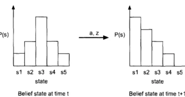
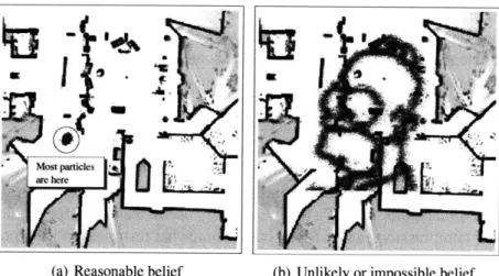
2-5 POMDP Belief States ... . . ... 32

2-6 1-step a-vector example .. . . . . ... ... . 34

2-7 Comparing 1-step a-vectors ... .... 35

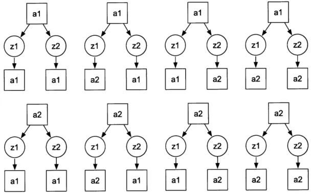
2-8 Conditional policy trees for POMDPs .. ... .. ... .35

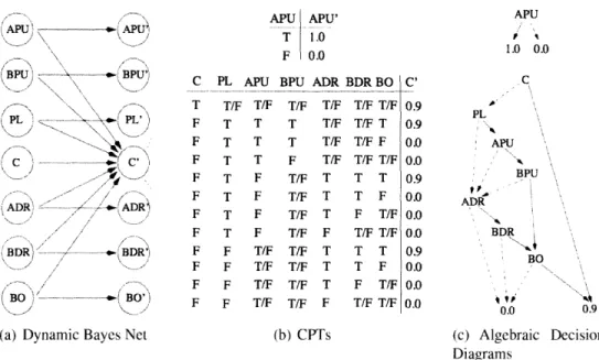
2-9 DBN representations for POMDP models ... .. . . . . . . 38

2-10 POMDP belief compression ... . . 41

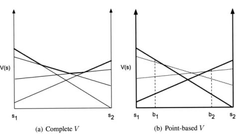
2-11 Point-based value iteration ... . . ... ... 44

2-12 Finite state controller for tiger POMDP .. ... . . . . 46

3-1 Optimality, tractability and expressive power of SM-POMDP .. . . . . 50

3-2 Switching State-Space Models ... ... . . 52

3-3 Example of a mode model p(m ls) ... ... 53

3-4 Sample a-function ... ... . . . .... 57

3-5 Highest peak projection ... . ... . . .. . . . 59

3-6 L2 clustering for projecting the a-function ... 59

3-7 Original and projected a-functions using L2 clustering ... . . . .. . 60

3-8 Residual projection method ... ... .62

3-9 Bimodal dynamics in varying terrain simulation example .. . . . . . .. . 73

3-10 Multi-modal state-dependent dynamics of Junmp action .. . . . . 73

3-1 1 SM-POMDP UAV experiment .. . . . . ... . ... 74

4-1 Expressive power, optimality and tractability of CORL ... . . . . . .. . 79

4-2 Driving to the airport .... . . ... ... . .. . 100

4-3 Driving to work ... ... ... .... . 101

4-4 Car speed dynamics ... ... 102

4-5 CORL driving simulation results ... . . ... ... ... 103

4-6 CORL robot experiment set up ... .... . 105

4-7 Robot experiment rewards ... ... 106

5-1 Optimality, tractability and expressive power of a representative set of POMDP planning techniques. ... . . . 109

5-2 The first step of constructing a forward search tree for POMDP planning. . 111 5-3 Computing state-action values using a forward search tree. . ... 111

5-4 Hyper-rectangle belief update ... ... 116

5-5 Belielf update using hyper-rectangle representation ... 117

5-7 Boston driving simulation ... .. . . . . 121

5-8 Unmanned aerial vehicle domain . ... .... 124

List of Tables

1.1 Decision making problems ... ... 16 3.1 Projection operation comparison for SM-POMDP algorithm ... 69 3.2 Power Supply experiment ... ... 72 3.3 UAV avoidance average cost results: SPOMDP outperforms the linear model. 75 4.1 PuddleWorld results ... .... .... ... 99 4.2 Catching a plane simulation results ... ... 100 4.3 Average reward on episodes 10-50 for the driving to work example. .... 104 5.1 Results for Boston driving simulation ... . 123

The central problem of our age is how to act decisively in the absence of certainty.

Bertrand Russell

Introduction

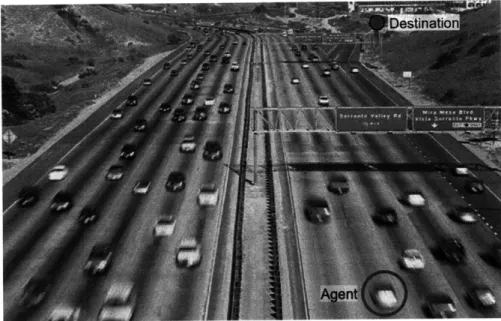
Consider driving on the freeway, trying to reach some far off destination. The state of the environment is large and high-dimensional: the driver must consider the current location of her own car, the location of all the other cars, the weather, if the other car drivers are talking on their cell phones, the time of day, the speed limit, and a number of other variables (or dimensions) each of which can take on a large number of values. At each step the world changes in a stochastic manner: even if the driver knows her own car's behavior, it is likely she can only approximately predict how all the other drivers are going to behave, and it is equally tricky to predict future weather changes, or traffic accidents that may have a significant impact on how the world changes between time steps. In addition, the driver cannot simply teleport to her final destination: she must make a series of decisions in order to try to reach her destination as quickly as possible without colliding with any other vehicles.

This thesis will focus on algorithms to autonomously make a sequence of decisions in such large, high-dimensional, uncertain domains. In particular the work will consider two decision making scenarios. In the first case, imagine that the driver is learning how to drive, or has recently moved to a new city and so is learning the standard traffic behavior of a new area. Imagine also that this learner is equipped with a GPS unit, has the radio on to hear of upcoming traffic delays, construction and weather changes, and has excellent mirrors and cameras that provide her with high quality estimates of all the surrounding cars. This driver is learning the best way to get home given she doesn't know exactly how her car or the dynamics of the world works, but she does have a very good estimate of the current world state at each time step. We will frame this problem as one of learning in fully observable large, high-dimensional Markov decision processes.

Now imagine our driver has passed her driver's test, or has lived in her new city long enough to become well acquainted with the local driving culture and customs. Unfortu-nately one day she loses her GPS unit and her radio breaks. The driver has a good model of how the dynamics of the world works but now the world is only partially observable: the driver can only gain state information through her local car sensors, such as by checking her right side mirror to determine if a car is on her right. When planning her route home, the driver must now consider taking actions specifically to try to gather information about the world state, such as checking whether it is safe to change lanes. This second prob-lem of interest is one of planning in a large, high-dimensional partially observable Markov decision process.

Figure 1-1: Driving to a destination: a large, high-dimensional, uncertain sequential deci-sion making problem.

we have introduced these problems using the particular example of autonomous navigation, sequential decision making in large, high-dimensional, uncertain domains arises in many applications. For example, using robots for autonomous scientific exploration in extreme environments can require examining whether a sample is likely to be interesting, as well as collecting samples believed to be useful, and decisions made must also account for energy and communication constraints (Bresina et al., 2002; Smith, 2007). Similar issues arise in many other robotics problems, including robust motion planning in a crowded museum environment (Thrun et al., 2000) or learning new complicated motor tasks such as hitting a baseball (Peters & Schaal, 2008). Figuring out the right sequence of investment decisions (buying, selling, investing in CDs, etc.) in order to try to retire young and wealthy is another example of sequential decision making in an uncertain, very large domain. Sequential de-cision making under uncertainty frequently arises in medical domains, and algorithms have or are being developed for ischemic heart disease treatment (Hauskrecht & Fraser, 2000), adaptive epilepsy treatment (Guez et al., 2008) and learning drug dosing for anemia treat-ment (Martin-Guerrero et al., 2009). Therefore approaches for making efficiently making good decisions in high-dimensional, uncertain domains are of significant interest.

1.1

Framework

The start of modem decision theory came in the 17th century when Blaise Pascal gave a pragmatic argument for believing in God.1 The key idea behind Pascal's wager was to 1"God is, or He is not... But to which side shall we incline? Reason can decide nothing here... A game is being played.., where heads or tails will turn up. What will you wager? Let us weigh the gain and the loss

evaluate different decisions by comparing their expected benefit. Each decision can lead to one of a number of potential outcomes, and the benefit of a decision is calculated by summing over the probability of each outcome multiplied by the benefit of that outcome. The decision to be taken is the one with the highest expected benefit.

Later Richard Bellman developed the popular Markov decision process (MDP) frame-work that extends this idea of expected benefit to sequential decision making (Bellman, 1957). In sequential decision making a human or automated system (that we refer to as an agent in this document) gets to make a series of decisions. After each decision, the environment may change: a robot may hit a ball, or the driver may take a left turn. The agent must then make a new decision based on the current environment. Sequential deci-sion making immediately offers two new complications beyond the framework illustrated by Pascal's wager. The first is how to represent the environmental changes over time in response to decisions. Bellman's MDP formulation makes the simplifying assumption that the environment changes in a Markovian way: the environmental description after an agent takes an action is a function only of the world environment immediately prior to acting (and no prior history), and the action selected. Second, sequential decision making requires a re-examination of the methodology for choosing between actions. Instead of making deci-sions based on their immediate expected benefit, Bellman proposed that decideci-sions should be taken in order to maximize their long term expected benefit, which includes both the immediate benefit from the current decision, and the expected sum of future benefits. Max-imizing the sum of rewards allows agents to make decisions that might be less beneficial temporarily, such as waiting to make a left hand turn, in order to achieve a larger benefit later on, such as reaching the driver's destination. To compute this quantity, Bellman intro-duced the idea of a value function that represents for each world state the expected sum of future benefits, assuming that, at each time step the best possible decision is made for the resulting state.

One of the limitations of Bellman's approach is that it both assumes that the world models, and the world state are perfectly known. Unfortunately, this is not always the case: it may be hard or impossible to specify in advance a perfect model of a robot arm's dynamics when swinging a baseball bat, an investor may not be able to predict a coming subprime crisis, and a driver may only be able to check one of her mirrors at a time to view surrounding traffic. Problems that exhibit model uncertainty form part of the field of Reinforcement Learning (Sutton & Barto, 1998). Sequential decision making within reinforcement learning is often referred to simply as "learning" since the algorithm has to learn about how the world operates.

In some situations the world state is only accessible through an observation function. For example, a driver with a broken radio and no GPS unit must rely on local observations, such as checking her right mirror, in order to gain partial information about the world state. In order to represent such domains in which the agent receives information about the world state solely through observations, the Markov Decision Process formalism has been extended to the Partially Observable MDP (POMDP) framework (Sondik, 1971). Within the POMDP framework, the history of observations received and decisions made is often

in wagering that God is. Let us estimate these two chances. If you gain, you gain all; if you lose, you lose nothing. Wager, then, without hesitation that He is." Blaise Pascal, Pensdes

Models Known, State Known Models Unknown and/or State

Partially Observed

Single Decision Pascal's Wager

Multiple Decisions Markov Decision Processes Reinforcement Learning,

POMDPs

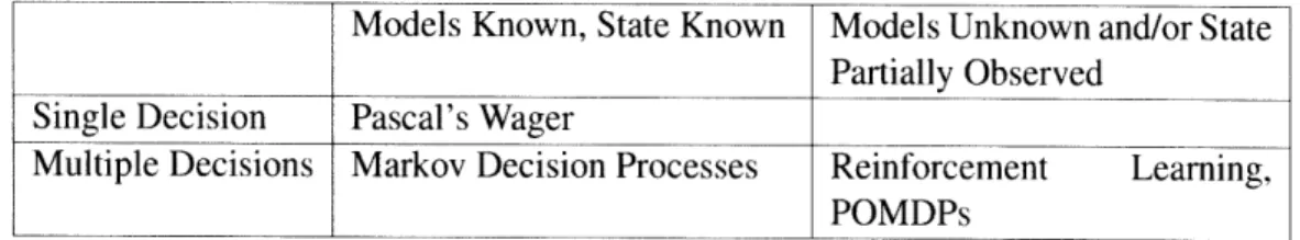
Table 1.1: Overview of some types of decision making under uncertainty problems.

summarized into a probability distribution which expresses the probability of the agent currently being in any of the world states. Since the true world state is unknown, instead this distribution over states is used to select a particular decision, or action, to take at each time step. As in MDPs, we will again be interested in computing a strategy of mapping distributions to decisions, known as a policy, in order to maximize the expected discounted sum of future benefits. Within the POMDP setting we will focus on computing policies when the world models are known: this process is typically known as POMDP planning. Table 1.1 illustrates some of the relationship between different types of decision making problems.

One of the key challenges of sequential decision making in environments with model or sensor uncertainty is balancing between decisions that will yield more information about the world against decisions that are expected to lead to high expected benefit given the current estimates of the world state or models. An example of an information-gathering decision is when a driver checks her blind spot or when a robot arm takes practice air swings to better model the dynamics. In contrast, actions or decisions such as when the driver changes lanes to move towards her destination, or when the robot arm takes a swing at the baseball, are expected to yield a direct benefit in terms of achieved reward. This tradeoff greatly increases the challenge of producing good solution techniques for making decisions.

1.2 Optimality and Tractability

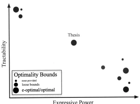
When developing an algorithm for sequential decision making, a key consideration is the evaluation objective: what are the desired characteristics of the final algorithm? As a coarse generalization, the field of sequential decision making under uncertainty within the artificial intelligence community has been predominantly concerned with optimality, tractability and expressive power.

Expressive power refers to the type of dynamics and reward models it is possible to encode using a particular representation. For example, representing the world state by discretizing each variable into a large number of bins, and representing the full state by the cross product of each variable's current bin, is a very expressive model because with a fine enough discretization it can represent almost any possible dynamics or reward model. In contrast, a model which represents the world dynamics as a linear Gaussian, has lower expressive power because it can only represent well a subset of world models, namely those in which the dynamics are linear Gaussian.

.0

Thesis

Optimality Bounds

0

none provided O loose bounds e-optimal/optimal

Expressive Power

Figure 1-2: The three criteria of interest in this document for evaluating sequential decision making under uncertainty algorithms: tractability, optimality and expressive power. Most prior approaches tend to either have large expressive power, but low tractability in large, high-dimensional environments, or good tractability but low expressive power. The thesis provides algorithms with provable guarantees on their optimality which lie in the middle ground of this spectrum between tractability and expressive power.

Typically, one objective comes at the sacrifice of the other, as illustrated graphically in Figure 1-2. The computational cost required to exactly solve a generic discrete-state POMDP problem is computationally intractable for the driving example and other high-dimensional, large domains since the number of discrete states typically increases expo-nentially with the number of dimensions. However, a discrete-state representation may have more expressive power than is necessary to represent the regularities in many large, high-dimensional environments, including the driving example. The linear quadratic Gaus-sian controller (Burl, 1998) achieves high tractability by assuming an identical dynamics model across the state space, but this may be too limited to express some domains of inter-est, such as navigation over varying terrain.

It remains an open challenge to create tractable algorithms that make provably good decisions in a large number of high-dimensional, large domains. Tractability is impor-tant for both learning and planning: if the world models are unknown, the amount of data required to achieve good performance should scale gracefully as the state dimensionality increases. The computational complexity of selecting the right action given known world models (planning) should also scale well in high-dimensional state spaces. We also seek optimality guarantees on the performance of these algorithms. Finally, the representations

used should be expressive enough to adequately capture a variety of environments. Prior approaches are not tractable in high-dimensional, large state spaces, do not provide opti-mality analysis, or are too limited in their expressive power to generalize to some of our problems of interest.

This thesis presents progress towards these goals by using compact parametric functions to represent the world models. Compact parametric functions allow values to be specified over large or infinite domains with a small number of parameters 2 by making assumptions

about the particular shape of the function. Representing world models using compact para-metric functions offers three advantages over prior model representations. First, restricting the expressive power of the representation by limiting the number of function parameters leads to faster generalization during learning: intuitively if there are fewer parameters to learn, then the amount of data required to learn them is reduced. This makes learning in high-dimensional environments more tractable. Second, in certain domains restricting the number of model parameters can reduce the computational complexity of planning since there are less parameters to manipulate and update. Third, hierarchical combinations of compact parametric models, such as switching state models (Ghahramani & Hinton, 2000), provide a significant increase in expressive power with only a linear increase in the number of model parameters.

1.3 Thesis Statement

The central claim of this work is that compact parametric models of the world enable more efficient decision making under uncertainty in high-dimensional, large, stochastic domains. This claim will be supported through the presentation of three algorithms, proofs, and experimental results.

1.4 Contributions

The first contribution of this thesis is the Switching Mode POMDP (SM-POMDP) planner which makes decisions in large (infinite) partially-observable environments (Chapter 3). SM-POMDP generalizes a prior parametric planner by Porta et al. (2006) to a broader class of problems by using a parametric switching-state, multi-modal dynamics model. This allows SM-POMDP to obtain better solutions that Porta et al.'s parametric planner in a unmanned aerial vehicle collisions avoidance simulation, and a robot navigation simula-tion where the robot has faulty actuators. We also empirically demonstrate the benefit of continuous parametric models over discrete-state representations. However, in general the number of parameters required to represent the SM-POMDP models increases exponen-tially with the state dimension, making this approach most suitable for planning in a broad range of low-dimensional continuous-domains.

In large fully-observable high-dimensional environments, a similar parametric model can enable much more efficient learning in continuous-state environments where the

2

Our focus will be on representations where the number of parameters required scales polynomially with the state space dimension.

world models are initially unknown. This is demonstrated in the Continuous-state Offset-dynamics Reinforcement Learning (CORL) algorithm (Chapter 4). We represent the dy-namics using a switching, unimodal parametric model that requires a number of param-eters that scales polynomially with the state dimension. CORL builds good estimates of the world models, and consequently make better decisions, with less data: CORL makes e-close to optimal decisions on all but a number of samples that is a polynomial function of the number of state dimensions. CORL learns much more quickly in high-dimensional do-mains, in contrast to several related approaches that require a number of samples that scales exponentially with state dimension (Brafman & Tennenholtz, 2002; Kearns & Singh, 2002; Leffler et al., 2007b). CORL also has the expressive power to handle a much broader class of domains than prior approaches (e.g. Strehl and Littman (2008)) with similar sample complexity guarantees. Our chosen typed parametric model allows CORL to simultane-ously achieve good expressive power and high learning tractability. We show the typed noisy-offset dynamics representation is sufficient to achieve good performance on a robot navigation across varying terrain experiment, and on a simulated driving task using a dy-namics model built from real car tracking data.

In the final contribution of the thesis, we consider how to plan in large and high-dimensional, partially observed environments assuming the world models are known, and present the Low Order Parametric Forward Search POMDP (LOP-POMDP) algorithm (Chapter 5). Forward search planning is a powerful method that avoids explicitly repre-senting the value function over the full state space (see e.g. Ross et al. 2008a). However, prior methods have typically employed representations that cause the computational com-plexity of the forward search operators to be an exponential function of the number of state dimensions. In LOP-POMDP we use low order parametric models to significantly reduce the computational complexity of the forward search operators to a polynomial function of the state dimension. We present several example parametric representations that fulfill this criteria, and also present a theoretical analysis of the optimality of the resulting pol-icy, as well as the total computational complexity of LOP-POMDP. We demonstrate the strength of LOP-POMDP on a simulated driving problem. In contrast to past approaches to traffic driving (McCallum, 1995; Abbeel & Ng, 2004), this problem is formulated as a global partially-observable planning problem, where the agent must perform local collision avoidance and navigation in order to reach a goal destination. A naive discretization of this problem would yield over 1021 discrete states, which is many orders of magnitude larger than problems that can be solved by offline discrete-state POMDP planners.

Together these three contributions demonstrate that compact parametric representations can enable more efficient decision making in high dimensional domains and also support performance guarantees on the decisions made. These claims are empirically demonstrated on a large driving simulation and robot navigation task.

1.5 Organization

Chapter 2 provides an overview of the related background and prior research. Chapter 3 presents the SM-POMDP algorithm, and Chapter 4 presents the CORL algorithm. The LOP-POMDP algorithm is discussed in Chapter 5. To conclude, Chapter 6 outlines future

Uncertainty and expectation are the joys of life.

William Congreve

Background

Sequential decision making under uncertainty has a rich history in economics, operations research, robotics and computer science. The work of this thesis takes as its starting point the artificial intelligence view of sequential decision making under uncertainty, where the main objective is to create algorithms that allow an agent to autonmously make decisions in uncertain environments.

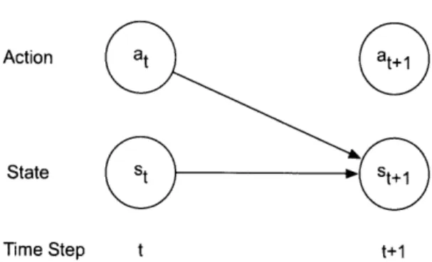
When describing a decision making process, a key component is modeling how the environment (or state) changes over time and in response to actions. Throughout this doc-ument we wil make the common assumption that the way the world state changes at each time step is Markov: namely that the probability of transitioning to the next world state is strictly a function of the current state of the environment and the action chosen, and any prior history to the current state is irrelevant:

p(st+llso, a ,... , , st, at) = p(st+1iist, at).

Figure 2 depicts a graphical model for a Markov transition model.

Decision-making problems which are Markov are know as Markov decision processes (MDPs) and will be discussed shortly. This thesis will focus on two particular problems with the MDP framework. The first problem is that of planning when the models are unknown. This problem arises in a number of applications, including the example presented in the introduction of the driver just learning how to drive, or the driver who has recently moved to a new city and is learning the local traffic customs and patterns. This problem is known as reinforcement learning (RL) since the autonomous agent must, implicitly or explicitly, learn how the world works while simultaneously trying to determine the best way to act to gather reward. In this case the state is assumed to be fully observable. The other contributions of this thesis will consider planning (or control) algorithms for when the models are known but the state is only partially observable, such as when an experienced driver has lost her GPS unit and has a broken radio, and so must therefore rely on local sensing, such as checking her rear-view mirror, in order to estimate the world state.

We will first introduce Markov decision processes formally, and outline a few tech-niques for solving them: such solution algorithms often constitute a subpart of RL or POMDP planning algorithms. We will then discuss reinforcement learning before mov-ing on to the POMDP framework and POMDP plannmov-ing techniques. We do not attempt to cover the vast array of work on sequential decision making under uncertainty, and we will focus our attention on the most relevant related research, while trying to provide enough

Action at

State St St+l

Time Step t t+1

Figure 2-1: Markov transition model context to center our own approaches.

2.1 Markov Decision Processes

Markov decision processes were first introduced by Richard Bellman (1957) and have since been used in a variety of applications, including finance (Schil, 2002), manufacturing pro-cesses, and communications networks (Altman, 2002). In this framework, we assume the existence of an agent that is trying to make decisions, which will be referred to as actions. Formally, a discrete-time' MDP is a tuple (S, A, T,

R,

7) where

* S: a set of states s which describe the current state of the world

*

A: a set of actions a

* p(s' s, a) : S x A x S -+ R is a transition (dynamics) model which describes the

probability of transitioning to a new state s' given that the world started in state s and the agent took action a

*

R : S x A x S - R is a reward function which describes the reward r(s, a, s') the

agent receives for taking action a from state s and transitioning to state s'. In many scenarios the reward will only be a function of s, a or simply the current state s. * EC [0, 1] : _{the discount factor which determines how to weight immediate reward}

versus reward that will be received at a later time step.

The objective of MDP planning is to produce a policy i7 : S - A which is a mapping of states to actions in order to maximize a function of the reward. One very common objec-tive (Sutton & Barto, 1998) is to compute a policy that maximizes the expected discounted sum of future rewards over a time horizon fM (which could be infinite):

arg max E

7

'_R(st+

_1,

(st), st) Iso (2.1)

where the expectation is taken over all potential subsequent states {s, _{... , s"} - _{1} assuming} the agent started in an initial state so. The value of a particular policy 7v for a particular state

'All of the new work presented in this thesis will focus on the discrete time setting and all algorithms should be assumed to be discrete-time algorithms unless specifically stated otherwise.

s, V (s), is the expected sum of discounted future rewards that will be received by starting

in state s and following policy 7 for M steps. In some situations we are interested in the infinite horizon performance (M = oc): the expected sum of discounted future rewards is still finite for infinite horizons as long as the discount factor 7 is less than 1.

The value of a particular policy can be calculated using the Bellman equation which separates the value of a state into an expectation of the immediate received reward at the current timestep, and the sum of future rewards:

V'(s)

=

p(s's, 7i(s))[R(s, 7(s), s') +

2V"(s')]ds'.

(2.2)

If the reward model is only a function of the current state and action selected (r(s, a, s') =

r(s, a)) then the Bellman equation becomes

V'(s) = R(s,

Ts)

+T

f

p(s' s, r(s))Vx(s')ds'. (2.3)

If the number of states is discrete and finite, then writing down the Bellman equation for each state gives a set of IS| (the cardinality of S) linear equations which can be analytically solved to compute the values V'(s) for all s E S. This procedure is known as policy evaluation (Howard, 1960).

Typically we will be interested in finding the optimal policy, rather than only evaluating the value of a particular policy. One common procedure to find the optimal policy is policy iteration. This procedure consists of alternating between evaluating the current policy w

using policy evaluation, and improving upon the current policy to generate a new policy. Policy improvement consists of finding the best action for each state given that the agent takes any action on the first step, and then follows the current policy 7 for all future steps:

7'(s) = arg max p(s' a, s)(R( s. a, s') + V'(s')]ds'. (2.4)

Policy evaluation and policy improvement continue until the policy has converged. The resulting policy has been proved to be optimal (Howard, 1960).

Another popular procedure for computing the optimal policy in an MDP is value itera-tion. Value iteration focuses directly on trying to estimate the optimal value of each state in an iterative fashion, where at each step the previous value function V is used to create a new value function V' using the Bellman operator:

VsV'(s)

=

ma

p(s' a,

s)(R(s, a,

s')

+

V(s'))ds'.

(2.5)

Due to the max over actions, this is not a set of linear equations, and therefore value itera-tion consists of repeatedly computing this equaitera-tion for all states until the value of each state has stopped changing. The Bellman operator is a contraction and therefore this procedure is guaranteed to converge to a fixed point (Banach's Fixed-Point Theorem, presented as Theorem 6.2.3 in Puterman (1994)). Briefly, the Bellman operator can be seen to be a con-traction by considering any two value functions

V

1and V2 for the same MDP and denoting

state

Reward

model?

Figure 2-2: Reinforcement Learning. An agent must learn to act to optimize its expected sum of discounted future rewards without prior knowledge of the world models.

the new value function after the Bellman operator is applied as VI' and V2' respectively. Let

I

Ifl

J denote the max-norm of a function f. Then

1V,'

- V

Io

j0

p(sI

a,

s)(R(s

S')

'

yV(s'))ds'

1 -

p(s'a, s)(R(s, a,

s')

+

-yV

2(s'))ds'

I

= I7

,

p(s' s, a)(Vi(s')

-

V

2

(s))ds'll

-I

V

- V2

which since 7y [0, 1] immediately proves that the Bellman operator is a contraction. The value function at the fixed point of value iteration is guaranteed to be the optimal value function V* (Puterman, 1994). The optimal policy can be extracted from the optimal value function by performing one more backup:

*(s) = argmax p(s'la, s)(R(s, a, s') + yV*(s')]ds'. (2.6)

Both policy iteration and value iteration involve operations with a computational com-plexity that scales polynomially as a function of the size of the state space (O( S21A

I)).

While these approaches work well in discrete-state MDPs with a small number of states, they do not scale well to large or infinite state spaces, such as the driving domain discussed in the introduction. There do exist special cases with analytic solutions, such as the famous linear-quadratic-gaussian (LQG) controller for linear Gaussian dynamics and quadratic re-wards (Burl, 1998), However, the general case of continuous-state MDPs is an active area of research in its own right, and is known to be provably hard (Chow & Tsitsiklis, 1989). Some of the recent advances in this area include work by Kocsis and Szepesviri(2006), Kveton and Hauskretcht (2006), and Marecki and Tambe (2008).

2.2 Reinforcement Learning

In reinforcement learning an agent must learn how to act in a MDP without prior knowledge of the world reward and dynamics models (see Figure 2-2). One of the central challenges in reinforcement learning is how to balance between exploration actions that improve the agent's (implicit or explicit) estimates of the world models, with exploitation actions that are expected to yield high reward given the agent's current estimates of the world models. An agent that exploits too early may make decisions based on estimated world models that are quite different than the true underlying models, and therefore the agent may make suboptimal decisions. On the other hand, an agent that explores forever will never get to use its knowledge to actually select actions that are likely to yield a large sum of rewards, which is the ultimate goal of the agent.

Before we discuss several different approaches to handling exploration and exploitation in reinforcement learning, it is worth noting that there has recently been some interesting developments in the related field of apprenticeship learning (see eg. Abbeel and Ng (2004; 2005)) which take the slightly different approach of assuming that an expert has provided some training examples which an agent can learn from. This approach has had some im-pressive experimental success on helicopter flying and quadruped robot locomotion, and is a promising approach for when some expert training samples are available. In our work we will assume the samples are only generated by the learning agent and so our work falls within the standard reinforcement learning framework.

There are three broad theoretical approaches to handling the exploration/exploitation tradeoff which we now enumerate:

1. Infinite or No Guarantee RL: Place no guarantees on the optimality of the actions

selected, or only guarantee that the actions selected as the number of samples grows to infinity will be optimal.

2. Optimal RL: Optimally balance exploration and exploitation from the first action chosen and guarantee that in expectation the rewards achieved will be the highest possible in the particular environment given the models are initially uncertain. 3. Probably Approximately Correct RL: Allow a finite number of exploratory actions

during which the action selected may have arbitrarily bad reward, but require that the actions selected at all other time steps have a value which is E-close to the value of the optimal action with high probability.

Naturally the second objective seems the most appealing, but there are some significant challenges that mean that it is generally intractable for most domains of interest. We now discuss each approach in more depth.

2.2.1

Infinite or No Guarantee Reinforcement Learning

Many reinforcement learning techniques offer no optimality guarantees on their perfor-mance, or only guarantee that under certain conditions, the actions chosen will be optimal as the number of time steps grows to infinity. For example, a simple popular approach

Algorithm 1 Q-learning Initialize all Q values

Set state s to be drawn from starting state distribution

loop

Generate r, a random number between 0 and 1

if r < E then

a = RandomAction

else

a = argmax, Q(s, a)

end if

Take action a, receive reward r, transition to new state s'

Update the state action value Q(s, a) = (1 - a)Q(s, a) + a(r + argmaxa, Q(s', a')) Update a and E

S = S end loop

is the Q-learning algorithm (Watkins, 1989). In finite state and action spaces, Q-learning typically uses a tabular representation over the estimated values of each state-action pair. After each transition (s, a, s') Q-learning updates the corresponding entry for state s from

which the action a was taken as follows

Q(s,

a) = (1 - a)Q(s, a)

a+

(R + v miax Q(.s', a)) (2.7) where R is the reward received after taking action a from state s and transitioning to state

s', and a is a learning parameter which controls how much to alter the current state-action

estimates. These estimated

Q

values are used to select actions at each time step. There are a number of action-selection methods possible, but a popular approach is known as 6-greedy: at each time step the agent selects the action which maximizes Q(s, a) with probability 1 -E

and otherwise selects an action at random. Algorithm 1 displays this version of Q-learning. If c is decayed over time such that there is always some probability of exploration, and the learning parameter a is reduced by no larger than a factor of 1/t2 as the number of time steps t increases, then Q-leaming is guaranteed to converge to the optimal policy as the number of samples grows to infinity.

Though appealing in its simplicity and computational speed per update, Q-learning typically exhibits extremely slow convergence to a good policy, in large part because at each step only a single state-action pair is updated. For example, if an agent finally found a location with an enormous cookie, only the prior state would have its value updated to reflect the benefit of that action: all other states leading up to the cookie would still have their original values. It can therefore take a long time for changes in the state-action values

to propagate back to precursor states.

In addition, when the number of states is extremely large or infinite, such as in the driving example, the standard tabular representation of the state-action values will not be possible. The state space can be discretized to an arbitrary resolution and standard Q-learning can be applied to this discrete representation. Such an approach has a high degree

of expressive power, since any potential dynamics or reward model can be represented with an arbitrary accuracy if a sufficiently fine grid resolution is employed. The resolution used does not affect the per-step computational cost in Q-learning, since Q-learning only updates a single state-action tuple at each time step. In this sense Q-learning is quite com-putationally tractable for large environments. However its slow convergence becomes even more exaggerated as the state space gets larger, making its learning time intractable in large environments.

A common alternate approach to discretization in large environments is to use some type of function approximation in order to estimate the value function over the large or continuous state space. Sutton and Barton (1998) provide an overview of some of these ap-proaches. The majority of these approaches provide no formal guarantees on the optimality of the actions selected. Indeed, even in the limit of an infinite number of samples, some of these methods will not even converge to a single policy, as demonstrated by Baird (1995)

and Boyan and Moore (1995). Figure 2-3 presents an early example from Boyan and Moore that demonstrates the divergence of the value function on a (now) standard reinforcement learning problem, where linear weighted regression is used as a function approximator. However, Gordon (1995) proved that if the function approximator is an averager, which means that the distance between two approximated points is always smaller than the orig-inal distance between the two points, then reinforcement learning using that function ap-proximation is guaranteed to converge. In parallel Tsitsiklis and Van Roy (1996) proved similar results about function approximators satisfying what they called interpolative repre-sentations. Note that these results guarantee that using these function approximators during reinforcement learning will allow the computed policy to eventually converge, but do not guarantee the resulting policy is optimal.

Most more recent RL approaches are guaranteed to converge, but without necessarily providing guarantees on the resulting optimality of the solution. This is often an issue with function approximation techniques since the particular function used to approximate the value function constrains the space of representable value functions. If the true op-timal value function does not lie in the class of functions used to approximate the value function, it is hard to estimate the resulting error. However, a number of these approaches have good empirical performance and are applicable to a large number of domains (they have high expressive power). For example, Least Squares Policy Iteration (Lagoudakis & Parr, 2003) has good empirical performance but no theoretical guarantees on the pol-icy optimality. There has also been some interesting work in using Gaussian Processes in continuous-state and action reinforcement learning (Engel et al., 2003; Engel et al., 2005; Rasmussen & Kuss, 2004; Deisenroth et al., 2008). One of the interesting advantages of Gaussian Processes is that they automatically encode the degree of uncertainty on the resulting value function estimates, which can be potentially used when selecting actions during exploration. Gaussian Processes are a nonparametric approach and as such have a high degree of expressive power, since they can use represent any function output by the sampled data. However, in general they require that all the data is stored, which means their computational tractability in large domains with long horizons is limited. They also do not provide theoretical guarantees on the resulting actions selected.

Jong and Stone (2007) recently presented Fitted R-max, an approach that can learn in continuous environments which assumes that the dynamics model between nearby states

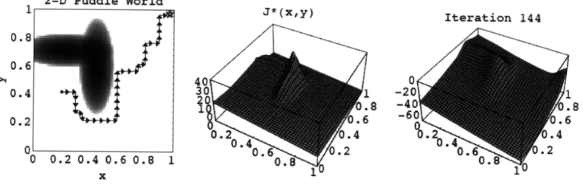
2-D Puddle World 1 J*(x,y) _{Iteration 144} 0.8 0.6 0. 40 0 0.4 _{301 -20 1} .8 -40 .8 2.6 -60 0.6 0.2 T 0.2 4.4 % .4 0 0.6 .2 0.6 .2 0 0.2 0.4 0.6 0.8 1 0.8 0.8 1 1

Figure 2-3: (Reproduced with permission from Boyan and Moore (1995), figure 4). An ex-ample where a standard function approximator, local weighted regression, combined with dynamic programming on a continuous-state problem, causes the value function to diverge. The state space is shown on the left: it is a navigational problem where an agent must learn to avoid the oval puddles and travel to a goal in the right upper corner. The middle figure shows the optimal value function and the right figure shows the approximate value func-tion after 144 iterafunc-tions. One of the interesting points about this example is that although linear weighted regression (LWR) can be used to provide a very good approximation to the optimal value function, if LWR is used to approximate the value function during value iteration, it causes the value function to diverge.

is similar, This allows Fitted R-max to learn more quickly in continuous environments by explicitly assuming a certain amount of generalization between states. Their experimental results were encouraging in low-dimensional environments. However, the amount of sam-ples needed for learning would typically scale exponentially with the state-space dimension since Fitted R-max is an instance-based approach. Therefore, while their approach can rep-resent a large class of problems, meaning that it has a high degree of expressive power, it is not computationally tractable in large domains, and it does not provide formal optimality guarantees.

Recent work by Peters and Schaal (2008) uses a policy gradient approach in which the policy is slowly modified until a local optimum is reached. Their approach works well for allowing a seven degree of freedom robot to learn how to hit a baseball, an impressive demonstration of tractability. However the approach is not guaranteed to find a global optimum.

2.2.2

_{Optimal Reinforcement Learning}

The second potential objective in balancing exploration and exploitation is to attempt to optimally balance between the two from the first action. Most such approaches frame rein-forcement learning within a Bayesian perspective, and consider a distribution over possible model parameters. As the agent acts, receives rewards, and transitions to new states, the dis-tribution over model parameters is updated to reflect the experience gathered in the world. When selecting actions, the agent considers the distribution over model parameters, and

selects actions that are expected to yield high reward given this distribution: such actions could either be information gathering/exploratory or exploitative in nature. In particular, Duff (2002) and a number of other researchers have framed the problem as a partially ob-servable Markov decision process (POMDP) planning problem. We will discuss POMDP planning in detail later in this chapter, but in this context the model dynamics and reward parameters are considered to be hidden states, and the agent maintains a belief over the distribution of potential values of these hidden parameters. In Bayesian RL the bulk of the computational effort is to compute a plan for the POMDP, typically in advance of acting in the real world. This plan essentially specifies the best action to take for any distribution over model parameters, or belief, the agent might encounter. When the agent is acting in the real world, the agent must simply update these distributions (known as belief updating) at each time step to reflect the transition and reward it just experienced, and then use these distributions to index the correct action using the previously computed plan.

One of the challenges in this style of approach is that even if the states in the MDP are discrete, the transition parameters will typically be continuous-valued. Poupart et al. (2006) show how the belief over the hidden model parameters can be represented as a product of Dirichlets: the Dirichlet distribution is the conjugate prior for the multinomial distribution. The authors then prove that the POMDP planning operators can be performed in closed form, and that the value function is represented as a set of multivariate polynomials. The number of parameters needed to represent the value function increases during planning, and so the authors project the updated value function to a fixed set of bases iteratively during the computation. Rather than re-projecting the value at each step, the authors transform the problem to a new altered POMDP over a different set of bases. This greatly reduces the computational load, which allows BEETLE to scale to a handwashing task motivated by a real application, highlighting its computational tractability and expressive power. However, it is unclear how much error is caused by the bases approximation or how to select bases to reduce the approximation error, and the final algorithm does not have bounds on the resulting actions selected.

Castro and Precup (2007) also assume a fully observed discrete state space with hid-den model parameters but represented the model parameters as counts over the different transitions and reward received, thereby keeping the problem fully observable. Doshi et al. (2008) consider a Bayesian approach for learning when the discrete state space is only partially observable. Both of these approaches have good expressive power but will only be tractable in small environments. Also, both are approximate approaches, without formal optimality guarantees on the resulting solution.

Both Wang et al. (2005) and Ross et al. (2008a) present Bayesian forward-search plan-ners for reinforcement learning (RL) problems. Despite the useful contributions of Wang et al. and Ross et al., in both cases the work is unlikely to be computationally tractable for large high-dimensional domains. For example, Ross et al. used a particle filter which has good performance in large, low-dimensional environments, but typically requires a number of particles that scales exponentially with the domain dimension. Like the prior Bayesian approaches outlined, the work of Wang et al. and Ross et al. make few assumptions on the structure of the underlying model structure (so they have good expressive power) but they do not provide guarantees on the optimality of the resulting solutions, and it is unclear how well these approaches will scale to much larger environments.

All the approaches outlined face inherent complexity problems and produce algorithms that only approximately solve their target optimality criteria. Therefore, while the Bayesian approach offers the most compelling objective criteria, to our knowledge there do not yet exist algorithms that succeed in achieving this optimal criteria.

2.2.3

Probably Approximately Correct RL

The third middle ground objective is to allow a certain number of mistakes, but to require that the policy followed at all other times is near-optimal, with high probability. This ob-jective is known as probably approximately correct (PAC). Another very recent and slightly more general objective is the Knows What it Knows (KWIK) learning framework which can handle adversarial environments (Li et al., 2008). Due to the more extensive literature on PAC RL we will focus our discussion on the PAC RL formalism.

The tractability of PAC RL algorithms is typically designated as learning complexity, and consists of sample complexity and computational complexity (Kakade, 2003). Com-putational complexity refers to the number of operations required at each step in order for the agent to compute a new action. Sample complexity refers to the number of time steps at which the action chosen is not close to optimal.

PAC RL was introduced by Kearns and Singh (2002) and Brafman and Tennen-holtz (2002) who created the E' and R-max algorithms, respectively. These algorithms were guaranteed to achieve near optimal performance on all but a small number of sam-ples, with high probability. R-max and E3 were developed for discrete state spaces, and their sample and computational complexity is a polynomial function of the number of dis-crete states. These algorithms can also be applied to continuous state spaces by discretizing the continuous values. However, the R-max and E3 algorithms assume that the dynamics model for each state-action tuple is learned independently. Since each state-action can have entirely different dynamics, this approach has a high expressive power, but as there is no sharing of dynamics information among states, it has a very low level of generaliza-tion. This causes the algorithms to have an extremely large sample complexity in large environments, causing them to have low tractability. In contrast, the work of Strehl and Littman (2008) and the classic linear quadratic Gaussian regulator model (see Burl, 1998) assume that the dynamics model is the same for all states, greatly restricting the expressive power of these models in return for more tractable (fast) learning in large environments.

Kearns and Koller (1999) extended E3 to factored domains and proved that when the dynamics model can be represented a dynamic Bayesian network (DBN), the number of samples needed to achieve good performance is only a polynomial function of the number of DBN parameters. Their approach slightly limits the expressive power of the E3 algo-rithm to a smaller subclass of dynamics models, but makes a significant improvement in tractability, while still providing formal theoretical guarantees on the quality of the result-ing solution. However, the authors assume access to an approximately optimal planner for solving the resulting MDP but do not provide a particular planner that fulfills their assump-tions. Though the algorithm has attractive properties in theory, no experimental results were provided.

Another approach that explores the middle ground between expressive power and (sam-ple com(sam-plexity) tractability is Leffler et al. (2007b)'s work on domains in which the