MODEL-GENERATED VERSUS RADAR-OBSERVED
by
JUDSON EDWARD STAILEY B.S.C.E., The Ohio State
(1971)
MASSA
University
SUBMITTED IN PARTIAL FULFILLMENT OF THE REQUIREMENTS FOR THE DEGREE OF MASTER OF SCIENCE
at the
CHUSETTS INSTITUTE OF TECHN May, 1978
OLOGY
Signature of Author... Department of Meteorology; May 24, 1978.
Certified by... Thesis Supervisor.
Accepted by...
Lindgren
Chairman,
Departmental CommitteeMASSACHUSETTS INSTITUTE on Graduate Students. OF TECHNOLO6Y
JUL
2 7 1978
COMPARISON OF PRECIPITATING CUMULUS CELLS: MODEL-GENERATED VERSUS RADAR-OBSERVED
by
JUDSON EDWARD STAILEY
Submitted to the Department of Meteorology on 24 May 1978 in Partial Fulfillment of the Requirements for
the Degree of Master of Science
ABSTRACT
The purpose of this study was twofold: to evaluate the ability of a circularly symmetric two-cylinder model of a precipitating cumulus cell to simulate radar-observed cells, and to ascertain to what accuracy the model input variables need to be known to obtain realistic results.
Data from GATE were employed because of their availability and cover-age and because the tropical atmosphere during the experiment contained relatively little vertical wind shear. Cells organized into two types of mesoscale features, a line and a cluster, were simulated. Because of the variability observed in the cell characteristics, the mesoscale
features were idealized into geometrically simple configurations of "representative" cells. The representative cells were geometrically com-patible with the model and had dimensions based on the average sizes of observed cells. The size of the model inner cylinder, assumed to be the region of active convection, was estimated from the areas of observed reflectivity cores. The size of the outer cylinder, analogous to the environment of the cells, was estimated from distances between cells in
the mesoscale features. This idealization process produced what appeared to be realistic dimensions.
Vertical profiles of temperature and relative humidity were also
needed forinitialization. A large sample of observed profiles was
ideal-ized by a method which retained the main characteristics of the profiles while smoothing the minor variations. The idealized relative humidity
profiles fell into three distinct types, the distribution of which varied with the synoptic situation. Variations in the idealized temperature
profiles were small and not systematic.
The effectiveness of the model in simulating observed cells was in-vestigated by comparing observed with model cell heights, maximum reflec-tivities, and heights of the reflectivity maxima. When initialized appro-priately, the model produced cells which appeared to be remarkably similar to observed cells. Although cell dimensions were notunimportant, the rela-tive humidity profile exerted the greatest influence on model cell growth,
Open-atmosphere humidity profiles were found to be too dry to support vigorous convection. Realistic cells were generated when the humidity was increased under the assumption that the cells were growing in a mesoscale region which was more moist than the open atmosphere.
Calcu-lations showed that convective activity could contribute to the humidi-fication of the open atmosphere, but this contribution was not sufficient to alter the rilative humidity profile to the point where realistic cells could be simulated. Further humidification via mesoscale ascent was necessary.
The need for taking into account the effects of mesoscale processes is discussed, and methods for doing so are suggested. The need for the addition of a realistic boundary layer is discussed. The further addi-tion of a less artificial initiating impulse coupled with the structure and properties of the boundary layer is suggested.
ACKNOWLEDGEMENTS
The author would like to express his sincere gratitude to Dr. Peter Yau, who designed the model tested in this thesis, took time to acquaint the author with the model, and endorsed this study, Apprecia-tion is also expressed to Dr. Pauline M. Austin, who supervised the research and writing of this thesis. Without her patience, encourage-ment, and expert advice, this thesis would not have been written,
Mr. Frank Marks and Dr. Speed Geotis made themselves available for numerous discussions related to tropical meteorology, the GATE program, and the radar data. Mr, William Silver and Mr. Alan Siggia assisted in computer programming.
The author also thanks his wife, Laura, for proofreading the thesis and for the continued love and understanding she has provided.
Finally, the author is indebted to the Air Force Institute of Technology, which made this research possible, and to Capt. Harry Hughes,
TABLE OF CONTENTS TITLE 1 ABSTRACT 2 ACKNOWLEDGEMENTS 4 TABLE OF CONTENTS 5 LIST OF TABLES 7 LIST OF FIGURES 8
CHAPTER ONE. INTRODUCTION 10
1.1 Background - 10
1.2 Statement of Problem 12
CHAPTER TWO. DESCRIPTION OF MODEL 14
2.1 Microphysical Processes 14
2.2 Model Formulation and Dynamics 15
2.3 Model Input Variables 16
2.3.1 Meteorological Variables 17
2.3.2 Numerical Variables 21
2.4 Model Output Variables 21
CHAPTER THREE. SOURCES OF DATA AND METHODS OF ANALYSIS 23
3.1 The Source of the Data 23
3.2 Analysis of Synoptic-Scale Data 25
3.3 Radar Data 28
3.3.1 Source 28
3.3.2 Handling 28
3.3.3 Analysis 29
3.3.4 Idealization 34
3.3.4.1 Determination of Input Variables. 35 3.3.4.2 Determination of Cell Characteristics for 37
Comparison of Observed with Model Cells
3.4 Upper Air Data 40
3.4.1 Source 40
3.4.2 Handling 40
CHAPTER FOUR. SIMULATION OF CONVECTIVE CELLS IN A LINE 42 4.1 The Line and its Environment -- Observed and Idealized 42
4.1.1 Description of the Line and its Environment 42 4.1.2 Idealization of the Line and its Environment 43
4.1.2.1 Idealization of the Line 43
4.1.2.2 Idealization of the Environment 51
4.2 Experaments 62
4.2.1 Experiments 1-7, Simulation of Cells in the Line 62 4.2.2 Experiments 8-12, Humidification of Dry Layer by 74
Convective Activity
4.2.3 Experiments 13-15, Simulation of a Mesoscale Process 78 4.2.4 Comparison of Model Output to Observed Data 86
4.3 Summary 94
CHAPTER FIVE. SIMULATION OF CELLS IN A CLUSTER 95
5.1 The Cluster and its Environment -- Observed and Idealized 95 5.1.1 Description of the Cluster and its Environment 95 5.1.2 Idealization of the Cluster and its Environment 97
5.1.2.1 Idealization of the Cluster 97
5.1.2.2 Idealization of the Environment 101
5.2 Experiments 106
5.2.1 Experiments 16-19, Simulation of Cells in the Cluster 108 5.2.2 Experiments 20-23, Humidification of Dry Layer by 113
Convective Activity
5.2.3 Comparison of Model Output to Observed Data 122
5.3 Summary 127
CHAPTER SIX. ASSESSMENT OF RESULTS 128
LIST OF TABLES
Table Page
4.1 Results of the idealization of the line. 49,50 4.2 Distribution of soundings by wave sector and day, 52 4.3 Mean values of characteristic features of relative 54
humidity profiles.
4.4 Distribution of relative humidity sounding types 57 by wave sector.
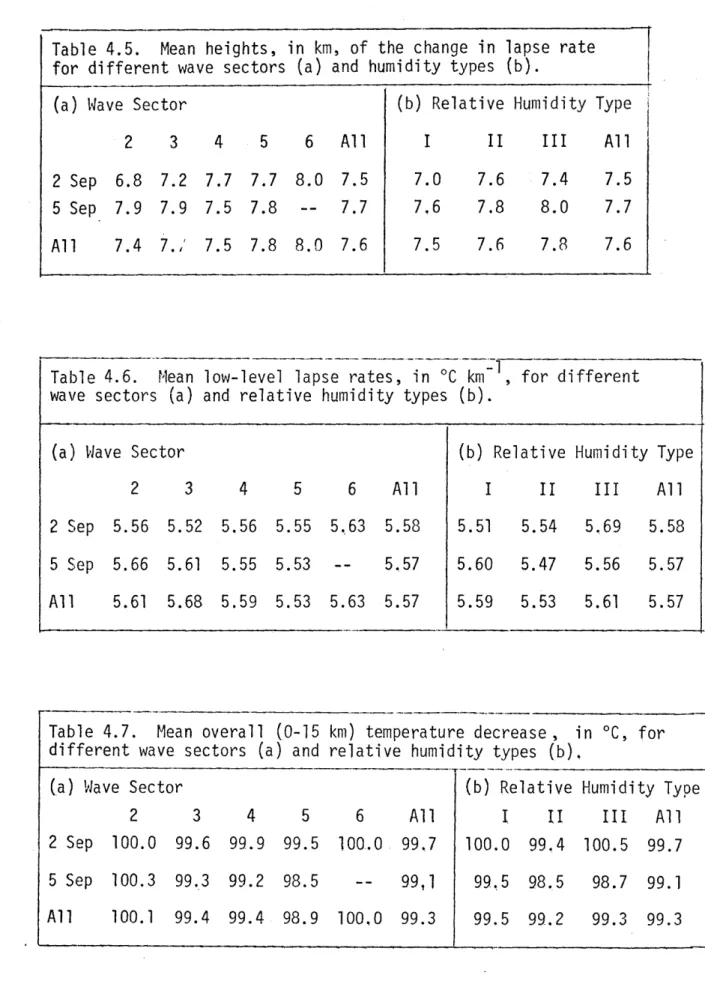
4.5 Mean heights, in km, of the change in lapse rate 60 for different wave sectors and humidity types.
4.6 Mean low-level lapse rates, in *C km~1, for 60 different wave sectors and relative humidity types.
4.7 Mean overall (0-15 km) temperature decrease, in *C, 60 for different wave sectors and relativy humidity types.
4.8 Results of Xl and X8-X12. 75
4.9 Important input variables for X1-X15. 82
4.10 Characteristics of model cells from X1-X15. 83 4.11 Distribution of radar-observed and model (X3) heights 91
of maximum reflectivity,
5.1 Results of idealization of cluster. 102
5.2 Mean values of characteristic features of the idealized 104 relative humidity profiles.
5.3 Mean values of characteristic features of temperature 107 profiles for the cluster.
5.4 Results of X16 and X20-X23. 116
5.5 Important input variables for X16-X23. 120 5.6 Characteristics of model cells from X16-X23. 121
5.7 Distribution of radar-observed vs. model (X18) heights 126 of maximum reflectivity.
Figure 3.1 3.2 3.3 3.4 4.1 4.2 4.3 4.4 LIST OF FIGURES
The GATE ship arrays during Phase III.
Illustration of a GATE wave and its division into sectors.
Example of a CAPPI radar map.
Example of the use of a CAPPI radar map to identify cells and define their updraft areas.
Convective line at 0830Z as seen by radar aboard the Gilliss.
Schematic representation of the idealization process for the line.
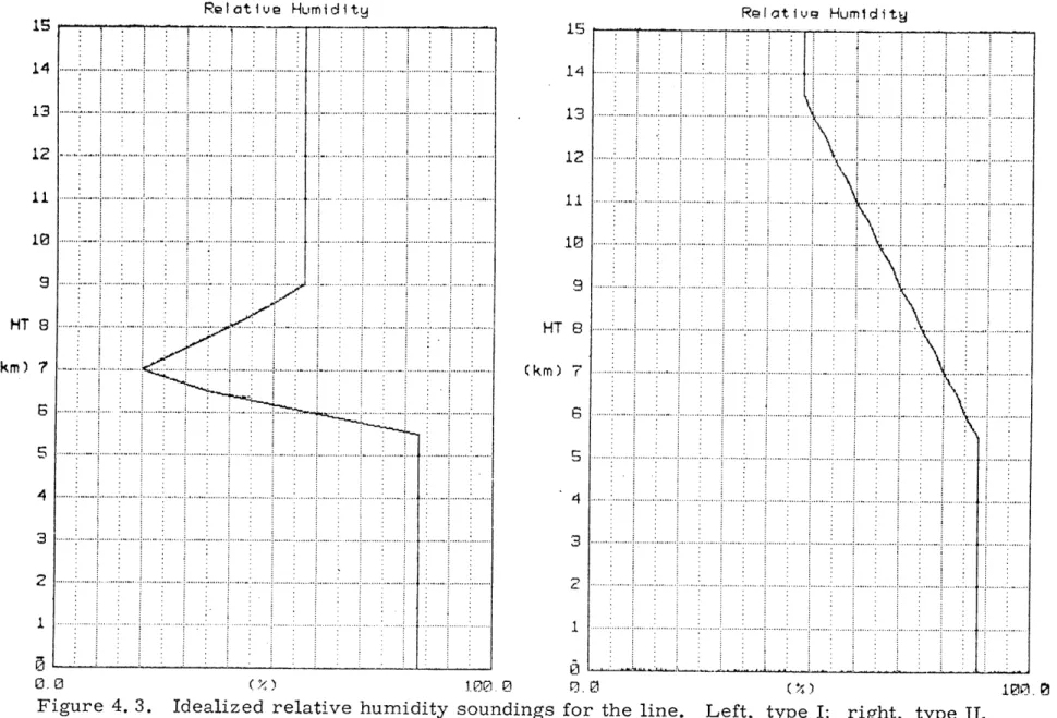
Idealized relative humidity soundings for the line. Sounding used in experiment 1.
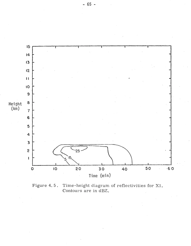
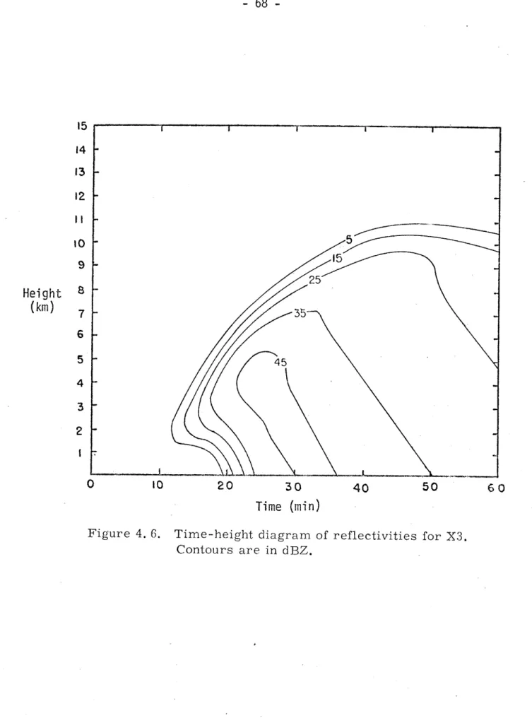
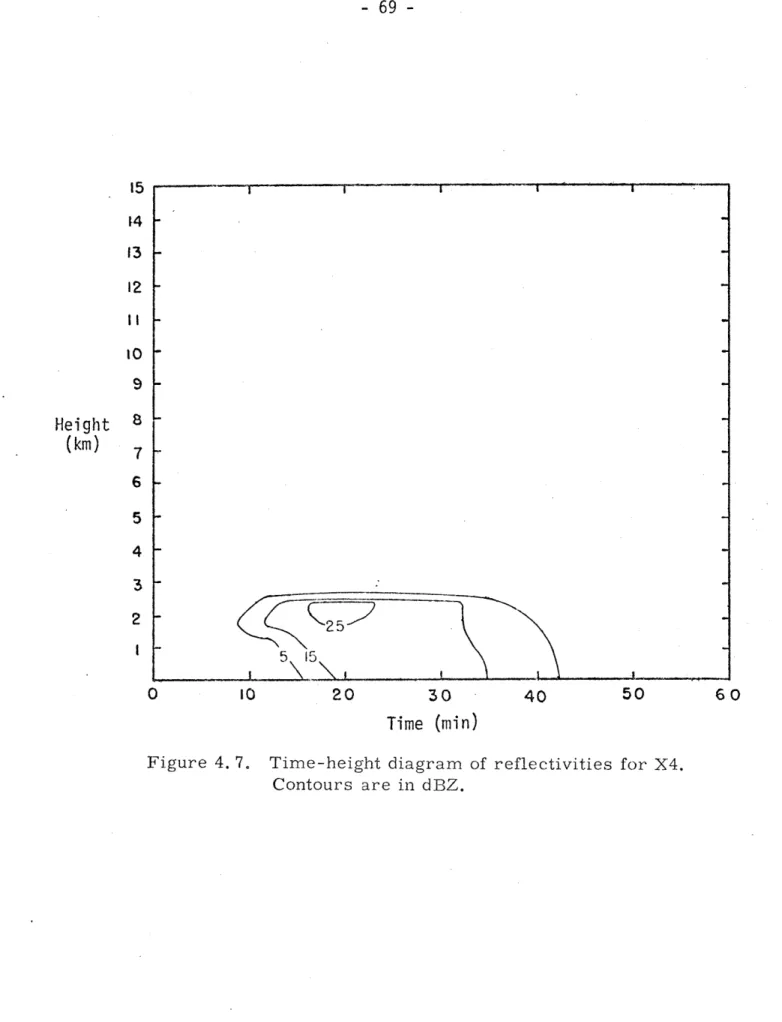
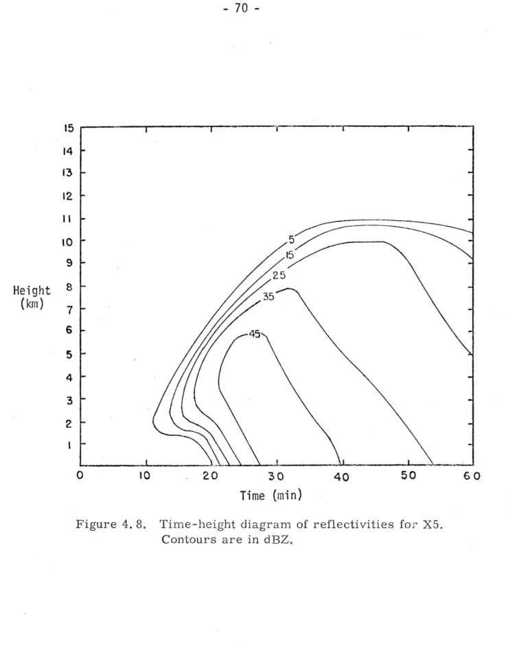
Time-height diagram of reflectivities for Xl. Time-height diagram of reflectivities for X3. Time-height diagram of reflectivities for X4. Time-height diagram of reflectivities for X5. Time-height diagram of reflectivities for X6. Time-height diagram of reflectivities for X7. Successive relative humidity profiles.
Time-height diagram of reflectivities for X13. Time-height diagram of reflectivities for X14. Time-height diagram of reflectivities for X15. Max-tops radar map of line at 0830Z.
Model and observed spectra of maximum reflectivity. Observed and model rainfall rates.
4.5 4.6 4.7 4.8 4.9 4.10 4.11 4.12 4.13 4.14 4.15 4.16 4.17 Page 24 26 30 33 44 47 55,56 64 65 68 69 70 72 73 76,77 80 84 85
Figure Page 5.1 Cluster at 1629Z as seen by radar aboard the Gilliss. 96 5.2 Schematic representation of the idealization process 100
for the cluster.
5.3 Relative humidity profile idealized from all the data 105
for the cluster.
5.4 Sounding used in experiment 16, 109
5.5 Time-height diagram of reflectivities for X16. 111 5.6 Time-height diagram of reflectivities for X17. 112
5.7 Time-height diagram of reflectivities for X18. 114 5.8 Time-height diagram of reflectivities for X19. 115 5.9 Successive relative humidity profiles. 117,118 5.10 Model and observed spectra of maximum reflectivity, 124
CHAPTER ONE
INTRODUCTION
1.1 Background
It is generally recognized that moist convection plays an impor-tant role in vertical heat and moisture transport. Through this role, it is believed to have far-reaching effects on synoptic and global circula-tions (see, e.g. Charney and Eliassen, 1964; Gray, 1973). These effects cannot be completely understood, however, until the nature and magnitude
of cumulus transports can be determined with a reasonable degree of accur-acy. Because of the small scale of cumulus cells and their complexity,
it is extremely difficult to measure directly their transport of heat, moisture, and other qualities, Indirect methods of determining cumulus
transports using radar data (Austin and Houze, 1973) or diagnostic studies of large-scale variables (Arakawa and Schubert, 1974) have been devised, but they provide only crude estimates,
One tool which can aid the meteorologist in investigating cumulus transports is the cumulus cell model. Cell models have been designed to serve a number of purposes (investigation of microphysical or dynamical processes, aids in weather modification experiments, etc.). Some of these models might be suitable for use in cumulus transport studies provided
that they are capable of simulating observed cells with a sufficient
degree of detail. Comparisons of cells generated by the more theoretically oriented models with observed cells have usually been made in the most general way, involving only the concern that the model cell resemble a
(i.e. any) cumulus cell (see, e.g. Orville and Sloan, 1970, who considered
the configuration of orographically induced cells), In
other studies
(e.g. Heinstein, 1970), in
which particular observed cells were modeled,
qualitative comparisons have been made between the general appearance of
major features in
the modeled and observed cells. The quantitative
com-parisons that have been made (e.g. Sax, 1969, who compared computed with
observed cell heights} were not made in
sufficient detail to elicit
confi-dence in
the models' ability to simulate important cumulus processes.
The main difficulty in
making comparisons has stemmed from the
lack of important processes or properties which could be both observed in
a real cell and calculated in
a model with sufficient accuracy and
reso-lution to allow a reasonably accurate comparison. Yau (1977) has
contri-buted to the solution of this problem by devising a microphysical
para-meterization which allows for the natural development of drop size spectra
and thus the calculation of realistic radar reflectivities. These
reflec-tivities can be compared with reflecreflec-tivities observed within real cells
by radar. Yau incorporated his microphysical parameterization into a
fairly sophisticated two-cylinder model in
which an inner cylinder
repre-sents a cumulus cell and a surrounding outer cylinder reprerepre-sents the
environment of the cell, This type of formulation, while being reasonably
well suited for investigating cumulus transports, requires less computation
than the more complex two-dimensional models of, for example, Soong and
Ogura (1976). This computational simplicity permits relatively extensive
experimentation to be carried out.
1.2 Statement of*Problem
In spite of the advantages of Yau's model, it is, compared to the real world, highly simplified. In order to assess its usefulness for com-puting vertical transports, it is desirable to determine how well it simu-lates real cells. Toward this objective, this study will compare cells generated by the model with cells observed by radar. A secondary objective is to determine specifically what characteristics of cells and the atmo-sphere in which they are occurring need to be known, and to what accuracy they need to be known, in order to achieve realistic simulations from the model.
The model will be initialized with horizontal cell dimensions estimated from radar data and with environmental temperature and relative humidity profiles determined from rawinsonde soundings, Comparisons will be made between radar reflectivities generated by the model and those ob-served by radar. The data will be drawn from the GARP* Atlantic Tropical Experiment (GATE). This data set was chosen for its availability and ex-cellent coverage and because the tropical atmosphere has relatively little vertical wind shear, a property which cannot be taken into account by the axisymmetric cell model.
In Chapter 2, the model microphysics, dynamics, and general formu-lation are briefly described. The input variables are discussed and the results of Yau's sensitivity tests on those variables are presented.
Values of input variables which will remain constant throughout this study and the rationale behind their choice will be given.
The data are discussed in Chapter 3. A brief description of GATE is given after which the sources, handling, and analysis of the data are described. The need for idealizing the data to provide "representative" cell dimensions and soundings is discussed and the idealization process is described. Methods for comparison of model-generated with radar-observed cells are presented.
Two types of situations are considered. Qne is a well-organized and well-developed line of convective cells, a configuration which is typical of tropical disturbances. Experiments and comparisons for this situation are presented in Chapter 4, The second type of situation, a cluster of cells which occurred during a relatively undisturbed period, is considered in Chapter 5.
Conclusions drawn from the experiments and recommendations for future use of the model are presented in Chapter 6.
CHAPTER TWO
DESCRIPTION OF MODEL
The model being evaluated in this thesis was designed by M.K. Yau (1977) to allow investigation of the interaction of dynamical and
micro-physical processes in precipitating cumulus clouds. In this chapter, a
brief description of the important characteristics and properties of the model is given.
2.1 Microphysical Processes
The microphysical processes were designed to be a compromise
between the explicit calculation of diffusional growth of drops and of
stochastic collection processes and the simplified parameterization
scheme proposed by Kessler (1969), in which interaction between cloud and rain is formulated on the concept of autoconversion and in which precipi-tation particles always assume the Marshall-Palmer distribution and fall within a single effective velocity at a given level. As in the Kessler parameterization, Yau bypassed growth of cloud droplets and diffusional growth of precipitation particles by employing an autoconversion scheme and allowing for accretion of cloud water onto precipitation particles. However, he grouped precipitation particles into ten size categories, each with a representative fall velocity, and required that autoconverted water be added only to the smallest size category. The drop-size distri-bution was then built through accretion of cloud and interaction between precipitation particles. The efficiency for the collection of cloud drop-lets by precipitation particles was assumed to by 0.8. The collection
efficiency for raindrops was based on a collision efficiencyof one and the
coalescence efficienc given'by Brazier-Smith et al. (1973). Breakup pro-cesses included were impaction (in which each collision produces a main drop and three satellite drops) and instantaneous breakup (in which drops larger than those in the largest size category spontaneously break into a number of drops distributed over a pre-determined spectrum). Finally, cloud existing in subsaturated air was assumed to evaporate instantaneous-ly to the point of saturation. If the cloud water was insufficient to
saturate the air, rain water was evaporated using the microphysical dif-fusion equation.
Yau tested his microphysical parameterization against the stochas-tic scheme, comparing the initiation of warm rain in a one-dimensional updraft. Comparisions between liquid water content and radar reflectivity at two heights in the updraft and of surface rainfall intensity showed no significant differences between the two schemes. Comparisons of the evo-lution of raindrop size spectra showed a few minor differences of question-able significance.
2.2 Model Formulation and Dynamics
The model was designed to employ the anelastic pressure equation (Ogura and Phillips, 1962) in such a way as to allow explicit calculation of the perturbation pressure. Geometrically, the model is composed of two concentric cylinders whose radii are constant with height and time. The inner column is the cloud region which comprises the area of active con-vection. Compensatory currents occur in the outer column to satisfy the requirement of continuity. Horizontally averaged equations were developed
in the manner described by Asai and Kasahara (1967), in which the cloud is assumed to be axisymmetric and the properties at a given level are averaged across each cylinder. Exchange of properties between cylinders
is accomplished by dynamic entrainment and detrainment (i.e. one-way
advection by horizontal flow between cylinders) and turbulent entrainment, a two-way exchange of properties, which is a function of the difference of those properties and the difference of the vertical motion across the interface. Aside from this type of turbulent exchange, vertical and hori-zontal eddy fluxes are neglected. Boundary conditions specify no flow through the top or bottom of the cylinders or through the outer vertical boundary of the outer cylinder. The outer cylinder thus becomes the
"environment" and is isolated from interactions with larger scale effects. The model uses specifications of initial temperature and relative humidity versus height to define a pressure-versus-height profile which results in a hydrostatic atmosphere. Convection is then initiated by imposing a vertical velocity and moisture impulse on the bottom of the
inner cylinder. The velocity impulse takes the form of a sin2 function of height while the moisture impulse saturates part or all of the region of
velocity impulse.
2.3 Model Input Variables
The model allows the specification of a number of variables of meteorological and numerical significance in order to simulate cells under different conditions and handle the calculations in an appropriate way. The meteorological variables specify the size of the cell, the character-istics of the atmosphere in which it is occurring, the nature of the
initiating impulse, and a microphysical property related to the conversion of cloud water to precipitation. The numerical variables deal with the numerical space and time resolution, the precision of calculations, and the time limit of integration. In this section, the variables will be described, the'. significance will be discussed, the results of Yau's sensitivity tests on them will be summarized, and, when possible, the values to be used in this study and the reason for their choice will be given.
2.3.1 Meteorological Variables
The first set of meteorological variables, specifying the size of the cell to be modeled and the size of its environment, includes the
radius of the inner cylinder and the ratio of the inner to outer cylinder radii. The radius of the inner cylinder defines the area of the initia-ting updraft and hence the region of active convection. The ratio of the inner to outer cylinder radii (designated a) defines the radius of the outer cylinder given the radius of the inner cylinder. According to the dynamics of the model, changes in the inner cylinder radius (without
changing a) affect the strength of the perturbation pressure force and the
entrainment process. Both the dynamic and turbulent entrainment bear an inverse relation to the inner radius. The perturbation pressure force, on the other hand, increases as the radius of the inner cylinder increases. Yau conducted experiments using inner cylinder radii of 1.0, 1.5, and 2.0
km. The vigor of the cell increased dramatically as the radius was in-creased from 1.0 to 1.5 km, but more slowly as the radius was further increased to 2.0 km. These results seem to indicate that entrainment is
an important dissipative process for the smaller cells while the pressure force takes on more importance in the larger cells. The ratio of the radii defines the ratio of the areas of the cylinders. This ratio plays an important role in the averaging of properties over the cylinders and in continuity considerations. Proceeding on the hypothesis of Asai and Kasahara (1967) that convection will maximize vertical heat transport, Yau calculated vertical heat transports for reasonable combinations of the inner cylinder radius and the lapse rate while varying r. The results
indicated that a should be between 0.3 and 0.4 (depending on the situation)
to maximize vertical heat transport. In all his experiments except one, Yau used a a of 0.32. The test case used a a of 0.16 and yielded a much stronger cell. The reasons for this are as follows. Continuity requires that the updraft that occurs in the inner cylinder during the development
of the cell be compensated by a downdraft in the outer cylinder.
Because the area of the outer cylinder is smaller for the larger a, the compensatory downdraft must be stronger. This affects the growth of the cell in two ways. First, the mixing of downward momentum by entrainment reduces the strength of the updraft and hence the rate of condensation. Secondly, adiabatic warming and drying of the air in the outer cylinder and its subsequent mixing inside the cloud reduces the amount of vapor that can be condensed. The result is a weaker updraft and less condensa-tion for a larger c. In this study, the values of the inner cylinder radius and a will be based on radar data.
The second set of meteorological variables describes the atmosphere in which the convection is taking place. The height of the model is
speci-fied in such a way that the top of the model, where vertical motion is
constrained to cease, provides as little interference as possible with the
growth of the cell. This depends, of course, on the nature of the cell being modeled, but for cells which are not expected to penetrate the
tropopause it is reasonable to place the top of the model near the
tropo-pause. Yau used 15 km for the model height in his tests and did not test the model's sensitivity to this variable (probably because none of his cells reached over 10 km in height), This study will also use 15 km for the model height since that is the approximate height of the tropopause and since no cells were observed to reach that height in the situations being tested.
The model allows the assumption of an idealized atmosphere or the input of an observed atmosphere. For an idealized atmosphere, the vertical
profiles of temperature and relative humidity are constructed from given lapse rates. Describing an actual atmosphere requires designating a sur-face pressure and temperature and relative humidities at 500 m increments from the surface to 15 km. The sensitivity of the model to these variables
is rather obvious -- stronger lapse rates and higher relative humidities result in more vigorous cells. In this study, the surface pressure will be determined from nearby surface observations and the vertical profiles of temperature and relative humidity will be determined from observed
soundings,
The third set of meteorological variables describes the initiating impulse, These variables are the height of the impulse, the strength of the velocity impulse, and the degree of saturation of the impulse. The
velocity profile in the impulse is given by w = w0 sin2 (211) for Z<! H,
where H is the height of the impulse and w is its maximum. Yau used an H of 2 km in all his experiments and got reasonable results. Since this impulse scheme is rather artificial, no attempt will be made to determine a more appropriate height. Yau used a w of 1 m sec- in all his experiments except one, in which 0.2 m sec~1 was used. The resulting cell in the test case was nearly identical to the "control" storm except that it took slightly longer (about 5 minutes) to develop. Since timing is not critical in this study (indeed, the time interval at which radar
data were available makes such a time lag insignificant), a w of 1m sec~1
0
will be used. The impulse may be saturated over its entire height or only above the cloud base. Yau did not test these alternatives in his thesis. He did, however, test a cell saturated above the cloud base against a cell with no humidity impulse. The development of the latter cell was delayed,
but otherwise it did not differ significantly from the cell saturated above the cloud base. Since timing is not important, this study will use an impulse which is saturated over its entire depth.
The last meteorological variable is the autoconversion threshold. When the amount of cloud water exceeds this value, autoconversion takes place. Yau tested autoconversion thresholds for cloud water mixing
ratios between 0.0 and 0.001 in a kinematic updraft and compared rainfall intensity as a function of time. This test demonstrated that precipita-tion was relatively insensitive to changes in autoconversion threshold, For simplicity, Yau used 0.001 9g~I in his study, The same value will be used here.
2.3.2 Numerical Variables
The first numerical variable prescribes the vertical resolution of the model. The gridpoints in a 15 km high model may be 500 m or 250 m apart. Yau used 250 m in all his experiments except one, in which he used 500 m. This test showed that the larger grid spacing slightly decreased the amplitude of most cloud variables. Since the decrease was not signi-ficant, a grid spacing of 500 m will be used in this study to save compu-tation time.
The second numerical variable prescribes the time step. Yau used 10 seconds in all his experiments except two, in which he tested 5 sec and 20 sec. The results demonstrated that the model is not sensitive to
changes in the time step within this range. A time step of 20 sec will be used here to save computation time.
The third numerical variable prescribes the number of Fourier modes used in calculating the perturbation pressure, Yau used ten modes in all experiments except one, in which he tested twenty modes and found no significant change. Again, to save time, this study will use ten modes.
The last numerical variable prescribes the time of integration. This should be long enough to allow the cell to complete most of its life cycle, but not so long as to waste computation time. Experience from Yau's experiments and general knowledge of thunderstorms indicate that an hour should be a sufficiently long time to integrate the model.
2.4 Model Output Variables
A myriad of quantities related to dynamic, thermodynamic, and microphysical processes may be output for each model level at given times
during the course of the integration. The output variables used for com-paring model cells to observed cells will be discussed in Chapter Three.
CHAPTER THREE
SOURCES OF DATA AND METHODS OF ANALYSIS
3.1 The Source of the Data
In order to make the type of comparison attempted in this thesis, a reasonably complete data set -- composed of surface, upper air, and radar observations -- was needed. Routi.ne operational data would not have pro-vided the needed detai-l; a comprehensive data set from a special research project was required. Such a data set was available from the GARP Atlantic Tropical Experiment (GATE). GATE was conducted in the equatorial region from West Africa to the western Atlantic Ocean during the summer of 1974. To meet the general objective of investigating the mechanisms by which tropical heating drives the global circulation of the atmosphere, 70nations participated, providing 40 ships, 13 aircraft, and several satellites to serve as observational platforms. Meteorological phenomena were investi-gated on a number of scales from synoptic to cumulus. The scale of great-est intergreat-est in this thesis is the "cloud-cluster" scale, referred to as the B-scale, which encompassed a range of 102 to 103 km. Data for inves-tigating phenomena of the cloud-cluster scale were gathered primarily by an array of seven ships, referred to as the B-scale array. In this array, centered at 8.59N, 23.5'W, the seven ships formed
a
hexagon with one ship in the center (see Figure 3,1), Avariety
of surface and oceanic data was recorded at each of the ships and sondes were released every three hours (1-1/2 hours in especially interesting situations). Four of the ships carried quantitative weather radars with digital recording systems.o
A frica
Dakar q4North
Atlantic
Ocean
Acad. Korolov A / B-Scale Vanguard Gilliss & Fay Oceanographer Poryv E. Krenkel 100 Prof. Zubov 270 Figure 3.1. 240 210 180The GATE ship arrays during Phase III. The inner hexagon is the B-scale array.
|"| b
Cape Verde Islands
BidassoaI
The experiment was composed of three 21-day observational phases, Data from the third phase, which took place in September, were used in this thesis. A more complete description of GATE is available in Kuettner et al. (1974).
3.2 Analysis of Synoptic-Scale Data
.Detailed analysis of the synoptic-scale phenomena in which the cells being modeled occurred is beyond the scope of this thesis. It is
sufficient to categorize the general synoptic conditions under which the cells occurred. Reed et al. (1977) developed a useful categorization scheme by applying composite analysis techniques to the eight wave dis-turbances that crossed western Africa and the eastern Atlantic during phase
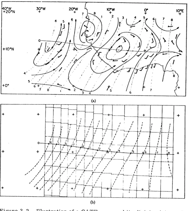
III and the preceding interphase period of GATE (23 August - 19 September). They divided each of these easterly waves into eight north-south bands
(see Figure 3.2). The second band was centered on the region of maximum northerly wind component west of the trough; the fourth, on the trough; the sixth, on the region of maximum southerly wind component east of the trough; and the eighth, on the following ridge. Bands 1, 3, 5, and 7 occu-pied intermediate positions, The, positions were based on the 700-mb flow along the path of the wave disturbance center (defined as the position of the maximum vorticity). Reed et al. referred to these bands as cate-gories or phases, but in this thesis they will be referred to as sectors. The sectors were divided into seven east-west rows, 4* of latitude deep with the center of the disturbance at the midpoint of the middle row. Figure 3.2 shows how this process was accomplished for one of the waves.
Figure 3. 2. Illustration of a GATE wave and its division into sectors. The streamline analysis in (a) was accomplished on fil-tered 700-mb winds. Orientation of the features defining the sectors is shown as slanting, dashed lines. The
sectors are oriented N-S as shown in (b), centered on the points where the defining features cross the path of the disturbance center, the E-W line marked with a zero. (from Reed, et. al., 1977)
The streamline analysis was based on winds which had been band-pass filter-ed to rfilter-educe waves of shorter than two days and longer than six days to less than half-amplitude, while retaining almost fully waves of three to four day period. The east-west line marked with a zero delineates the path of the disturbance center. Each wave was divided into 56 boxes in the manner shown and the observations were averaged in each box to produce the composite wave.
Reed and his colleagues found that the waves propagated westward at an average speed of 8 m se c in the zone of cyclonic shear to the south of the 700-mb easterly jet. The mean latitude of the disturbance paths was 12*N, the mean wavelength was about 2500 km, and the mean period was
about 3.5 days. The maximum low-level convergence and upward vertical motion occurred just ahead of the trough. The maximum cloudiness and pre-cipitation was found just south of the disturbance center in sectors 2 and 3 near the position of maximum convergence and upward motion.
The paths of the centers of the disturbance were at a fairly con-stant latitude. Thus, the B-scale array was usually located in the row of boxes immediately south of the row in which the disturbance paths were centered. Since the waves were usually tilted on NE-SW axes, the wave features generally passed over the array a few hours before the wave sector indicated that they did (e.g. the troughs usually passed over the array a few hours before the array was located at the midpoint of wave sector 4). This effect may be seen in the wave depi.cted in Figure 3.2.
The wave sectors discussed in this section will be referred to in Chapters 4 and 5 in order to describe the general synoptic situations under which the cells being modeled occurred.
3.3 Radar Data
3.3.1 Source
The general approach to the collection of radar data during GATE is described by Hudlow (1975). The radar data used in this thesis were collected with the WR73 radar belonging to the M.IT. Weather Radar Re-search Project. This 5.7-cm radar was located aboard the Gilliss, one of the ships in the B-scale array (see Figure 3.1). The radar generally sampled once every 15 minutes, occasionally less often when significant convection was not present. Each sampling was an elevation step sequence
in which 3600 of azimuth were scanned at a number of elevation angles, This provided three-dimensional data for constant altitude displays, ver-tical cross-sections, etc. Weather echoes were averaged to eliminate frequency fluctuations, range-normalized, and recorded digitally in 512 range bins along each azimuth. The range bins were set up to cover the 256 km range of the radar in such a way as to provide finer range resolu-tion near the radar. This method gave the reflectivity data finer reso-lution where they were more reliable and made the range resoreso-lution more consistent with the vertical and azimuthal resolutions. A complete des-cription of the processed radar data from the Gilliss may be found in Austin (1976).
3.3.2 Handling
Most of the analysis of radar data in this study involved the use of three-dimensional (3-D) radar maps. These maps were constructed from the polar data described in the previous section by superimposing a three-dimensional rectangular box over the area of interest, dividing that box
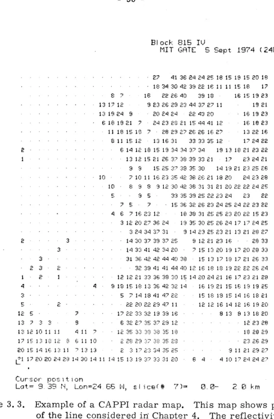
horizontally and vertically into a grid of smaller boxes, and averaging the reflectivity data observed within each small box. The result was a "stack" of constant-altitude plan position indicator (CAPPI) maps, each of which was a horizontal cut through the region at a given level showing equivalent radar reflectivity factor (Z) in dBZ organized on a cartesian plane. Figure 3.3 is an example of a CAPPI radar map, The horizontal resolution of the CAPPI's was 1 km for both the line considered in Chap-ter 4 and the clusChap-ter considered in ChapChap-ter 5. The 3-D radar maps for the line were composed of seven layers, each -2 km deep, so that the maps covered a vertical depth of 14 km. The 3-D maps for.the cluster had a vertical resolution of 1 km and were composed of from seven to ten layers.
Maximum-tops'radar charts were used to compare model cells to observed cells. These "max-tops" charts were generated by determining geometrically the maximum height at which precipitation was detected above each carte-sian grid box. This was accomplished by searching through polar data from progressively higher elevation angles. The max-tops charts for the line had a horizontal resolution of 4 km while the charts for the cluster had a 2-km resolution. The tops in both sets of charts were recorded to the nearest kilometer.
3.3.3 Analysis
[NOTE ON TERMINOLOGY: In this thesis the terms updraft and down-draft, when applied to the model, will refer to the inner and outer cylin-ders, respectively, of the model. When applied to radar data, the term updraft will refer to the intense reflectivity core of a cell wherein active convection is presumed to be taking place and will be understood
Block 815 IV
MIT GATE S Sept 1974 (249)
8 -16 27 18 2.3 20 24 1:3 15 21 15 16 93 13 1712- 3 13 19 24 9 - 6181921 ? 11 18 15 18 ? 8 11 15 12 -614 1218 13 1215 3 3 10 210 11 10 8 3 8 ?25 -2? S 4 6 16 23 - 31220 27 - - 3 32434 -143037 -- 143341 - - - - 31 36 42 - 32 39 - 1212 21:33 4 918151813 - 5 14 18, - 22 20 22 - 1 22 33 32 6 :32 2735 12 3: 5 3332 0 E 28 29 37 13 - 2 :3 17 23 1,4 11 1.415 13?19 3-41 36 2 30 42 3 26 40 29 23 4 24 2 2' 211 23 22 2 31 3 .34 .34 3 37 38 3 37 3 3 35 42 3 30 42 3 33 35 3 15 36 3 18 3 -13 3 91 25 20 40 38 44 40 1 30 15 1 32 14 22 -2 -. 12 13 - 2 3 2 2 3 1- 10 11 3' 12 10 11 112 015 14 16 13 ~1 17 2020 24 '4 )4 2 5 24 2S 22 16 39 18 32 27 43 20 44 41 26 16 .33 35 7 34 19 13 18 9 33 21 1? 5 30 14 13 21 6 26 21 18 20 6 31 31 21 20 22 9 25 22 2324 :2 26 23 24 25 24 8 31 25 25 23:20 5 30 25 26 24 17 4 23 25 23 21 13 912212316 -? 15 13 20 19 12 - 15 13 17 18 17 2 16 18 18 13 22 4 20 24 21 16 17 16 13 21 15 16 - 15 18 1 15 14 12 12 16 14 12 8 13 9 -4311 6 4 -4 10i17
Cursor pos i t ion
Lat= 9. 39 N, Lon=24.66 W, si ice(# 7)= 0.0- 2. i km
Figure 3. 3. Example of a CAPPI radar map. This map shows part of the line considered ini Chapter 4. The reflectivities, given in dBZ for 1X1 km grid points, were determined
by averaging over the layer from 0-2 km. The 3-D map
from which this CAPPI was made extended to a height of 14 km and was composed of seven of these CAPPIs.
47 11 3 16 23 12 35 18 35 25 :31 20 -2 4 11 1 11 7 13 2:8 14 30 1 24 31 34 44 41 38 42
to be analogous to the inner cylinder of the model. The term downdraft, when applied to radar data, will refer to the region surrounding the
active convection wherein compensatory vertical motions are taking place, and will be understood to be analogous to the outer cylinder of the model. These terms will be used to describe regions, not vertical motions, with full awareness of the fact that descent may sometimes occur in the "up-draft" and ascent may sometimes occur in the "downdraft".]
It was necessary during the course of this study to inspect an area or line of convective activity to identify individual cells and de-termine the size of their updrafts. The precipitation in these areas and lines was nearly always spatially continuous. Thus, it was difficult to determine the boundaries between cells. Since the nature of the model requires that each cell be a separate entity, cells and updrafts had to be defined in such a way that individual cells would be separated from each other.
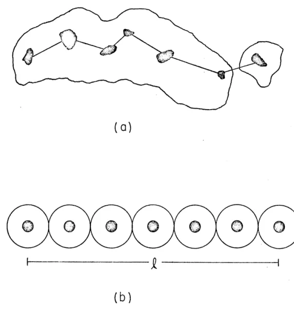
CAPPI radar maps, similar to the example in Figure 3.3, were used to identify cells and determine their updraft areas. If one assumes that a peak reflecticity marks the center of a cell, a reasonable way to deter-mine the extent of its updraft is to search outward from the peak until a sudden, strong decrease, say 3 dB (representing a reduction by half), in the reflectivity is encountered. This point would mark the outer edge of the updraft. Unfortunately, such a sharp reflectivity gradient was often absent from the data, and, when present, often delineated unrealistically large updrafts. In order to avoid these problems, it was necessary to adopt somewhat less logical but more broadly applicable rules for defining
individual cells, it was assumed that the reflectivity between cells must at some point be less than or equal to half the maximum reflectivity. Thus, a reflectivity core was identified as a cell if its point of maxi-mum reflectivity could not be connected to any other cell without crossing a point where the reflectivity was three or more decibels less than its
(own) maximum. This left some flexibility in defining the extent of the updraft. The updraft area could have been defined as the area covered by data points containing the maximum reflectivity. However, the sampling problems inherent in radar observations and in transposing from polar to cartesian coordinates made the use of such a restrictive definition unwise.
Instead, the two remaining possibilities for the definition of an updraft were used. The first definition assumed the updraft area to be that area having reflectivities of the maximum value or one decibel less than the maximum value. The second definition assumed the updraft area to be that area having reflectivities of the maximum value or one or two decibels
less than the maximum value. Both of these definitions are consistent with the rule used to separate the cells in that neither allows the up-drafts of neighboring cells to overlap.
Figure 3.4 shows how the process worked. Two cores, each having a maximum reflectivity of 48 dBZ, have been identified and are shown in-side squares. Note that they cannot be connected without passing through a point where the reflectivity is three or more decibels less than the maxima. The updraft areas based on the first definition are contained within solid lines. In the upper cell part of this area is not contiguous with the reflectivity core. This is probably a result of the noisy nature of the data. Peculiarities of this sort appeared often in the radar data
Block 81 V
MIT GATE 5 Sopt 1974 (248)
12 11 11 15 18 12 10 11 14 18 12 10 9 11 13 8 S 11 11 11 4 2 10 11 11 3 8 12 13 17 8 13 19 21 3 812 18 21 4 11 15 20 4 10 11 13 17 8 14 16 18 1 121517 13 21 522 1 15 116 - 514 - 10 22 23 23 20 2320 16 16 19. 14 12 12 15 18 16 18 13 18 22. 21 21 24 25 28 2R 30 33 26 34 32 22 3~2 35 24 32 32 26 31 33 28 30 33 25 29 33 2 4 33 -- 35-21 36 372 17 31 36 11 ~2 14 13 23 20 9 5 9 11 12 18 19 15 23 2 24 11 22 -13, 2 11 10 11 12 12. 16 24 14 24 23 21 .33 37 33 36 14 31 39 4344 20 32 39 42 44 30 27 34 41 45Z 28 35 3i 42 454 32 38 41 45 (4G 34 4 46 4s' 2.4 3 38 43 44 28- 3? 38.4L 44 31 39 4 32~ 39 44.-A6/45 26A 36 42~ 40* 36 22 30- 38 46 51 16 25 21 40 36 20 17 15 20 26 30 24 12 14 18 27 26 18 22 20E 18 20 22 20 3436 36 25 24 24 2526 25 16 12 21 6 9 11 14 1? 19 21 25 24 35 36 41 40 27 24 24 30 31 18 3 7 - 12 1 18 20 20 24293 3:3547 382624 233:0 2.734 10 13 16 22 29 23 29 .3 41 5 038 28 23 24 27 :30 38 14 12 ?13 26 28 30 26 39 43 4?:330353S03.3132211611 . . .6 27 22 32 28 36 43 45 3 4141 40 42 42 23 25 14 15 -.-26 23 33 34 40 42 43 41 44 46 42 44 39 24 21 19 16 8 27 27 3.3 38 40 40 42 43 44 43 44 40 26 23 24 19 17 - 8 26 2? 3436 40 4246Q48484542 352625C2217? - 8 21141 26 26 283740-41 46 4 4 463235 26 23 18 19 12 12 11 11 14 1 28 31 :30:C 36 40 43 46 47 44 41 32 34 26 24 19 15 15 13 12 15 14 16J 30 32 32 36 45 46 45 4.3 42 30 23 27 24 26 21 16 17 12 18 18 15 16. :31 33 33 35 40 46 41:32 29 26 23 21 27 21 23 21 24 23 23 23 18 19 3- 32 6:3946 44 42 38322621 22 29 21 23 25 26 29 33 2518 211 29 34 39 42 44 4541:39:34 28 2523:30 222427 28 31:3?721 22 201 J33 36 4154244 424140393133 26 25 26 28 25 :31 35 22 2.3 21 36:33404241 404241 3533 393530 29 27 30 2521 22 23 21F 353 39 39 39.33-4 44033 37 41 393G6:33 26 33 28 20 21 22 21E 34 35 33 :36 :38 3? 40 10 42 35 31 41 44 38 32 333328252323V2323 32 34 33 34 36: 33 38 :39 .36 3:3 42 42 45 39 36 30 29:30 23 23 2.3 35333334333433.323332 42 44 42 38 32 2722892822 24 23 38 32 32 34 32 3.3 :31 31 28 32 43 42 4239. 3534:31 2825 2.3 22F 41 36 34:32:3134*33P232 41 41 45 423836 35 30 29 25 23 22 22 42 32 35 :32 29 30 :32 34 36 41 44 41 39 40 40 38 .36 28 25 22 22F 43 32 34 33 32 29 .3335 40 42 40 41 40 41 .38 38 30 30 28 24 24 24 433 3634 35333338404141 41 40 39 331322928 2523 4 42 3 3 34 :30 33 40 :39 .9 43 43 40 38 38 40 38 .33 28 27 26 202 , 3 33 3 36 2233 37 38 45455 4 41 39 41 40 34 31 212422 45 33 36 3 34 30 32 35 3944 4542 42 39 42 40 39 36 .33 28 2621 4.3 38 35 :34 34 34 32 :32 40 43 39 39 43 40 43 :39 :35 34 28 25 222 45 41 32 3932:3938.38 40 35 :38 :38 36 41 42 41 40 38 3:3 332 30 2? 2 4 2 40 33 '39 .36 353:3G3 3335 39 40 39 4236 31 29 28 30 42 34 32232?3"13:36.37.30:3431 2123242 3e.34 30 3230 272 3738363440383634.3133 31 2929 3 :40 4 034222828 25272 46 44 38 39 4.3 42 40 :35 36 .31 30 29 28 36 42 :33 26 26 22 24 25 2.3 43 39 43 42 42 42 41 39 37 32 36 22 40 36 33 25 25 21 22 24 181 37 42 40141 3.941 3238 3933293341 3322 20 21 21 3:345 33938 38 38 36 335 -43 3731 31 2224221415 20 30 37 42 41 41 ? ? 3 34 35 35 3 0 34 27 18 2? 14
-Figure 3. 4. Example of the use of a CAPPI radar map to identify cells and define their updraft areas. See text for explanation. 16 20 19 1.3 9 14 19 18 12 12 19 19 13 13 20 21 2.3 21 20 20 21 2 20 19 21 20 21 1.3 9 2 3 10
and had to be dealt with by objectively applying specific, subjectively-determined rules. The areas based on the second definition are contained within dashed lines. Note that in spite of the fact that the cells have the same maximum reflectivity, their updraft areas (as defined) differ considerably. Since the map has a horizontal resolution of 1 ki, the up-draft areas can be found by simply counting the blocks within the outlined regions.
3.3.4 Idealization
A close inspection of the radar data in Figure 3.4 reveals a sub-stantial variability in cell characteristics. This type of variability was present in all the radar data for the line and the cluster. It is not clear whether it was due to actual differences in cell characteristics or arose from sampling similar cells at different times in their life his-tories. In any case, this variability posed problems both in selecting appropriate input variables for the model and in making comparisons between observed and modeled cells.
In order to determine suitable input variables, the features (i.e, the line and cluster of cells) were idealized into geometrically simple combinations of "representative" cells. The idealized features had the same number of cells as the observed features, but the representative cells in the idealized features were identical with each other and geometrically compatible with the model (i,e. they were composed of an inner cylinder which was the active core or updraft region of the cell, and an outer cylinder which was the "environment" or area where compensating motions >take place. This idealization process is described in section 3.3.4.1.
Since the model would be simulating a "representative" cell, it was also necessary to determine representative values of the characteristics of the observed cells with which to compare model cells. The process for determining representative characteristics for comparison is presented in
section 3.3.4.2.
3.1.4.1 Determination of Input Variables
Although the idealization processes for the cluster and the line were not identical, they had some common features which will be discussed in this section. The features peculiar to the idealization processes for the line and the cluster will be discussed in sections 4.1.2.1 and 5.1.2.1, respectively.
Because it was necessary to build some rather arbitrary definitions into the idealization process, some flexibility was also built into the process. As a result of this flexibility, the idealization process will produce a number of sets of input variables from which a choice of the most realistic values of the variables may be made based on intuitive
judgment, theoretical reasoning, and field observations of these variables. The first step in the idealization process was to determine which cells would be used in the process. The method of identifying cells on a CAPPI radar map was given in section 3.3.3. For the two CAPPI's nearest the ground, the cells were identified and their maximum reflectivity fac-tors were recorded. Cells were then said to "exist" for the purpose of the idealization if they met certain criteria. The criteria varied (this variation provided some of the flexibility built into the process), but in all cases required that an identified cell exist in both of the lower
or both layers. These criteria will be referred to as the E (for exist-ence) criteria. The E will be followed by two subscripts, The first sub-script will prescribe the minimum reflectivity required in one layer and the second will prescribe the minimum reflectivity required in the other layer in order for a cell to be included in the idealization process. For example, E30,1 will refer to the criterion requiring that a cell with
a reflectivity of at least 30 dBZ will exist in one layer and some cell exist in the other layer. Similarly, E40,4 0 will refer to the criterion
requiring that cells with reflectivities of at least 40 dBZ exist in both layers. It was also required that the cells in the two layers exist in reasonable geographical proximity.
The method, described in section 3.3.3, for determining the areas of updrafts involved counting the data points surrounding a core of maxi-mum reflectivity which had reflectivities within a given range of the maximum. The two ranges used in this study form the A (for "area")
cri-teria. A1 will refer to an updraft area determined from data points
having the maximum reflectivity or reflectivities one decibel less than the maximum. Similarly, A2 will refer to an updraft area determined from data points having the maximum reflectivity or reflectivities one or two decibels less than the maximum.
Updraft areas based on both A1 and A2 criteria were determined
from the CAPPI's for the lowest two layers. Although the updraft area in the model is constant with height, the updraft areas determined from the
radar data were seldom the same for both layers, Thus, methods were de-vised to combine the data from the two layers into one area, The two devised methods form the C (for "combination") criteria. Cavg will refer
to the updraft area determined by averaging the areas of the updrafts in the two layers while Cmax will refer to the updraft area determined by using the maximum area of the two layers,
The idealization processes for the line and the cluster employed different E criteria (i.e. the concept was the same but the subscripts were different). Both, however, used the same A and C criteria, The downdraft area of the cells in the cluster were determined by an entirely different process than that used for the cells in the line; these processes will be described in the following chapters.
3.3.4.2 Determination of Cell Characteristics for Comparison of Observed with Model Cells
The model provides fine time- and height-resolution information on such processes and properties as entrainment, vertical velocity, con-densation, water content, forcings, etc. However, little is known about these processes in real situations because they are so difficult to measure. The only property which was available from the model and which was observed
in some useful resolution in the field was radar reflectivity (the model calculates radar reflectivity from the drop size distribution), The radar
data had sufficient spatial resolution to deal with most precipitating
convective elements. Unfortunately, while its time resolution (15 min)
was sufficient for studying mesoscale and synoptic-scale precipitation features, it was too coarse to allow more than a single "snapshot" of a cell taken at a random time in its life. It was possible, if the timing was right, for the same cell to appear on two consecutive radar maps. However, it was rarely possible to identify these as the same cell because of the confusion created by neighboring cells. Therefore, while the model
produced a life history of the reflectivities within themodeled cells, no corresponding life history of observed cells was available. The problem, then, was to devise methods by which fine time- and height-resolution reflectivity data from a single cell simulated by the model could be com-pared to somewhat coarser height-resolution reflectivity data from instan-taneous samples collected by the radar at random times in the lives of a number of cells. To address this problem, three cell characteristics were chosen: the maximum height, the maximum reflectivity, and the height of the maximum reflectivity.
Maximum Height
In vigorous convective situations ice crystals are usually found in the upper portions of the cells, These slowly-falling particles may blow off as an anvil or remain as debris after the intense lower portions of cells have rained out. In any case, they remain aloft for relatively long periods of time, so that when a number of cells occur in the same area, they tend to form a precipitation canopy over the area. The height of the canopy is not as time-dependent as the features of the individual cells and thus serves as a good indicator of the height which the more
vigorous cells attained. Not all cells, of course, reach the height of the canopy, and occasionally very vigorous cells will penetrate it. How-ever, it will be assumed in this study that the height of the canopy cor-responds to the vertical extent of the representative cells. Maximum-tops radar charts were used to determine heights of cells in this study.
Maximum Reflectivity
each observed cell in the lowest two CAPPI's was determined. This allowed the construction of the distribution of maximum reflectivities in the up-drafts of the observed cells. The model output allowed the determination of the distribution with time of the maximum reflectivity in the model cell updraft. These distributions were compared. However, it is important to notice that the comparison was made between the time spectrum of maxi-mum reflectivity for a single modeled cell and the spectrum of
instanta-neous maximum reflectivity for a large number of observed cells, In order for such a comparison to be meaningful, it must be assumed that the ob-served cells were sampled at random times during their lifetimes. Further-more, since the observed cells had varying degrees of representativeness, this comparison must be viewed as a somewhat subjective indication of the model's ability to simulate the observed cells.
Height of Maximum Reflectivity
The approach applied to comparing maximum reflectivities, described in the previous paragraph, was also applied to comparing the height of the maximum reflectivity in the cell updrafts. The model output provided these
heights throughout the life of the cell. For the cluster of cells consi-dered in Chapter 5, the cell population and organization was such that the heights could be determined by manual inspection of the CAPPI's. However, because of the large number of cells and the nature of their relationships with each other, the application of this manual inspection technique was not feasible for the line. Instead, a computer program was written which searched up each column in the 3-D radar charts for the line and recorded the height at which the maximum reflectivity occurred and that maximum
value. The distribution of height versus the number of columns with maxi-mum reflectivities at that height was then found for reflectivities above given thresholds. There were two drawbacks to this automated approach. First, except for the highest thresholds, the distributions probably in-cluded data from some columns which were not actually located in the cell updrafts. Secondly, any tilting of the updrafts which occurred might permit more than one maximum height to be recorded for a single updraft and thus tend to spread the distribution. These drawbacks increased the subjectivity, already alluded to in the previous paragraph, of this com-parison scheme.
3.4 Upper Air Data
3.4.1 Source
The upper air data used in this study is described in Acheson (1976). It was gathered by rawinsonde ascents launched every three hours from the seven ships in the B-scale array. It consisted of temperature,
humidity, wind, and height data every 5 mb.
3.4.2 Handling
Temperature and relative humidity data were to be loaded into the model at 500 m increments from the surface to 15 km. Thus the extremely fine vertical resolution of the data was unnecessary and somewhat of a nuisance. The observed temperature and relative humidity data were con-, verted to a form more consistent with the model requirements by taking centered averages of the data from 250 m below to 250 m aboye the heights at which data would be loaded into the model. These mean temperatures and
relative humidities were then plotted against a linear height scale exten-ding from the surface to 15 km.
3.4.3 Idealization
Although there were no soundings taken in the midst of the line or cluster, there were numerous soundings available from their general vicini-ties. These profiles of temperature and relative humidity, while having major characteristics in common, varied enough over space and time to make difficult the determination of the actual environment in which the convec-tion was taking place. To avoid this difficulty, idealized profiles,
based on a number of soundings, were constructed in such a way as to retain the general characteristics of the actual soundings while ignoring the minor variations. The first step in this idealization process was to
identify the important characteristics -- dry or moist layers, points where gradients changed suddenly, etc. Since all profiles did not have the same characteristics, it was necessary in some cases to identify more than one type of profile. The properties of the major characteristics (thickness, height, maximum or minimum value, etc.) were then averaged to produce in-formation from which an idealized sounding could be constructed for each type of profile. The temporal and spatial distributions of the idealized soundings were then investigated to determine which would provide the most realistic initialization for the model. The specifics of the idealization process are given in the following chapters.