A Computational Study of Flexible Routing
Strategies for the VRP with Stochastic Demands
by
Kirby Ledvina
S.B. Economics
S.B. Management Science
Massachusetts Institute of Technology, 2017
Submitted to the Department of Civil and Environmental Engineering
in partial fulfillment of the requirements for the degree of
Master of Science in Civil and Environmental Engineering
at the
MASSACHUSETTS INSTITUTE OF TECHNOLOGY
February 2021
© Massachusetts Institute of Technology 2021. All rights reserved.
Author . . . .
Department of Civil and Environmental Engineering
January 12, 2021
Certified by. . . .
David Simchi-Levi
Professor of Civil and Environmental Engineering
Thesis Supervisor
Accepted by . . . .
Colette L. Heald
Professor of Civil and Environmental Engineering
Chair, Graduate Program Committee
A Computational Study of Flexible Routing Strategies for the
VRP with Stochastic Demands
by
Kirby Ledvina
Submitted to the Department of Civil and Environmental Engineering on January 12, 2021, in partial fulfillment of the
requirements for the degree of
Master of Science in Civil and Environmental Engineering
Abstract
We develop and numerically test a new strategy for the vehicle routing problem with stochastic customer demands. In our proposed approach, drivers are assigned to predetermined delivery routes in which adjacent routes share some customers. This overlapping assignment structure, which is inspired by the open chain design from the field of manufacturing process flexibility, enables drivers to adapt to variable cus-tomer demands while still maintaining largely consistent routes. Through an extensive computational study and scenario analysis, we show that relative to a system without customer sharing, such flexible routing strategies partly mitigate the transportation costs of filling unexpected customer demands, and the relative savings grow with the number of customers in the network. We also find that much of the cost savings is gained with just the first customer that is shared between adjacent routes. Thus, the overlapped routing model forms the basis for a practical and efficient strategy to manage costs from demand uncertainty.
Thesis Supervisor: David Simchi-Levi
Acknowledgments
I would foremost like to thank my advisor David for welcoming me into his research group and entrusting me with a new idea to integrate process flexibility and trans-portation. I am also deeply grateful to Dr. Yehua Wei and Hanzhang Qin, who were crucial collaborators in developing this new research direction. Thank you also to Blue Yonder for its early sponsorship of our work. Finally, I will forever appreciate the consistent encouragement, patience, and support I have received from my family and my friends within the MIT community.
Contents
1 Introduction 11
2 Related Literature 15
2.1 VRP with Stochastic Demands (VRPSD) . . . 15
2.2 Process Flexibility . . . 18
2.3 Collaborative Routing . . . 20
3 Flexible Vehicle Routing 23 3.1 Model Setup . . . 23 3.1.1 Notation . . . 24 3.1.2 Recourse Policies . . . 26 3.2 Example Problem . . . 28 3.3 Asympototic Performance . . . 36 4 Computational Study 37 4.1 Simulation Setup . . . 37 4.2 Baseline Results . . . 38 4.3 Scenario Analysis . . . 44 5 Conclusion 53 A Simulation Code 59 A.1 Main Function . . . 59
List of Figures
1.1 Types of operational flexibility . . . 12
2.1 Network structures in manufacturing process flexibility . . . 19
2.2 Example of marginal gains from increasing flexibility . . . 19
3.1 Route assignments for a network with three vehicles . . . 26
3.2 Giant tour, primary routes, and extended routes in the example problem 29 3.3 Primary routes and realized trips under dedicated routing in the ex-ample problem . . . 31
3.4 Extended routes and realized trips under overlapped routing in the example problem . . . 32
3.5 Vehicle-customer assignment networks in the example problem . . . . 33
3.6 Realized trips under full flexibility in the example problem . . . 34
3.7 Reoptimized routes once demands are known in the example problem 35 4.1 Average cost in the baseline scenario . . . 40
4.2 Histogram of routing costs in the baseline scenario . . . 41
4.3 Average circular and radial costs in the baseline scenario . . . 42
4.4 Average number of trips in the baseline scenario . . . 44
4.5 Circular and radial costs by routing strategy in the long route, short route, and baseline scenarios . . . 48
4.6 Percent of instances in which the cost of overlapped routing is equal to, higher than, or lower than the cost of dedicated routing in the binomial demand, stochastic customer, and baseline scenarios . . . 51
List of Tables
3.1 Realized customer demands in the example problem . . . 30
3.2 Summary of dedicated routing in the example problem . . . 30
3.3 Summary of overlapped routing in the example problem . . . 32
3.4 Summary of full flexibility in the example problem . . . 34
3.5 Comparison of all routing strategies in the example problem . . . 35
4.1 Average cost in the baseline scenario . . . 39
4.2 Percent of instances in which overlapped routing yields higher cost, equal cost, or lower cost compared to dedicated routing in the baseline scenario . . . 42
4.3 Average radial share of total cost in the baseline scenario . . . 43
4.4 Average number of trips in the baseline scenario . . . 43
4.5 List of scenarios . . . 45
4.6 Average cost of overlapped routing relative to dedicated routing in the small overlap, medium overlap, and baseline scenarios . . . 46
4.7 Average cost in the high capacity and low capacity scenarios relative to the baseline scenario . . . 47
4.8 Average number of trips in the long route, short route, and baseline scenarios . . . 49
4.9 Average cost in the binomial demand, stochastic customer, and baseline scenarios . . . 50
4.10 Average total and relative costs of overlapped routing in the baseline, binomial demand, and stochastic customer scenarios . . . 51
Chapter 1
Introduction
Organizations operate amidst several economic, political, and environmental uncer-tainties. Thus, decision-makers in these organizations often adopt risk management strategies to navigate uncertainty when planning day-to-day operations and develop-ing longer-term strategies. In the context of operations, one strategy to enable efficient responses to uncertainty is to incorporate flexibility, which Simchi-Levi (2010) defines as the ability to respond to change at minimal cost.
Flexibility in practice looks different across organizations and functions. Figure 1 illustrates three forms of operational flexibility in the context of manufacturing: system, process, and product design flexibility (Simchi-Levi 2010). System flexibil-ity is achieved through coordinated manufacturing and distribution networks. For example, manufacturers can enable their factories to build multiple product types; then if there is unforeseen demand or a disruption in manufacturing for a particu-lar product, production capacity elsewhere in the network can be utilized. Process flexibility refers to adaptable operations within individual product lines and network locations. For example, worker cross-training ensures workers have the skills to per-form multiple tasks and fill staffing gaps as needed. Finally, product design flexibility ensures that new products are developed with responsive supply chains. For example, a modular product structure facilitates last-minute customization in response to con-sumer demands. The modular structure also allows for individual product parts to be reused or replaced. In all of these examples, organizations designed and installed
flexible systems and procedures in advance to make their operations more responsive to change.
Figure 1.1: Types of operational flexibility
For this thesis, we propose a strategy for incorporating flexibility into transporta-tion and last mile distributransporta-tion. We explore a setting in which a transportatransporta-tion services provider (distributor) operates a vehicle fleet that makes daily deliveries of a single product type to retail customers. Each day, the distributor executes a priori delivery routes designed in advance around expected order quantities, vehicle capacity, and various logistical constraints. The consistency of these fixed routes allows the dis-tributor to enter longer term and lower cost contracts with carrier companies (fleet owners), support driver familiarity with the route, and promote positive customer relationships (Bertsimas 1992, Erera et al. 2009). However, customers may unexpect-edly update their orders, and it can be costly for the distributor to accommodate these changes. For example, the distributor may face procurement costs from ac-quiring last-minute vehicles and drivers for additional deliveries. There may also be customer service costs if drivers change from day to day or if some orders cannot be filled. Additionally, while the existing literature in operations research provides reop-timization approaches to update delivery routes based on new customer information, reassembling routes may not be logistically feasible in a short planning window.
In the setting we consider, if the actual quantities demanded by a route’s cus-tomers exceed the vehicle’s capacity, then the vehicle experiences a route failure, and the driver must return to the product depot to restock, increasing transportation costs. Performing a refill trip as described here is an example of a recourse policy,
which describes how drivers should respond upon experiencing a route failure. Typi-cally, under what we call a dedicated routing strategy, routes consist of exclusive sets of customer so that each driver is individually responsible for its assigned customers’ orders. However, transportation costs from necessary refill trips grow quickly with the number of customers. Therefore, we explore an alternative, flexible strategy called
overlapped routing that mitigates the costs accrued through route failures. Under
overlapped routing, the a priori routes are designed with overlap such that neighbor-ing routes share some customers. Then, with coordination from the distributor or other central planner, drivers visit a narrowed down subset of customers within their predesigned routes in response to realized customer demands. This overlapping de-sign, inspired by the existing literature in manufacturing process flexibility, maintains much of the route consistency of the dedicated routing strategy while allowing the distributor some flexibility to adjust to changing demands.
In their working paper, Ledvina et al. (2020) first proposed the overlapped rout-ing strategy and provided a theoretical guarantee on its cost in problems with a infinitely large number of customers. The researchers also explored the strategy’s non-asymptotic performance through a computational study. Here, we expand on their work with additional scenarios and analysis made possible through revamped simulation code. Through this work, we find that when vehicle capacity is an active constraint, trips to and from the depot drive increasing transportation costs as the number of customers grows. However, overlapped routing harnesses surplus capacity within the vehicle fleet to mitigate these costs. More specifically, through customer sharing, vehicles with excess capacity can assist with deliveries along a neighboring route and sometimes prevent the need for a refill trip elsewhere in the network.
The next chapter provides an overview of the related literature in vehicle routing and process flexibility. Chapter 3 formally defines the routing models and walks through the proposed recourse policies. Chapter 4 describes the computational study on the cost-saving potential of flexible vehicle routing and provides simulation outputs and findings. Chapter 5 concludes.
Chapter 2
Related Literature
In this chapter we review the research that motivates or overlaps with our proposed flexible routing strategy and customer sharing scheme. First, we identify our position within the vehicle routing problem (VRP) with stochastic customer demands. Then we introduce key concepts from the literature on manufacturing process flexibility, which inspires the design for our model’s fixed, yet flexible, routes. Finally, we touch on the field of collaborative vehicle routing – a subarea of freight logistics – which explores customer sharing in mostly non-stochastic settings.
2.1
VRP with Stochastic Demands (VRPSD)
The VRP with stochastic demands (VRPSD) describes a class of routing problems in which customer demands are uncertain (Dror et al. 1989, Gendreau et al. 2014). In contrast, the deterministic VRP addresses settings in which customer demands – as well as travel times, costs, and other possible sources of randomness – are fixed and known. Typically, the objective in the VRPSD is to design vehicle routes that minimize the cost of filling the unknown demands subject to a set of unique, setting-specific constraints, e.g., related to fleet size, vehicle capacity, service level targets, delivery time windows, etc. However, solution methodologies depend on each prob-lem’s specific characteristics as well as any assumptions on the likely distribution of customer demands.
Gendreau et al. (2016) review notable models and methods for the VRPSD and separate the problem into the a priori paradigm and the reoptimization paradigm. In the a priori model, routes are fixed in advance before customer demands are realized. Under reoptimization, on the other hand, routes are updated gradually as new de-mand information becomes available. In some cases these updates occur dynamically while the vehicle executes its route. Note that if demands are learned sufficiently early, organizations may have the information, time, and resources to fully optimize their routes, at which point the VRPSD can be solved as a deterministic VRP.
Our proposed flexible routing model uses a priori routing, or fixed routing. In this setting, a route failure occurs if the vehicle exhausts its capacity prior to completing its assigned deliveries. Recourse policies describe how a driver should respond upon experiencing a route failure. Under a classical recourse policy, for instance, the pre-scribed response is that the vehicle must detour to the depot to replenish its inventory before proceeding with its route at the point of failure (Gendreau et al. 2016). This response increases travel costs but is necessary if the driver needs to fully serve its route. Therefore, an important research area is in developing initial routes – or for some approaches, larger tours and customer sequences that can then be split into routes – that yield the minimum travel cost in expectation over variable customer demands.
With a priori routing, typically drivers learn the specific customer demands only upon arriving at the customer location – see, e.g., Secomandi and Margot (2009) and Gendreau et al. (2014). In contrast, our routing strategy assumes that drivers learn customer demands before executing their routes. Other researchers such as Bartholdi III et al. (1983), Bertsimas (1992), and Jaillet (1988) have adopted this as-sumption as well. Bertsimas (1992), for example, evaluates a routing strategy for the VRPSD in which drivers can bypass customers with zero demand and thus decrease transportation costs. Receiving demand information in advance allows for upfront adjustments to the routes that drivers execute. In this way, planners can incorporate some of the flexibility of reoptimization while still preserving some consistency in the initial routes.
Another feature of our proposed flexible routing strategy is overlapped routes, in which delivery vehicles serving adjacent areas share customers. To our knowledge, within the VRPSD literature, only a few other papers consider some version of fixed routing with customer sharing. Erera et al. (2009), for example, propose a fixed routing system and route construction method to accommodate a variable customer list with delivery time windows. In their approach, customers are assigned to both primary and backup routes. Planners then have the option to bump customers from one route to the other to maintain overall feasibility or to lower transportation costs without re-solving the routing problem from scratch.
Ak and Erera (2007) propose a paired vehicle strategy in which vehicles are as-signed a priori routes, matched together in exclusive pairs, and then asas-signed a Type I or Type II designation within their pairs. If a Type I vehicle experiences a route failure, it terminates its route, and the Type II vehicle extends its own route to serve the remaining customers from the Type I route, detouring to the depot to refill as needed.
Lei et al. (2012) also consider a recourse policy with exclusively paired vehicles. In their setup, paired routes can split demands at a single shared customer. The authors derive expected costs of a non-cooperative case in which vehicles fill an optimally predetermined percentage of the shared customer’s demand. The authors also discuss a cooperative case in which a vehicle fills as much demand as possible in certain situations to reduce the chance of the other vehicle’s experiencing a route failure and performing a costly refill trip.
Finally, the working paper from Ledvina et al. (2020) introduces a route chaining design in which non-exclusive pairs of neighboring routes share customers. The chain-ing design is inspired by the literature on manufacturchain-ing process flexibility, further discussed below. Ledvina et al. (2020) derive theoretical guarantees on the asymptotic performance of their strategy, i.e., as the number of customers approaches infinity. Additionally, like Ak and Erera (2007), Erera et al. (2009), and Lei et al. (2012), they present computational results for smaller problems. This thesis builds on Ledvina et al. (2020) with an expanded computational study and sensitivity analysis on the
non-asymptotic costs of the proposed flexible routing strategy.
2.2
Process Flexibility
We employ a fixed route design inspired by manufacturing process flexibility. Jordan and Graves (1995) produced the seminal paper on the principles and benefits of manufacturing process flexibility, which they define as the ability "to build different types of products in the same plant or production facility at the same time" (Jordan
and Graves 1995).1 Factories are assigned to manufacture specific product types
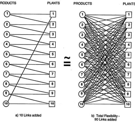
within an overall production capacity. However, demands for each product type are variable, and the system’s flexibility to meet unexpected spikes in demand increases when more than one plant can produce the requested product type. By simulating random demands for different product types, Jordan and Graves (1995) show that a factory-product assignment structure called the long chain achieves comparable service levels (measured as the share of product demand that can be met) as a fully flexible network but with much less investment in redundant production capability. In a fully flexible network, every factory can produce every product. Under the long chain, however, each factory can produce only two product types such that the structure of the factory-product assignment bipartite graph forms a closed chain throughout the network. Figure 2.1 from Jordan and Graves (1995) illustrates this finding on the long chain’s performance.
Simchi-Levi and Wei (2012) later proved that in adding flexibility to an inflexible, dedicated manufacturing system (in which each factory can produce only one product type), the marginal gains in expected service level increase with each additional flex-ible edge, or redundant factory-product assignment. The final link which transforms an open chain graph into a closed, long chain graph yields the greatest incremental benefit of all. Figure 2.2 from Simchi-Levi and Wei (2012) illustrates the process and marginal gains of incrementally adding flexibility to a manufacturing system. In this 1In the literature, "process flexibility" is often used in place of "system flexibility" as defined by Simchi-Levi (2010). Therefore, we will follow Jordan and Graves (1995) in using the term process flexibility to refer to manufacturing networks with coordinated production capabilities.
Figure 2.1: Network structures in manufacturing process flexibility. The long chain assignment structure (a) achieves comparable service levels as a fully flexible network (b). Figure from Jordan and Graves (1995).
example, adding edges (1,2),...,(5,6) forms an open chain network while adding edge (6,1) creates the long chain network.
Figure 2.2: Example of the marginal gains in performance (expected sales) as a manu-facturing assignment network adds flexible edges one-by-one. Figure from Simchi-Levi and Wei (2012).
Ledvina et al. (2020) embedded process flexibility into the VRPSD by adapting the open chain design from manufacturing process flexibility. They find that an open chain structure for assigning vehicles to customers yields considerable savings in transportation costs relative to a dedicated system. Additionally, in their model, these savings grow as the number of customers increases (Ledvina et al. 2020).
Lyu et al. (2019), Asadpour et al. (2020), and Xu et al. (2020) also add process flexibility into delivery applications but consider different settings and performance metrics than do Ledvina et al. (2020). Specifically, Lyu et al. (2019) presents a case study on assigning workers to parcel delivery zones with a long chain structure such that workers serve overlapping zones and can share any high delivery burden. Asad-pour et al. (2020) apply the long chain flexibility design to an online order-fulfillment system with multiple warehouse locations and limited resource inventories. Finally, Xu et al. (2020) extend Asadpour et al. (2020) by considering unbalanced systems with different numbers of warehouses versus product types. These three papers all measure network performance in terms of service level for customer demands while our work focuses on the routing cost of filling all demands. Additionally, Asadpour et al. (2020) and Xu et al. (2020) limit warehouse inventories while our model assumes sufficient inventory to fill all demand.
2.3
Collaborative Routing
Finally, we touch on the literature in collaborative routing in freight logistics. Gansterer and Hartl (2018) define collaborative vehicle routing as “all kinds of cooperations which are intended to increase the efficiency of vehicle fleet operations.” Carriers, distributors, or other logistics service providers may share vehicles, facilities, cus-tomers, or other resources to decrease costs, increase service level, or even decrease emissions among other objectives (Cleophas et al. 2019, Gansterer and Hartl 2018).
Generally, research in collaborative routing focuses on multi-agent environments. Typically, in non-collaborative settings, individual organizations maintain their own information with an eye towards maximizing their individual profits. In contrast, in
collaboration with decentralized planning, participants agree on mechanisms such as auctions or hierarchical decision-making to exchange limited information for collabo-ration. Even more, with centralized planning, all participant information needed for collaboration is known, and the objective is to maximize the joint utility (e.g., profit) of all collaborators. See Gansterer and Hartl (2018) for an overview of the recent literature on models and methods for centralized collaborative planning specifically.
As in the VRPSD literature, a major area of research in collaborative routing is in optimizing vehicle routes and customer assignments, with additional insights into the impact of collaboration size, benefits relative to non-cooperative scenarios, and the design of compensation schemes – see e.g., Sanchez et al. (2016), Quintero-Araujo et al. (2016), Defryn et al. (2016), and Guajardo and Rönnqvist (2016). For exam-ple, Fernández et al. (2018) introduce the Shared Customer Collaboration Vehicle Routing Problem (SCC-VRP) in which customer orders can be transferred among a predetermined set of carrier companies. Each carrier operates its own fleet of delivery vehicles, and the demand filled by any vehicle cannot exceed the vehicle’s capacity. The objective of the SCC-VRP is to minimize the total routing cost across carriers. From their computational studies, Fernández et al. (2018) observe that collaboration yields the most savings relative to a non-collaborative scenario when a larger number of customers are shared over a greater region. Similarly, Sanchez et al. (2016) explore gains from the collaboration of different subsets of carriers and find that the most gains occur with a complete pooling of resources. In their literature survey, Gansterer and Hartl (2018) also observe that the best savings are achieved with complete coop-eration.
Our work in flexible vehicle routing is similar to collaborative routing in that we are also designing routes with customer sharing and quantifying the resulting benefits. However, much of the collaborative routing literature assumes deterministic customer demands or order requests (as well as a multi-agent setting), which allows participants to redesign their collaborations for each realized instance. Quintero-Araujo et al. (2016) produced one of the few collaborative routing studies that does consider stochastic demands. In their model, delivery vehicles are penalized for route
failures; then the overall transportation cost for a set of routes is calculated as the sum of the deterministic VRP cost and the average route failure cost. Still, our flexible routing strategy is most grounded in VRPSD methodologies. Looking now to the next chapter, we will finally describe our proposed strategy in detail.
Chapter 3
Flexible Vehicle Routing
In this chapter, we establish model notation, define two types of vehicles routes, and introduce the dedicated and overlapped recourse policies. Recall that a recourse policy is a planned response to a route failure, i.e., actions to take when a vehicle exhausts its capacity prior to completing its route. For this reason, we often refer to recourse policies as routing strategies. Of the dedicated and overlapped routing strategies, overlapped routing is our proposed flexible approach for settings with a priori routes and stochastic customer demands. For comparison purposes, we also define a fully flexible policy, in which vehicles follow a fixed route but are not restricted to specific customer subsets, as well as reoptimization as alternative routing strategies.
After describing the model, we walk through a concrete example of the routing strategies in a small-scale problem with six customers. Finally, though this thesis focuses on computational results in the non-asymptotic case, we share some key find-ings from Ledvina et al. (2020) on the performance of the overlapped routing strategy as the number of customers approaches infinity.
3.1
Model Setup
Below we formally define the routing models. We establish the relevant notation and describe the routing strategies that we evaluate.
3.1.1
Notation
A fleet of 𝑀 homogeneous delivery vehicles must fill the stochastic daily demands of a set of 𝑁 customers. Vehicles each have a capacity of 𝑄 units, meaning a vehicle can serve 𝑄 units of customer demand before the vehicle exhausts its capacity and must detour to the depot to reload. We assume a single product type. For computational convenience, we also assume the number of customers 𝑁 is divisible by fleet size 𝑀. This way, we can assign vehicles to routes of equal length in terms of the number of customers they may need to visit.
Next we represent customer locations and demands. Customer 𝑖 is located at
position xi ∈ R2 on a bounded plane for 1 ≤ 𝑖 ≤ 𝑁. Delivery vehicles depart from
a single depot located at x0 ∈ R2. Each customer 𝑖 is then the Euclidean distance
c0i = ‖x0−xi‖2from the depot and distance cji = ‖xj−xi‖2 from any other customer
𝑗. We calculate transportation cost as the sum of all costs c0i and cji accrued on the
realized (executed) route. All customer demands are independently and identically
distributed such that customer 𝑖 exhibits random demand 𝐷𝑖 ∼ 𝐷 where 𝐷 covers
some subset of non-negative integers 0, 1, 2, ..., 𝑑𝑚𝑎𝑥. Customer 𝑖’s realized demand for a given day is denoted 𝑑𝑖, and we denote the set of all realized customers demands as 𝒟 = {𝑑1, ..., 𝑑𝑁}.
Vehicles are assigned to a priori routes with a subset of customers according to some predetermined flexibility design. In our model, flexibility refers to the extent of route overlap (customer sharing) between adjacent vehicle routes. Specifically, we identify two types of a priori routes: primary routes and extended routes. Primary routes are defined as disjoint routes with no customer sharing such that each vehicle
𝑚 = 1, .., 𝑀 has an a priori route with 𝑁′ = 𝑁/𝑀 customers. More formally,
define 𝜋 as a tour through all 𝑁 customer locations beginning and ending at the depot, and assign labels 𝑖 = 1, 2, ..., 𝑁 sequentially to the customers in the tour 𝜋.
Then, the primary route for vehicle 𝑚 = 1, ..., 𝑀 is the customer sequence 𝒫𝑚 =
[(𝑚 − 1)𝑁′ + 1, (𝑚 − 1)𝑁′ + 2, ..., 𝑚𝑁′]. To illustrate, this setup means vehicle 1’s
customer sequence [𝑁′ + 1, ..., 2𝑁′], and so on, until we reach vehicle 𝑀’s route 𝒫𝑀 = [𝑁 − 𝑁′+ 1, ..., 𝑁 ].
Extended routes, on the other hand, are designed with some overlap such that adjacent routes share 𝑘 customers. Define the extended route for vehicle 𝑚 as the
customer sequence ℰ𝑚 = [(𝑚 − 1)𝑁′ + 1, (𝑚 − 1)𝑁′ + 2, ..., 𝑚𝑁′ + 𝑘] for vehicles
𝑚 = 1, ..., 𝑀 − 1. The extended route for vehicle 𝑚 = 𝑀 is just ℰ𝑀 = [(𝑀 −
1)𝑁′ + 1, (𝑀 − 1)𝑁′ + 2, ..., 𝑀 𝑁′]. Put differently, the extended route for vehicle
𝑚 = 1, ..., 𝑀 − 1is vehicle 𝑚’s primary routes plus the first 𝑘 customers from vehicle
𝑚+1’s primary route while vehicle 𝑚 = 𝑀’s extended route is identical to its primary
route. Drivers must visit the customers with non-zero demand sequentially within these routes.
Figure 3.1 shows bipartite graphs with vehicle-customer assignments for (i) pri-mary routes, (ii) extended routes with one shared customer (𝑘 = 1), and (iii) extended
routes with overlap size equal to the full primary route size (𝑘 = 𝑁′). Note that these
route assignments parallel the flexibility networks from the manufacturing process flexibility literature. Specifically, the primary routes follow a dedicated network de-sign, and the extended routes resemble the open chain design.
Figure 3.1: Route assignments for a network with 𝑀 = 3 vehicles. Bold lines indicate vehicle assignments to the 𝑘 shared customers for the extended routes.
3.1.2
Recourse Policies
Below we describe the recourse policies for dedicated routing and overlapped routing. We also describe the full flexibility strategy and a separate reoptimization strategy for comparison purposes. All strategies except reoptimization are examples of fixed rout-ing strategies. However, they involve different a priori routes and prescribe different responses to a route failure.
In dedicated routing, vehicles are assigned to their primary routes with disjoint customers subsets. Each day vehicles first receive information on their assigned cus-tomers’ realized demands and identify which specific customers require deliveries. Each vehicle then departs the depot at full capacity 𝑄 and sequentially visits the customers in its primary route 𝒫𝑚, bypassing the customers that have zero demand. If the vehicle exhausts its capacity, the driver detours to the depot to refill to full capacity and resumes its route wherever it left off. Upon filling all customer demands in its primary route, the vehicle has completed its route for the day and returns to the depot.
Under the overlapped routing strategy, vehicles instead are assigned to their
ex-tended routes, which include the 𝑁′ customers in a vehicle’s primary route plus some
𝑘 additional customers (for vehicles 𝑚 < 𝑀). As in the dedicated strategy, each
day vehicles first receive information on realized customers demands. Upon learning demands, vehicles depart from the depot at full capacity and sequentially visits cus-tomers in their primary routes, bypassing cuscus-tomers with zero unfilled demand. Each vehicle 𝑚 detours to the depot to reload as necessary to serve all unfilled demand in primary route 𝒫𝑚. Upon filling demand of the final primary route customer, if all
𝑄 units of capacity are exhausted, the vehicle returns to the depot and concludes its
route. However, if vehicle 𝑚 has any remaining capacity, it sequentially visits and
serves any additional customers in its extended route ℰ𝑚 until the vehicle’s surplus
capacity is exhausted. At this point, vehicle 𝑚 returns to the depot for the day. Then
vehicle 𝑚 + 1 begins its primary route 𝒫𝑚+1 wherever vehicle 𝑚 ended its service.
In the case that vehicle 𝑚 for some 𝑚 = 1, ..., 𝑀 − 1 satisfies the demand of all customers in vehicle 𝑚 + 1’s primary route, then vehicle 𝑚 + 1 does not need to be deployed. We assume that a central planner assesses the realized customer demands and coordinates each vehicle’s starting and ending customers (realized routes) within the extended routes prior to the vehicles’ departing the depot. This way, vehicles can execute their routes simultaneously.
While we focus on overlapped routing as our proposed flexible policy, we can also define a strategy with full flexibility in which any vehicle can serve any cus-tomer as long as the drivers followed the predetermined cuscus-tomer sequence 𝜋. This vehicle-customer assignment structure is inspired by the full flexibility design from the manufacturing process flexibility literature. In executing this strategy, vehicle 1 serves the first 𝑄 units of demand at which point vehicle 1 experiences a route failure. Vehicle 2 continues where vehicle 1 ended and serves an additional 𝑄 units of demand, and so on, until all customers have been served. Depending on the magnitude of total customer demand, the final vehicle 𝑀 may need to make multiple trips to serve all remaining customers. Alternatively, the final vehicles may not be needed at all on a given day if the previous vehicles were able to fill all demand. This strategy closely
aligns with the classical recourse policy analyzed by Bertsimas (1992) and others. The main difference is that our full flexibility model includes multiple vehicles – though it can be simplified to the single vehicle case – which in practice allows for a divided workload with concurrent route execution under the guidance of a central planner.
Finally, reoptimization generates the lowest-cost vehicle routes for each new set of demands. Unlike the fixed route strategies above, reoptimization does not constrain which vehicles can visit which customers or in which order. In the most general case, reoptimization in our setting is solved as a VRPSD with splittable demands in which a customer can be served through multiple visits.
To help elucidate the policies above, we developed a companion Jupyter notebook file in which users can generate random customer and demand instances and see the resulting routes and costs under the different strategies – please refer to Appendix A for more information. We also used this tool to create the example presented below.
3.2
Example Problem
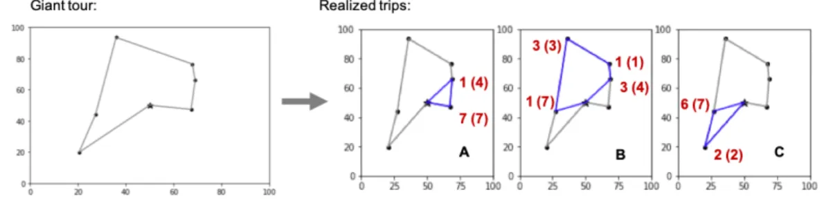
To illustrate the routing models and recourse policies, consider an example with six customers. Each customer has demand randomly selected from 0, 1,..., 8. We have three vehicles in our fleet, so we decide to create three primary routes with two customers each. Each vehicle’s capacity 𝑄 is 8, which is the expected combined demand of two customers on a primary route.
To generate the a priori routes, let’s first create a giant traveling salesman tour through all customers. Select an arbitrary first customer, and label the tour’s cus-tomers sequentially as 1, 2,..., and 6. For the primary routes, divide the tour into three sub-sequences of size 2. Define primary route A with customers {1, 2}, primary route B with customers {3, 4}, and primary route C with customers {5, 6}. For the extended routes, let overlap size 𝑘 be 1, and define extended routes A, B, and C to have customers {1, 2, 3}, {3, 4, 5}, and {5, 6}, respectively. Under this design, adja-cent extended routes A and B share one customer (customer 3) and adjaadja-cent extended routes B and C share one customer (customer 5). Figure 3.2 shows the giant tour, set
of primary routes, and set of extended routes as arranged through customer locations in a Cartesian plane.
Figure 3.2: Giant tour (grey) and resulting primary and extended routes (orange) in the example problem. Customers were randomly placed on a 100x100 grid. The single centrally located depot is marked with a star.
After creating our routes, we learn customers’ actual demands, which may change from day to day. Table 3.1 presents one particular day’s demand for each customer in our example. We will illustrate the dedicated routing, overlapped routing, and reoptimization strategies on this demand instance.
Cust. 1 Cust. 2 Cust. 3 Cust. 4 Cust. 5 Cust. 6 Total
Demand 7 4 1 3 7 2 24
Table 3.1: Realized customer demands in the example problem Dedicated Routing
Recall that in the dedicated routing strategy, each vehicle is independently responsible for its primary route, either A, B, or C. Figure 3.3 shows how each vehicle navigates its primary route to fill its customers’ demands. Here, Vehicle A must fill a total of 11 units of demand on its route, which exceeds the vehicle’s capacity of 8. Because Vehicle A exhausts its capacity while serving Customer 2, the driver detours to the depot to restock before completing its delivery. Vehicle B, on the other hand, faces only 4 units of demand and can serve its customers in one trip. Finally, Vehicle C must fill 9 units of demand on its route, and like Vehicle A, requires two trips from the depot to serve fully serve the final two customers. Table 3.2 summarizes each vehicle’s realized trip count, customers served, and demand filled. Ultimately, this dedicated routing strategy costs 400.1 units, measured as the Euclidean travel distance in filling all customer demands.
Vehicle Number of Trips Customers Served Demand Filled
A 2 {1, 2} 11
B 1 {3, 4} 4
C 2 {5, 6} 9
Total 5 All 24
Routing Cost: 400.1
Figure 3.3: Primary routes and realized trips under dedicated routing in the example problem. Red labels state the demand filled (total demand) at each customer. Overlapped Routing
We now walk through an overlapped routing strategy in which adjacent routes share one customer. Figure 3.4 illustrates the a priori extended routes as well as the real-ized trips for each vehicle under this strategy. In calculating workloads, we iterate sequentially through routes A, B, and C; note, however, that drivers are informed of their updated workloads prior to departure and thus can simultaneously execute their routes.
Vehicle A first executes its primary route as in the dedicated routing strategy. Upon serving Customer 2 in its second trip, the vehicle has 7 units of surplus capacity and thus proceeds to fully serve the 1 unit of demand at Customer 3, the shared customer in Vehicle A’s extended route. Upon completing its extended route, Vehicle A returns to the depot. Vehicle B then begins with the first unserved customer in its primary route, which is Customer 4. Upon completing its primary route, Vehicle
Figure 3.4: Extended routes and realized trips under overlapped routing in the example problem. Red labels state the demand filled (total demand) at each customer. B has 5 units of surplus demand, which it uses to partly serve Customer 5 in its extended route before returning to the depot. Finally, Vehicle C fills the remaining demand at Customer 5 and all demand at Customer 6.
This strategy eliminates the need for the second trip that Vehicle C performed under dedicated routing. Ultimately, as summarized in Table 3.3, the overlapped strategy costs 338.4, a 15% savings over dedicated routing.
Vehicle Number of Trips Customers Served Demand Filled
A 2 {1, 2, 3} 12
B 1 {4, 5} 8
C 1 {5, 6} 4
Total 4 All 24
Routing Cost: 338.4
Full Flexibility
In routing with full flexibility, any vehicle can serve any customer. As illustrated in Figure 3.5, the structure of the corresponding fully flexible assignment network differs from that of dedicated and overlapped routing, in which customers are restricted to certain customer subsets. However, the construction of realized vehicles routes must still follow the customer sequence defined by our giant tour.
Figure 3.5: Vehicle-customer assignment networks for dedicated, overlapped, and fully flexible routing in the example problem. Bold lines indicate assignments to shared customers.
To determine the realized routes, we assign Vehicle A to first serve as much demand as possible. It fully serves Customer 1 but only partly serves Customer 2, at which point Vehicle A experiences a route failure and returns to the depot. Vehicle B then completes the delivery at Customer 2 and manages to fully serve Customers 3 and 4 and partly serve Customer 5 before the vehicle exhausts its capacity. Finally, Vehicle C visits both Customer 5 and Customer 6. As in overlapped routing, this algorithm is used simply to determine the day’s routes; upon initial coordination, drivers can then execute their finalized routes simultaneously.
Figure 3.6 illustrates the realized vehicle routes. The key difference from the overlapped routing solution is that Vehicle B is able to serve Customer 2 which is outside of Vehicle B’s extended route. This ability is especially valuable since it saves Vehicle A a refill trip and, in this example, has no repercussions further along in
the customer sequence. Table 3.4 summarizes realized routes and costs under full flexibility. The total cost of 297.0 is a 12% savings over overlapped routing and a 26% savings over dedicated routing.
Figure 3.6: Realized trips for each vehicle under routing with full flexibility. Red labels state the demand filled (total demand) at each customer.
Vehicle Number of Trips Customers Served Demand Filled
A 1 {1, 2} 8
B 1 {2, 3, 4, 5} 8
C 1 {5, 6} 8
Total 3 All 24
Routing Cost: 297.0
Table 3.4: Summary of full flexibility in the example problem
Reoptimization
Unlike the three strategies above, reoptimization does not restrict the vehicles to certain customers or sequences. Figure 3.7 shows the cost-minimizing routes that solves the VRP with splittable demands. In this case, each vehicle fills exactly 8 units of demand.
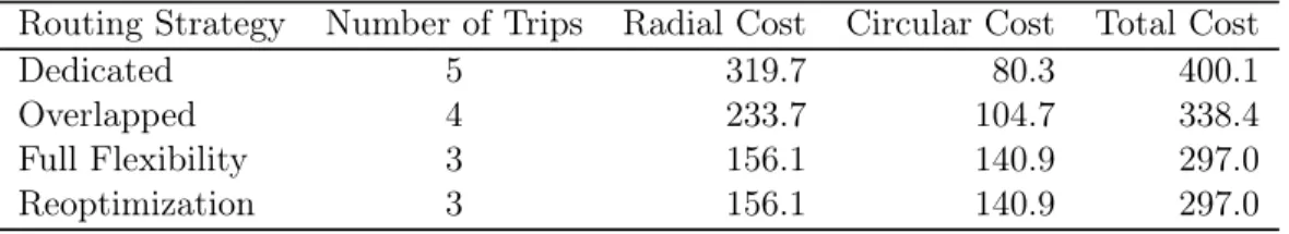
To summarize, Table 3.5 presents the outcomes for all routing strategies. In this table, radial cost is the total distance traveled to and from the depot while circular cost is the distance traveled between customers. Looking at the total cost (which equals the sum of the radial and circular costs), full flexibility and reoptimization are tied as the lowest cost strategies while dedicated routing is the most expensive. We also see that total cost increases with trip count, which drives the radial cost component. Here, radial cost makes up 53% of total cost for full flexibility and reoptimization, 69%
Figure 3.7: Reoptimized routes once demands are known in the example problem. Red labels state the demand filled with each trip.
for overlapped routing, and 80% for dedicated routing. The value of both overlapped and fully flexible routing over dedicated routing is that drivers can harness surplus capacity in the fleet to potentially eliminate the need for a refill trip elsewhere in the system. Additionally, even with a fixed sequence of customers, full flexibility matches the cost of reoptimization while still allowing for some consistency and early preparation. Therefore, fixed yet flexible routing can be a valuable strategy in settings where reoptimization is not logistically or computationally practical.
Finally, in comparing the flexible strategies, full flexibility outperforms overlapped routing but likely requires additional investment. For example, each driver must be prepared to travel over any part of the giant tour, and each customer must be willing to receive deliveries from different vehicles each day. Thus, overlapped routing can be a practical middle ground strategy with substantial gains – in this example, through a 15% savings – over the dedicated approach. Even more, we will see in Section 4 that overlapped routing actually performs comparably to full flexibility on average across several location and demand instances.
Routing Strategy Number of Trips Radial Cost Circular Cost Total Cost
Dedicated 5 319.7 80.3 400.1
Overlapped 4 233.7 104.7 338.4
Full Flexibility 3 156.1 140.9 297.0
Reoptimization 3 156.1 140.9 297.0
3.3
Asympototic Performance
Finally, though this thesis focuses on smaller scale problems, we briefly comment on the asymptotic characteristics of overlapped routing. Ledvina et al. (2020) use probabilistic analysis to derive a theoretical guarantee on the relative performance of overlapped routing as the number of customers approaches infinity. Specifically, they
find that given a demand distribution 𝐷𝑖 with mean 𝜇, then
lim 𝑁 →∞ 𝑍(𝑂) 𝑍* = lim𝑁 →∞ 𝑄𝑟𝑎𝑣𝑔 𝑁′𝜇 (3.1)
where 𝑍* is the optimal travel distance in expectation, 𝑍(𝑂) is the expected travel
distance under overlapped routing, and 𝑟𝑎𝑣𝑔 is the expected number of trips per
vehicle under overlapped routing. Additionally, if capacity 𝑄 is no more than a
route’s expected demand 𝑁′𝜇, then
lim 𝑁 →∞ 𝑍(𝑂) 𝑍* ≤ 1 + 𝜎 2𝜇√𝑁′ (3.2)
where 𝜎 is the standard deviation of demand. Excitingly, Equation 3.2 states that as the number of customers is scaled to infinity, the cost of overlapped routing relative to the optimal cost is bounded above by some constant. In other words, there is a cap on how much more costly overlapped routing will be in large scale problems. Even more, as either (i) the coefficient of variation of demand decreases and/or (ii) the size of a vehicle’s route increases, the bound becomes tighter and overlapped routing approaches reoptimization in cost. These theoretical guarantees are distribu-tionally robust, meaning they hold for any demand or customer location distribution, assuming the distributions are independent and identical across customers.
Chapter 4
Computational Study
We use numerical simulation to assess the cost-saving potential of the overlapped routing strategy. This chapter describes the simulation setup and presents the results for a baseline scenario along with some variations on the baseline as a sensitivity anal-ysis. Though we focus on the relative performance of overlapped routing, dedicated routing, and reoptimization, we also provide results for full flexibility, which we find closely aligns with overlapped routing.
4.1
Simulation Setup
In this study, we compare costs of the routing strategies from Chapter 3 under various network designs. Cost is measured as the total Euclidean distance traveled by the vehicle fleet in serving all customer demands. For each instance and routing strategy, the simulation program returns the total cost as well its radial and circular cost components. Recall that radial cost is the cumulative distance traveled to and from the depot (at the beginning or end of a route or when conducting a refill trip) while circular cost is the cumulative distance traveled between customers.
We simulate problems with 𝑁 = 5, 10, 20, 40, and 80 customers. For each problem size, we randomly generate 30 customer location instances and 200 demand instances. Customer demands are independently and identically distributed according to the demand scenario as defined in the following sections.
To create the a priori routes for each customer location instance, we first generate a traveling salesman tour through all customer locations. We then create extended routes beginning with the first customer in the tour’s sequence and calculate the total cost of overlapped routing over all demand instances. We rotate the tour to test each customer as the first customer in the tour’s sequence, and ultimately, keep the sequence that yields the lowest average overlapped routing cost. We use this sequence to generate the a priori routes used in the dedicated and overlapped strategy for all demand instances and that particular customer instance.
Simulations are run in Python 3.7. We use Google Optimization Tools (OR-Tools) (Perron and Furnon 2019) to (i) generate the traveling salesman tour used to create the a priori routes and (ii) solve the VRP with splittable demands for each demand instance. More specifically, for the VRP in each demand instance, we transform the integer demand problem into an equivalent problem with smaller customers each with unit demand and then find the optimal vehicle routes using the OR-Tools VRP solver. In the next section, we define our main scenario and describe the baseline simu-lation results. Unless specified otherwise, results for each problem size are presented as the average over all customer and demand instances.
4.2
Baseline Results
The main results in this study are for the baseline scenario, which has the parameters below:
• Demand 𝐷𝑖 ∼ Uniform{0, 8}, meaning that realized demand 𝑑𝑖 for each
cus-tomer 𝑖 equals 0, 1, 2, ..., or 8 with equal probability.
• Route size 𝑁′ = 5, meaning that the a priori primary route for each vehicle 𝑗
has 5 customers.
• Overlap size 𝑘 = 5 for each vehicle 𝑗, meaning that the a priori extended route
for each vehicle 𝑗 ̸= 𝑀 has 10 customers.1
• Vehicle capacity 𝑄 = 20 so that in expectation, vehicle 𝑗 can fully serve its primary route in a single trip.
Table 4.1 presents the total cost for each routing strategy in the baseline scenario while Figure 4.1 illustrates these results. We include both total cost and the cost relative to reoptimization. As the number of customers grows from 𝑁 = 5 to 𝑁 = 80, dedicated routing increases from 14% more expensive than reoptimization up to 26% more expensive. Overlapped routing, on the other hand, decreases from 14% more expensive than reoptimization at 5 customers down to just 6% more expensive at 80 customers. Ultimately, for 80 customers, we find that overlapped routing yields a 16% savings over dedicated routing on average.
Cust. Total Relative to Reoptimization
Dedic. Overlap. Full Flex. Reopt. Dedic. Overlap. Full Flex.
5 228.7 228.7 228.7 200.3 1.142 1.142 1.142
10 393.4 387.1 387.1 331.8 1.186 1.167 1.167
20 656.0 619.7 621.7 549.4 1.194 1.128 1.132
40 1,148.1 1,027.9 1,028.0 939.4 1.222 1.094 1.094 80 2,069.9 1,746.2 1,734.5 1,646.6 1.257 1.060 1.053
Table 4.1: Average cost in the baseline scenario
Full flexibility performs almost identically to overlapped routing, though inter-estingly, overlapped routing actually slightly outperforms full flexibility in problems with 10 customers. While intuitively more flexibility should enable lower costs, our fixed giant tour combined with randomness in the relatively few customer location instances means that full flexibility is not guaranteed to outperform overlapped rout-ing. Unsurprisingly, however, the random cost differences even out as customer size grows so that by 80 customers full flexibility does ultimately yield the lower average cost.
To look beyond average performance, Figure 4.2 shows the distribution of costs over all demand and customer instances. The figure includes one graph for each routing strategy, with each graph plotting a histogram of costs for problems with 5,
Figure 4.1: Average cost in the baseline scenario presented as (a) total cost and (b) cost relative to reoptimization
20, and 80 customers. We observe that the histograms roughly resemble a normal distribution. For simulations with 80 customers, dedicated routing exhibits a median of 2,060 and standard deviation of 175 while overlapped routing yields a lower median and standard deviation of 1,741 and 117, respectively. These results suggest that overlapped routing can decrease both the expected cost and the cost volatility of serving customers with stochastic demands.
We can also compare the performance of overlapped and dedicated routing for a given instance. Table 4.2 lists the percent of instances in which overlapped routing costs (i) more than, (ii) less than, and (iii) the same as dedicated routing. For instances with 5 customers, costs for dedicated routing and overlapped routing are always equal since the single extended route is identical to the primary route in the baseline scenario. However, for instances with 10 customers, overlapped routing is lower cost or higher cost with about equal probability. To explain the cases with higher cost, a vehicle 𝑗 = 1 may travel extra distance to support customers shared with vehicle 𝑗 = 2, but in a network with only two primary routes, this extra travel might not offset any depot trips. Put differently, in small flexible networks, savings in radial cost may not offset any additional circular cost. Finally, with a problem size of 20 or larger, overlapped routing is very likely to yield a lower cost than dedicated
Figure 4.2: Histogram of routing costs in the baseline scenario
routing for any given instance, reaching near certain savings for networks with 80 customers.
To better understand the overlapped strategy’s cost-saving mechanism, we sepa-rate total cost into its radial and circular components, illustsepa-rated in Figure 4.3. Table 4.3 states the corresponding total costs as well as radial cost’s share of the total by routing strategy and problem size. We see that in the three strategies presented, the radial share of total cost increases with the number of customers. Under dedicated routing, for example, the radial cost share increases from 40% for 5 customers to
Customers Overlapped Routing (Relative to Dedicated Routing) Higher Cost Equal Cost Lower Cost
5 0% 100% 0%
10 46.2% 6.92% 46.9%
20 28.9% 0.03% 71.0%
40 7.95% 0% 92.0%
80 0.08% 0% 99.9%
Table 4.2: Percent of instances in which overlapped routing yields higher cost, equal cost, or lower cost compared to dedicated routing in the baseline scenario. Note: Rows may not sum to 100% due to rounding.
75% for 80 customers. The radial share for overlapped routing, on the other hand, increases from 40% to 64%, which with a lower total cost equates to a 28% radial cost savings relative to dedicated routing. Overall, the increasing radial shares suggest that trips to and from the depot drive transportation costs as network size grows.
Figure 4.3: Average circular and radial costs in the baseline scenario
We can alternatively can capture the radial cost savings through differences in the number of trips needed for the fleet to meet all customer demands. Table 4.4 presents the average trip counts for each problem size and strategy, including full flexibility. The trip count includes vehicles’ initial departures from the depot plus any refill trips. For problems with 5 and 10 customers, the fleet performs similar numbers of trips in all routing strategies. However, with 20 customers, dedicated routing requires roughly
Customers Dedicated Overlapped Reoptimization Total Radial Share Total Radial Share Total Radial Share
5 229 40% 229 40% 200 43%
10 393 50% 387 42% 332 43%
20 656 58% 620 47% 549 44%
40 1,148 68% 1,028 56% 940 49%
80 2,070 75% 1,746 64% 1,647 52%
Table 4.3: Average radial share of total cost in the baseline scenario
one more trip than does reoptimization. Then, dedicated routing requires about 3 additional trips for 40 customers and ultimately 6 additional trips for 80 customers. Meanwhile, overlapped routing almost matches full flexibility and reoptimization in trip count across all problem sizes. Figure 4.4 illustrates dedicated routing’s dramatic divergence from the other three strategies. Also, note that while full flexibility yields slightly fewer trips than does reoptimization (14.49 versus 14.52, respectively), full flexibility is still the higher cost strategy as reported in Table 4.1 above.
Routing Strategy Number of Customers
5 10 20 40 80
Dedicated 1.28 2.55 5.13 10.27 20.57 Overlapped 1.28 2.20 4.02 7.65 14.90 Full Flexibility 1.28 2.20 3.97 7.48 14.49 Reoptimization 1.28 2.20 3.97 7.48 14.52
Table 4.4: Average number of trips in the baseline scenario
Understandably, all strategies require increasing total costs to meet the demands of growing numbers of customers. However, the baseline analysis reveals that trips to and from the depot contribute to a growing share of total costs as the number of customers increases. We observe that both the overlapped routing and full flex-ibility strategies can partly mitigate the increasing radial cost since the customer sharing strategy sometimes prevent a refill trip elsewhere in the network. Even more, overlapped routing performs almost equally to full flexibility though their relative
per-Figure 4.4: Average number of trips in the baseline scenario
formance may vary with the scenario design. Finally, in comparing the fixed routing strategies to reoptimization, we see that dedicated routing becomes relatively more expensive while overlapped routing and full flexibility grow closer to reoptimization in cost. In fact, as discussed in Section 3.3, we know that for infinitely large problems, the ratio between overlapped routing and reoptimization does ultimately converge to a constant lower bound.
4.3
Scenario Analysis
To understand routing cost’s sensitivity to different network parameters, we also run simulations for the scenarios summarized in Table 4.5. These additional scenarios are defined as variations on the baseline scenario with changes to overlap size, vehicle capacity, route length, or demand distribution. In this section, we analyze outcomes for each type of parameter change and compare the additional scenario results to the baseline.
Scenario Route Size, 𝑁′ Overlap Size, 𝑘 Vehicle Capacity, 𝑄 Demand Distribution, 𝐷 Baseline 5 5 20 𝐷𝑖∼ Uniform{0, 8} Medium Overlap – 3 – – Small Overlap – 1 – – High Capacity – – 25 – Low Capacity – – 15 – Short Route 2 2 8 – Long Route 10 10 40 –
Binomial Demand – – – 𝐷𝑖∼ Binomial(8, 0.5)
Stochastic
Customers – – – D𝑖 =
{︃
0 w.p. 0.5 8 w.p. 0.5
Table 4.5: List of scenarios. Cells with dashes indicate the parameter is the same as in the baseline scenario.
Varying Overlap Size
We first analyze the effect of varying overlap size 𝑘 in the overlapped routing strategy. Recall that the overlap size refers to the number of customers shared between two adjacent vehicle routes. In the baseline, overlap size equals primary route size for
all vehicles, which means 𝑘 = 𝑁′ = 5, Then, the extended route for vehicle 𝑗 < 𝑀
under overlapped routing contains the 5 customers in primary routes 𝑗 and the 5 customers in adjacent primary route 𝑗 +1. However, in two new scenarios we consider a smaller overlap size, specifically 𝑘 = 3 (three shared customers out of 5) in the medium overlap scenario and 𝑘 = 1 (1 shared customer out of 5) in the small overlap scenario. The baseline, medium overlap, and small overlap scenarios differ only in their extended routes, so they should exhibit different overlapped routing costs but identical dedicated routing costs.
Table 4.6 presents the ratio of the average overlapped routing cost to the average dedicated routing cost. For 80 customers, overlapped routing achieves 8% savings over dedicated routing in the small overlap scenario. Savings increase to 12% with medium overlap and 16% with the full baseline overlap. In comparing these scenarios, we find that much of the baseline savings is achieved with just one overlapped customer. In
fact, for all problem sizes, the marginal savings decrease as overlap size increases from 𝑘 = 1 to 3 to 5. Intuitively, increasing the number of shared customers among vehicles likely increases coordination time and cost, so our finding that much of the gains from flexible routing can be achieved with minimal investment could be very important in practice.
Scenario Number of Customers
5 10 20 40 80
Small Overlap (𝑘 = 1) 1.00 0.99 0.98 0.95 0.92 Medium Overlap (𝑘 = 3) 1.00 0.99 0.96 0.91 0.88 Baseline (𝑘 = 5) 1.00 0.98 0.94 0.90 0.84
Table 4.6: Average cost of overlapped routing relative to dedicated routing in the small overlap, medium overlap, and baseline scenarios. Note: Ratios for all scenarios use the baseline scenario’s computed dedicated cost. Dedicated costs in the medium and small overlap scenarios show minor variation from randomness.
Varying Capacity
We next analyze the impact of different vehicle capacities. In the baseline scenario, we set vehicle capacity 𝑄 equal to the primary route’s total expected demand. There-fore, for primary routes with 5 customers each with demand uniformly distributed between 0 and 8 and equal to 4 in expectation, all vehicles have a capacity of 20 units. Now, for a low capacity scenario, we decrease capacity by 25% to 15 units and for a high capacity scenario, we increase capacity by 25% to 25 units. All other network parameters remain unchanged from the baseline scenario, so we can think of these scenarios as simply using smaller or larger trucks, respectively, to execute the same routes.
Table 4.7 presents the total routing costs for the low capacity and high capacity scenarios relative to the baseline. As the number of customers grows, relative costs for all routing strategies increase for the low capacity scenario but decrease for the
high capacity scenario.2 This result is expected since a smaller vehicle requires more
trips from the depot to serve the same amount of demand as a larger vehicle.
We also observe that overlapped routing almost matches the relative costs under full flexibility, and both flexible strategies moderate the effect of the low capacity and high capacity scenarios. For example, for most of the problem sizes, the cost of dedicated routing in the low capacity scenario relative to the baseline is higher than the cost of overlapped routing in the low capacity scenario relative to the baseline. Meanwhile, the cost of dedicated routing in the high capacity scenario relative to the baseline is lower than overlapped routing’s relative cost. These numbers suggest the value of flexibility is higher in settings where more trips are needed (e.g., when vehicles are low capacity), a finding consistent with our discussion in section 4.2 on customer sharing as a strategy to prevent refill trips and decrease radial cost.
Scenario Routing Strategy Number of Customers
5 10 20 40 80 Low Capacity Dedicated 1.12 1.13 1.16 1.19 1.21 Overlapped 1.12 1.11 1.14 1.16 1.19 Full Flexibility 1.12 1.11 1.14 1.16 1.20 Reoptimization 1.07 1.11 1.16 1.19 1.22 High Capacity Dedicated 1.01 0.93 0.91 0.88 0.87 Overlapped 1.01 0.95 0.91 0.90 0.89 Full Flexibility 1.01 0.95 0.92 0.90 0.88 Reoptimization 0.98 0.94 0.91 0.88 0.87
Table 4.7: Average cost in the high capacity and low capacity scenarios relative to the baseline scenario
Varying Route Size
We also test different numbers of customers for the primary routes. In the baseline
scenario, each primary route has 𝑁′ = 5 customers. We now create a short route
scenario in which each primary route has 𝑁′ = 2 customers as well as a long route
scenario in which each primary route has 𝑁′ = 10 customers. We also adjust other
network parameters to maintain relationships consistent with the baseline. Specifi-cally, for the short route we decrease overlap size to 𝑘 = 2 to equal the new primary route length, and we decrease vehicle capacity to 𝑄 = 8 to equal the new expected primary route demand. Conversely, for the long route scenario we increase overlap size to 𝑘 = 10 and capacity to 𝑄 = 40.
Figure 4.5 illustrates the radial and circular components of total cost for each scenario under our three main routing strategies as the number of customers grows. Across scenarios, total costs decrease as route length increases, with much of the savings coming from a decreasing radial cost since fewer vehicle trips are needed to serve the same number of customers. See Table 4.8 for average trip counts, including for full flexibility. Comparing strategies within scenarios, overlapped routing shows a lower radial cost but higher circular cost for a net decrease in total cost relative to dedicated routing. Reoptimization slightly outperforms overlapped routing and remains the lowest cost strategy in all scenarios.
Figure 4.5: Circular and radial costs by routing strategy in the long route, short route, and baseline scenarios
Scenario Routing Strategy Number of Customers 10 20 40 80 Baseline Dedicated 2.55 5.13 10.27 20.57 Overlapped 2.20 4.02 7.65 14.90 Full Flexibility 2.20 3.97 7.48 14.49 Reoptimization 2.20 3.97 7.48 14.52 Long Route Dedicated 1.22 2.45 4.90 9.84 Overlapped 1.22 2.15 4.01 7.60 Full Flexibility 1.22 2.15 3.99 7.50 Reoptimization 1.22 2.15 3.99 7.51 Short Route Dedicated 6.54 13.10 26.24 52.54 Overlapped 4.95 9.56 18.80 37.32 Full Flexibility 4.81 9.18 17.94 35.49 Reoptimization 4.82 9.19 17.95 35.53
Table 4.8: Average number of trips in the long route, short route, and baseline sce-narios
Other Demand Distributions
Lastly, we consider scenarios in which customers face alternate demand distributions. In the baseline scenario, customer 𝑖’s integer demands are uniformly distributed
be-tween 0 and 8, that is 𝐷𝑖 ∼ Uniform{0, 8}. In a second scenario, customers instead
exhibit binomially distributed demand with 𝐷𝑖 ∼Binomial(8, 0.5). Finally, we define
a stochastic customer scenario in which customers exhibit demand of 0 or 8 with equal probability. Note that all three of these scenarios assume customer demands
are independently and identically distributed with expected demand E[𝐷𝑖] = 4. The
demand variance is 5.33 in the baseline scenario, 2 in the binomial demand scenario, and 16 in the stochastic customers scenario.
Table 4.9 presents the total cost in each strategy, scenario, and problem size. For all routing strategies, we observe that the stochastic customer scenario is generally the lowest cost scenario, followed by the baseline scenario, and then the binomial demand scenario. Table 4.10 simply rearranges the costs from Table 4.9 to highlight the relative performance of overlapped routing within each scenario. In all scenarios,
overlapped routing almost perfectly matches the cost of full flexibility. We also ob-serve that overlapped routing approaches reoptimization in cost most rapidly in the stochastic customer scenario. Specifically, overlapped routing costs in the stochastic customer scenario decrease from 19% above reoptimization for 5 customers to 3% above for 80 customers, yielding a 16 point change. In comparison, relative costs decrease by 13 points under binomial demand and by only 8 points in the baseline.
Routing Strategy Scenario Number of Customers
5 10 20 40 80 Dedicated Baseline 229 393 656 1,148 2,070 Binomial Demand 266 436 745 1,308 2,330 Stochastic Customers 180 334 594 1,104 2,070 Overlapped Baseline 229 387 620 1,028 1,746 Binomial Demand 266 422 690 1,132 1,935 Stochastic Customers 180 324 546 958 1,697 Full Flexibility Baseline 229 387 622 1,028 1,735 Binomial Demand 266 422 691 1,133 1,934 Stochastic Customers 180 325 548 956 1,686 Reoptimization Baseline 200 332 549 939 1,647 Binomial Demand 226 365 611 1,052 1,845 Stochastic Customers 152 289 512 911 1,648
Table 4.9: Average cost in the binomial demand, stochastic customer, and baseline scenarios
Finally, for a more granular understanding of the demand scenarios, we can also compare performance for individual instances. Figure 4.6 shows the percent of de-mand and customer location instances in which overlapped routing costs the same, more, or less than dedicated routing. In all scenarios, overlapped routing is more expensive less than half of the time and more consistently becomes the less expensive strategy as the number of customers grows. Additionally, a greater share of instances see a higher cost for flexible operations when customer demands are uniform as in the baseline scenario. This observation aligns with the baseline’s higher relative costs as presented in Table 4.10.
Scenario Overlapped Cost Number of Customers
5 10 20 40 80
Baseline
Total 229 387 620 1,028 1,746
Rel. to Dedicated 1.00 0.98 0.94 0.90 0.84 Rel. to Full Flexibility 1.00 1.00 1.00 1.00 1.01 Rel. to Reoptimization 1.14 1.17 1.13 1.09 1.06 Binomial Demand
Total 266 422 690 1,132 1,935
Rel. to Dedicated 1.00 0.97 0.93 0.87 0.83 Rel. to Full Flexibility 1.00 1.00 1.00 1.00 1.00 Rel. to Reoptimization 1.18 1.16 1.13 1.08 1.05 Stochastic Customers
Total 180 324 546 958 1,697
Rel. to dedicated 1.00 0.97 0.92 0.87 0.82 Rel. to Full Flexibility 1.00 1.00 1.00 1.00 1.01 Rel. to Reoptimization 1.19 1.12 1.07 1.05 1.03
Table 4.10: Average total and relative costs of overlapped routing in the baseline, binomial demand, and stochastic customer scenarios
Figure 4.6: Percent of instances in which the cost of overlapped routing is equal to, higher than, or lower than the cost of dedicated routing in the binomial demand, stochastic customer, and baseline scenarios