• Aucun résultat trouvé

Regularized non-local Total Variation and application in image restoration

N/A
N/A
Protected

Academic year: 2021

Partager "Regularized non-local Total Variation and application in image restoration"

Copied!
22
0
0

Texte intégral

(1)

HAL Id: hal-01342111

https://hal.archives-ouvertes.fr/hal-01342111v3

Submitted on 11 Sep 2017

HAL is a multi-disciplinary open access

archive for the deposit and dissemination of

sci-entific research documents, whether they are

pub-lished or not. The documents may come from

teaching and research institutions in France or

abroad, or from public or private research centers.

L’archive ouverte pluridisciplinaire HAL, est

destinée au dépôt et à la diffusion de documents

scientifiques de niveau recherche, publiés ou non,

émanant des établissements d’enseignement et de

recherche français ou étrangers, des laboratoires

publics ou privés.

Regularized non-local Total Variation and application in

image restoration

Zhi Li, François Malgouyres, Tieyong Zeng

To cite this version:

Zhi Li, François Malgouyres, Tieyong Zeng. Regularized non-local Total Variation and application

in image restoration. Journal of Mathematical Imaging and Vision, Springer Verlag, 2017, 59 (2),

pp.296-317. �10.1007/s10851-017-0732-6�. �hal-01342111v3�

(2)

Noname manuscript No. (will be inserted by the editor)

Regularized non-local Total Variation and application

in image restoration

Zhi Li · François Malgouyres · Tieyong Zeng

Received: date / Accepted: date

Abstract In the usual non-local variational mod-els, such as the non-local total variations (NLTV), the image is regularized by minimizing an energy term that penalizes gray-levels discrepancy between some specified pairs of pixels, a weight value is computed between these two pixels to penalize their dissimilarity. In this paper, we impose some reg-ularity to those weight values. More precisely, we minimize a function involving a regularization term,

analogous to an H1 term, on weights. Doing so,

the finite differences defining the image regularity depend on their environment. When the weights are difficult to define, they can be restored by the proposed stable regularization scheme.

We provide all the details necessary for the im-plementation of a PALM algorithm with proved convergence. We illustrate the ability of the model to restore relevant unknown edges from the neigh-boring edges on an image inpainting problem. We also argue on inpainting, zooming and denoising problems that the model better recovers thin struc-tures.

Z. Li

Department of Computational Mathematics, Science and Engineering, Michigan State University, MI, USA

E-mail: zhi_li@life.hkbu.edu.hk. ZL is supported in part by the NSF grant DMS-1621798.

F. Malgouyres

University of Toulouse, CNRS, Toulouse, France, E-mail: Francois.Malgouyres@math.univ-toulouse.fr. T. Zeng

Department of Mathematics, Hong Kong Baptist Univer-sity, Hong Kong, China,

E-mail: zeng@hkbu.edu.hk. TZ is partially supported by NSFC 11271049, RGC 12302714 and RFGs of HKBU.

Keywords non-local regularization · proximal alternating linearized minimization · nonconvex minimization · total variation · image restoration Mathematics Subject Classification (2000) 49N45 · 65K10 · 90C26

1 Introduction

1.1 The Image Restoration Problem

Given an image domain P (P can be a sub-domain of R2), we consider a degraded image I as a

map-ping P → R. We assume that I is obtained from a

perfect unknown imageu by

I = Hu + b, (1)

where H is a known linear operator and b is an error term. In the typical situations we have in mind, P is a lattice of pixels and b is an iid noise with standard deviation σ > 0.

The purpose of the restoration model studied in this paper is to retrieve an image close tou, using only I and H. For instance, in image inpainting, the operator H maps any image u onto an image Hu satisfying

(Hu)p=

 0 , if p ∈ P0,

up, otherwise,

(2) where P0 is the domain to inpaint.

For deblurring, the operator H is typically the convolution operator. For the purpose of image zooming the operator H is the composition of a convolution and a subsampling operator (the lat-ter can also be written under the form (2)) and so on and so forth. Note that, to simplify notations,

(3)

we use the same domain P for the perfect image u and the measure I. This need not be the case in general.

Finally, for simplicity, we assume that P is pe-riodic, so that for any (p, q) ∈ P2the sum p + q is

defined in such a manner that p + q ∈ P. We also assume that P is such that p + P = P, whatever p ∈ P.

1.2 Review of Image Restoration Models

Total variation (TV) has drawn much attention since Rudin, Osher and Fatemi (ROF) proposed their celebrated model [39] for denoising (i.e. H = Id). The variational formulation can be written as argmin

u∈Ω

|∇u| + λku − Ik2, (3)

where Ω is either RP (in the discrete setting) or the space of the functions of bounded variation. When used as a regularization term, the total variation |∇u| has the advantage to preserve sharp edges and the drawbacks to create homogeneous regions (staircasing) and to over-smooth the textured re-gions. This is due to the fact that textures are treated as singularities by the TV term which only sees local information [25]. This regularization has later been used to solve many linear inverse prob-lems such as inpainting [5, 41].

In another direction, generalizing the Yaroslavsky neighborhood filter [47], the non-local means (NLM) of Buades, Coll and Morel [8] takes the following form (we write it in the continuous domain): N LMI(p) = 1 C(p) Z B vI(p, p0)I(p0)dp0, (4)

where B is a search window, the weights are pro-vided by vI(p, p0) = exp  −D(p, p 0) h2  , (5)

where, for a patch ˆB (usually a square centered around the origin),

D(p, p0) = Z ˆ B Ga(q) |I(p + q) − I(p0+ q)| 2 dq (6)

and the normalizing factor C(p) =

Z

B

vI(p, p0)dp0. (7)

The Gaussian kernel Ga with standard deviation

a ponderates pixels in the ’patch’ area and h is a filtering parameter. Usually in NLM model, the

patch is nothing but a square region which is smaller than the search window B. The idea behind NLM is to restore the pixel in the contaminated image I by a weighted average of the nearby similar (in the patch sense) pixels. The patch is used to judge the resemblance between two pixels p and p0, in (6), D(p, p0) is evaluated based on the difference of the square neighborhoods (patches) I(p + q) and I(p0 + q) centered at p and p0, not the intensity difference between the pixels p and p0 themselves. Another key point is that the pixels p0 used in the average do not have to be close to p, which explains the name ’non-local’.

The idea to use patch was initially known for its ability to do ’texture synthesis’ [30, 44], it was later applied to image denoising and inpainting [1]. Patch is widely used in image processing models. For example, Pizarro, et al. [38] used a linear com-bination of a similarity term and a smoothness term, both of them are defined non-locally in a patch manner to propagate nonlocal information. NL-Bayes [28, 29] bridges between the Bayesian methods and BM3D. It improves the denoising re-sult, when applied to color images and, for gray level images, yields to results comparable to state-of-the-art methods, such as BM3D.

From a weighted graph point of view, Kher-admand and Milanfar [27] proposed an adaptive Laplacian filter using patch, which is mainly for deblurring, and under special circumstances, their method can apply to denoising and sharpening problems. Notice that a similar idea, coming with a precise statistical analysis, has been proposed un-der the name "Discrete Universal Denoiser" [46].

Considering a thin structure (typically a smooth curve) in a uniform background, we see in the for-mula that the weights vIdoes not differentiate well

the pixels in the thin structure from pixel in the background. The thin structure indeed lives in a domain whose measure is small (at the limit, the measure of the domain is 0). It provides a negligible contribution to D(p, p0). As a consequence, NLM tends to underestimate the weights of the pixels in the thin structure and, as a consequence, it tends to erase the thin structure. This is especially true for large patch size and may lead to a substan-tial underestimation of the similarity between two pixels in the thin structure [18].

Moreover, exemplar-based approaches [30, 44] also use patches to produce striking inpainting re-sults. These algorithms have been later interpreted using a probabilistic point of view. In particular, Levina and Bickel [30] provided a theoretical

(4)

back-ground to explain their ability to synthesize tex-ture. Aujol, Ladjal and Masnou [4] expressed the exemplar-based methods in a non-local variational framework and studied their ability to retrieve ge-ometric features. However, it is difficult to adapt NLM and other patch based approaches for diffi-cult image restoration tasks involving highly struc-tured noise or (even worse) when the operator H is not invertible and makes the recovery of similar pixels difficult.

Inspired by the advantages of NLM, Gilboa and Osher [23, 24] introduced a non-local variational model to better recover textures. In [24], they con-sidered the non-local total variation (NLTV) model defined (in the continuous domain) by

JN LT V(u) + λku − Ik2, (8)

where the NLTV term JN LT V(u) is defined by

Z P s Z B (u(p) − u(p + q))2v(p, q)dqdp. (9)

In [24], in practical applications, they calculated the weights v according to patch distance and only used the 10 most similar pixels in (the discretized) B. They also mentioned binary weights. They adapted the celebrated Chambolle’s projection algorithm [10] to optimize a discretization of the NLTV model. A more general model, involving p-Laplace opera-tor on graphs, have been proposed in [19]. It also makes connections between the variational approaches and other non-local approaches.

Considering applications such as compressive sensing, when the low sampling rate may lead to a bad initial guess of the weight function, some authors [37, 48] suggested to update the weights during the iterations to improve them. For exam-ple, Zhang, et al. [48] employed patches and up-dated the weights by recomputing the initial step (5) with the current estimate of the clean image. A similar update is used in [1, 37]. To trade off be-tween the accuracy and computational costs, the authors only reevaluate the weights every few steps [48] and in practical implementation, they only use the first few largest weights in a local search win-dow and set the rest of them to zero. Of course, because of these last ’tricks’, the algorithms may fail to find the optimal solution of the variational model which is not fully satisfactory. They however provide interesting restoration results.

The model studied in this paper is inspired by the earlier work of Peyre, et al. [36, 37]. In [36], they considered the weights v defined in the NLM and updated v using (5) with the current estimate

of the image. The authors mentioned the difficulty for setting the filtering parameter h [36] since noise level evolves along the iterative process. In [37], the authors extended [36] and [48] by regularizing the graph v. The resulting model has two regular-ization terms, the first term Jv(u) regularizes the

image, while the second term E(v) is the entropy of function v defining the underlying graph. Also, to better recover the textures of the images, the non-local regularization term was chosen to be the patch variation of JN LT V(u) in (9). In this

varia-tion, the difference of intensities u(p) − u(p + q), in (9), is replaced by a patch distance. It has also been adopted in [1, 20, 35].

To conclude, non-local variational models [17, 24,31,37] have been widely used to restore images, because of their capability to utilize the informa-tion from many pixels having a similar neighbor-hood. However, when treated by these models, thin structures can be overlooked and are sometimes undetectable in a patch of the damaged image. These methods might therefore erase these thin structures.

Also, the construction of the weights between the pixels is usually done according to some pixel similarity criterion in the degraded images I. When some weights are unknown (for instance when in-painting a missing domain or zooming an image), they are updated during the iterative process, ac-cording to an ad-hoc procedure [37]. More gener-ally, these methods are difficult to apply and lack precise modeling when the output of the degrada-tion operator H does not look like an image (think about the restoration an image from random mea-surements or Computerized Tomography.)

When compared to these methods, the model studied in this paper is a regularized non-local to-tal variation (RNLTV) model. It shows the advantages to both: better restore thin structures; -allow the construction of non-local models for dif-ficult inverse problems.

1.3 The Studied Model

1.3.1 Framework and Model Description

From now on, we discretize the problem and con-sider a lattice P. We concon-sider a set B ⊂ P. In the typical situation we have in mind, B is a square centered at the origin with radius1 r. Throughout the paper, we call patch or window a set p + B for some p ∈ P.

(5)

We also denote the cardinality of any finite set C by |C|. Moreover, for any finite dimensional vec-tor space V (in practice we have either V = RP, V = RP×B or V = RB) and any positive definite operator L mapping V into itself, we consider the weighted norm [15]

kxkL = hx, Lxi

1

2, ∀x ∈ V, (10)

where h., .i denotes the usual scalar product in V . When L is an identity matrix (L = Id), we simply denote kxk instead of kxkId.

Given these notations, we define, for any p ∈ P, weights vp = (vpq)q∈B ∈ RB, where each weight vqp

is the cost for the dissimilarity |up− up+q|. Said

differently, vp∈ RB can be seen as the parameters

of a finite difference operator defined at the pixel p. In practice we will force these weights vp∈ RB

to belong to the set

U =    v ∈ RB+, X q∈B vq = 1    , (11)

where R+ are the non-negative reals. This

con-straint guarantees that every pixel of the image contributes similarly to the overall cost. We de-note the collection of all the weights in the image by v = (vp)

p∈P∈ UP.

Given v, we define the non-local total variation of u ∈ RP by T V (v, u) =X p∈P Ψµ   s X q∈B vpq(up− up+q)2  , (12)

where µ > 0 and Ψµis the Moreau envelope of the

absolute value function, also called Huber function [6, page 368]: ψµ(t) = ( |t| −µ2 , if |t| ≥ µ, t2 2µ , otherwise. (13)

Note that (9) is a continuous analogue of (12) with-out the Huber function Ψµ. The first motivation for

using the Huber function is that, once the weights are properly estimated, we expect vp

q to be small

when (up−up+q)2is large. As a consequence, we do

not expect edges to be oversmoothed and blurred. As a consequence, the benefit of the `1 term used

to define the total variation might be questioned and it is interesting to use a function Ψµ, involving

a parameter µ, that permit Ψµto behave

quadrat-ically or linearly. The second motivation for using the Huber function is that it is differentiable. This

is required by the PALM algorithm. Moreover, we consider, for any v ∈ UP, the regularity criterion R defined by R(v) = γ X p∈P X p0∈N kvp− vp+p0k2, (14)

where γ is a non-negative parameter and N is a

small neighborhood2 of 0. When minimized, the

term R(v) favors the situation when vp is similar

to vp+p0. If we isolate vp

q in T V (v, u) + R(v), we

observe that vqpshould minimize

Ψµ   s X q0∈B vpq0(up− up+q0)2  +γ X p0∈N (vqp−vp+p0 q ) 2. As a consequence, vp

q must be small when (up−

up+q)2is large and must be similar to the weights

at its neighbor vp+pq 0. Also, since v ∈ UP, the T V (., u) term forces vp

q to be large for p and q such

that (up−up+q)2is small. For instance, when p and

p+q are on the same side of an edge or in the same thin structure; we know that (up− up+q)2is small;

it does not cost much to have vp

q large (i.e. close to

1). Although it depends on the local structure in the image, we also often have (up+p0 − up+p0+q)2 small and therefore vp+p0

q large. Altogether, we

ex-pect v to end up aligned with such edges and thin structures. This looks like a desirable behavior.

Finally, we consider a data fidelity term D. This term either takes the form

D(u) = λkHu − Ik2, (15)

for some parameter λ ≥ 0, or, for a parameter τ ≥ 0,

D(u) = χ|kHu−Ik2≤τ(u), (16)

where the indicator function χ|C is 0 if the

con-dition C is satisfied and infinity otherwise. The advantage of the latter formulation is that τ can be deduced from the noise standard deviation σ (A standard choice is indeed τ = |P|σ2).

The restored image we are interested in is the argument u of a minimizer of

argmin

u∈RP,v∈UP

R(v) + T V (v, u) + D(u). (17)

Although the parameters are not presented explic-itly in (17), the model depends on the parameters µ, γ and either λ or τ .

2 In the experiments, we consider4-connectivity: N =

(6)

Notice that, the model does not make use of the patch distance. It can therefore be categorized as a purely non-local method.

In the problem (17), the constraint on v is com-pact and, unless in very particular counter-example, we expect the objective function to be coercive in u. The objective function being also lower semi-continuous, the problem (17) has a solution. We will see moreover that T V and R are differentiable and have Lipschitz gradient (see Proposition 1, 2 and 3). The main difficulty concerning the numer-ical resolution of (17) is that, because of the term T V (u, v), the objective function is not convex.

1.3.2 Insight on the Model

The connectivity principle [26, 32] states that hu-man prefers to see that disjoint edges are con-nected through the missing domains. It is well-known that the classic inpainting models including TV models [5,41], have difficulty in connecting the thin objects [11,12] (see Figure 1, ’TV’ inpainting). Thus inpainting methods involving higher order information [11, 40], such as curvature, were pro-posed to improve the results. However, if the size of the unknown regions separating thin objects are too large, then even the fourth-order PDE-based model [40] will leave the thin structures broken (see Figure 1, ’TV-H−1’ inpainting).

Moreover, we see on Figure 1, ’NLinpaint’ im-age, that even non-local methods that do not struct v with enough care [21] have difficulty con-necting lines, when there are many large missing areas. One motivation for considering RNLTV is that, because it smoothly inpaints v in the missing regions and since large weights values are concen-trated and aligned along the direction of the thin structures, RNLTV has the ability to connect the broken lines.

1.4 Overview of the Paper

In Section 1.3, we present the RNLTV model. Sec-tion 2 details the proximal alternating linearized minimization (PALM) algorithm [7] minimizing the proposed model. We also provide in this section the gradient of the different terms, show that the gra-dients are Lipschitz continuous and provide their Lipschitz constants. The numerical experiments in Section 3 demonstrate the efficiency of the pro-posed method on inpainting, zooming and denois-ing experiments.

clean polluted

TV TV-H−1

NLinpaint RNLTV

Fig. 1 A synthetic image with thin lines contaminated by11×11missing squares. All methods fail to follow the Connectivity Principle properly, but RNLTV can connect the broken thin lines.

2 Implementing the PALM Algorithm In the last couple of years, alternating minimiza-tion algorithms [3, 7, 13, 14, 15, 34] were developed to solve optimization problems over multiple vari-ables. A proof of convergence in the non-convex setting for an alternating variant of the forward-backward algorithm, tagged PALM, has been pro-posed in [7]. It is perfectly adapted to the structure of (17). A preconditioned version has also been studied in [15].

Below, we provide the details for implementing the PALM algorithm generating a sequence that converges to a stationary point of (17). First, we give a few notations and describe the algorithm in Section 2.1. Next, we derive the components of the algorithm. Section 2.2, 2.3 and 2.4 are devoted to the calculation of the gradients of the regulariza-tion terms in (17) and their Lipschitz constants. Then we discuss the proximal operator proxD

L (u0)

in Section 2.5 in detail.

2.1 Notations and Overview of the Algorithm We denote ∇uT V (v, u) and ∇vT V (v, u) as the

partial gradient of T V (., .) with regards to the variable u and v respectively. The PALM algo-rithm adapted to (17) is described in Algoalgo-rithm 4.

(7)

In summary, the Algorithm 4 alternates forward-backward iterations for each one of the two block of variables: u and v.

For any v ∈ UP and any u ∈ RP, we assume

that we know a linear operator L and constants l and l0 (for the detailed calculations of these quan-tities see Section 2.2, 2.3 and 2.4) satisfying the majorization conditions [15] described below:

– For any v ∈ UP, L is such that there exists m > 0 satisfying

kukL≥ mkuk, ∀u ∈ RP, (18)

and for any u and u0∈ RP

T V (v, u0) ≤ T V (v, u) + h∇uT V (v, u) , u0− ui +1 2hu 0− u, L(u0− u)i . (19)

– For any u ∈ RP, l ≥ 0 and l0≥ 0 are such that l + l0 > 0 and for any v and v0 ∈ UP

T V (v0, u) ≤ T V (v, u) + h∇vT V (v, u) , v0− vi + l 2kv 0− vk2 , (20) and R(v0) ≤ R(v) + h∇R(v), v0− vi +l 0 2kv 0− vk2. (21)

Moreover, the proximal operators used in Al-gorithm 4 are defined, for any u0∈ RP, by

proxDL(u0) = argmin u∈RP D(u) +1 2ku − u 0k2 L, (22)

and for any v0∈ UP,

proxχ|U P(v0) = argmin

v∈UP

kv − v0k2, (23)

simply is the orthogonal projection onto UP. Given the above quantities l, l0 and L, the Al-gorithm 4 has many advantages and is perfectly adapted to the structure of our problem. The lat-ter indeed satisfies the following properties:

1. The objective function is analytical and satis-fies the KL property.

2. R(v), T V (v, u) and D(u) are proper, non-negative and lower semi-continuous.

3. The partial gradients ∇uT V (v, u) and ∇vT V (v, u)

are Lipschitz continuous with bounded moduli.

Algorithm 1: Overview of the algorithm

Input:

I: Degraded image

H: Linear operator to invert B: Support of the weights

N : Support for the finite differences defining R γ, µ, λ/τ : parameters

Output: u: Restored image v: Weights begin

Initialize the image u and v; while not converged do

step 1: Update u: u= proxD L u − L −1 uT V(v, u) (24) step 2: Update v: v= proxχ|U P v −∇vT V (v,u)+∇R(v) l+l0 

4. The sequence generated from Algorithm is bounded since both u and v are belong to compact sets. It is shown in [7, 15] that the sequence gener-ated by (even an inexact version of) Algorithm 4 has good convergence properties:

– The objective function decays along the itera-tive process.

– The iterates converge to a stationary point of our problem.

– The sum over the iterative process of the dis-tance between two successive iterates is finite. Of course, calculating the Kurdyka-Lojasiewicz characterization of our objective function would provide a better understanding of the convergence quality but it is not the purpose of the paper.

Finally, in order to implement the algorithm, we need to

– compute ∇uT V (v, u) and construct the

oper-ator L satisfying (19) (see Section 2.2); – compute ∇vT V (v, u) and the constant l

satis-fying (20) (see Section 2.3);

– compute ∇R(v) and the constant l0 satisfying (21) (see Section 2.4);

– compute the proximal operator (22) (see Sec-tion 2.5);

– compute the proximal operator (23): Notice that this reduces to multiple projections onto a sim-plex. The latter projection is a well studied problem for which fast algorithms exists [16].

(8)

2.2 Calculation of ∇uT V (v, u) and L

For any v ∈ UP, we consider the following non-local analogue of the finite difference operator:

Dv : RP −→ RP×B u = (up)p∈P 7−→  pvp q (up− up+q)  (p,q)∈P×B (25) We also denote, for p ∈ P,

(Dvu)p= ((Dvu)p,q)q∈B∈ RB

and k(Dvu)pk =

q P

q∈B(Dvu)2p,q.

We obtain after some simple calculations that its adjoint is given, for any w = (wp,q)(p,q)∈P×B, it

is easy to see that

(D∗vw)p= X q∈B q vpq wp,q− q vqp−q wp−q,q  , (26) for all p ∈ P.

Moreover, if we consider, for w ∈ RP×B, the norm

kwk∞,2= max

p∈Pkwpk, where wp= (wp,q)q∈B∈ R B.

(27) We can prove (see appendix 5.1) that for any u ∈ RP and any (fixed) v ∈ UP

T V (v, u) = max kwk∞,2≤1 hDvu, wi − µ 2kwk 2. (28)

From this expression and using the Theorem 1 in [33] (reminded in Appendix 5.2), we can deduce the following proposition whose proof is detailed in Appendix 5.2. Notice that a similar statement and construction is given for the usual total variation in [45].

Proposition 1 For any u ∈ RP, we have

∇uT V (v, u) = D∗vw∗(u), (29)

where w∗(u) ∈ RP×Bis the maximizer of (28) and is provided in closed form by:

w∗(u)p,q = ((Dvu)p,q µ , if k(Dvu)pk ≤ µ, (Dvu)p,q k(Dvu)pk , otherwise. (30)

Moreover, u → ∇uT V (v, u) is Lipschitz

continu-ous with Lipschitz constant l” =

2p|B| + 1

µ . (31)

As a consequence, we have for any u and u0∈ RP

T V (v, u0) ≤ T V (v, u) + h∇uT V (v, u) , u0− ui +l” 2ku 0− uk2. (32)

A straightforward consequence of (32) is that for any diagonalizable linear operator G whose eigen-values are all larger than 1 (and in particular for G = Id), the property (19) holds for L = l”G.

2.3 Calculation of ∇vT V (v, u) and l

Let us first define, for any fixed u ∈ RP, the linear operator Au: RP×B−→ RP, (vp,q)(p,q)∈P×B7−→  P q∈Bvp,q(up− up+q) 2 p∈P . (33) The interest for this operator comes from the fact that for any v ∈ UP

T V (v, u) =X p∈P Ψµ q (Auv)p  . (34)

Notice that, when v ∈ UP, we have for any p ∈ P

(Auv)p≥ 0. (35)

We easily obtain that the adjoint A∗uof Auis given

for any w ∈ RP by

(A∗uw)p,q= wp(up− up+q)2, ∀(p, q) ∈ P × B.

(36) Using these notations, we can prove (see Ap-pendix 5.3) the following proposition.

Proposition 2 For any fixed u ∈ RP, we have for any v ∈ UP

∇vT V (v, u) = A∗uu∗(v), (37)

where for all p ∈ P

(u∗(v))p= ( 1 2√(Auv)p , if p(Auv)p≥ µ, 1 2µ , if µ >p(Auv)p≥ 0. (38) Moreover, the function v 7−→ T V (v, u) is concave over RP×B+ and (20) holds for l = 0.

(9)

2.4 Calculation of ∇R(v) and l0

Let us first define the linear operator B: RP×B−→ RP×B×N,

(vp,q)(p,q)∈P×B7−→ (vp,q− vp+p0,q)

(p,q,p0)∈P×B×N. (39) We immediately deduce from (14) that for any

v ∈ RP×B

R(v) = γ kBvk2. (40)

We also easily obtain that the adjoint B∗ of B is

provided for any w ∈ RP×B×N by

(B∗w)p,q=

X

p0∈N

wp,q,p0−wp−p0,q,p0, ∀(p, q) ∈ P × B. (41) We can now state the following proposition whose proof is provided in Appendix 5.4.

Proposition 3 For any v ∈ UP, we have

∇R(v) = 2γB∗Bv. (42)

Moreover, v → ∇R(v) is Lipschitz continuous with Lipschitz constant 6√2γ|N |. As a consequence, (21) holds for l0= 6√2γ|N |.

2.5 Calculation of proxD L(u0)

Below, we provide closed form expressions that

permit to compute proxD

L (u

0) for the two data

fi-delity terms considered in this paper. In the de-noising case, H is a identity; for the purpose of image inpainting, H multiply every entry of the image by either 1 or 0 (see (2)).

– When D(u) = λku − Ik2 and L = l”Id.

In this case, we want to compute proxλku−IkL 2(u0) = argmin u∈RP λku − Ik2+l” 2ku − u 0k2, = 2λ 2λ + l”I + l” 2λ + l”u 0.

– When D(u) = χ|ku−Ik2≤τ(u) and L = l”Id.

In that setting, we have proxχ|ku−Ik2 ≤τ L (u 0) = argmin u:ku−Ik2≤τ ku − u0k2 L = ( u0 , if ku0− Ik2≤ τ, I + √ τ ku0−Ik(u0− I) , otherwise.

– When D(u) = λkHu − Ik2

In this case, proxλkH.−IkL 2(u0) = argmin u∈RP λkHu − Ik2+l” 2ku − u 0k2, = u∗,

where for all p ∈ P

• if H is defined by (2) for some fixed subset of pixels P0⊂ P u∗p= ( u0p , if p ∈ P0, 2λIp+l”u0p 2λ+l” , otherwise. (43)

• if H is a general linear operator (e.g. the subsampling operator used for zooming) then the solution u∗ of

2λHT(Hu − I) + l” (u − u0) = 0, (44)

can be computeded by the conjugate gradi-ent (CG) method for a sparse linear equa-tion of the form

Au = b, (45)

where A = 2λHTH + l”Id and b = 2λHTI+

l”u0. Note that, although we use CG (call Matlab function pcg(A,b)) to solve this sub-problem, the elementwised max norm of the residual max |Au∗− b| is around 10−13.

3 Numerical experiments

In order to illustrate the behavior of the model, we consider in this section three applications: im-age inpainting, zooming and denoising. We evalu-ate the ability of the method to restore both syn-thetic and natural images with a particular em-phasis on the restoration of thin structures. We compare the performance of the proposed RNLTV model with the performance of state of the art methods. We also illustrate how the weights v are adjusted once the convergence has been reached using the Isotropy Map described in Section 3.1 and 3.2. Finally, Section 3.3 is devoted to the in-painting experiments, Section 3.4 presents zoom-ing results and Section 3.5 contains the experi-ments on the denoising problem.

Notice that we have used the different data-fidelity terms mentioned in Section 1.3.1. They all show similar computational cost and convergence properties. For completeness, we summarize the data fidelity term chosen for each experiments in Table 1.

(10)

Table 1 The different data-fidelity terms used in the ex-periments.

D(u)

inpainting and zooming λkHu − Ik2

denoising (synthetic image) χ|ku−Ik2≤τ(u)

denoising (natural image) λku − Ik2

(−5,5) (−4,5) ... (4,5) (5,5) (−5,4) (−4,4) ... (4,4) (5,4) . . . ... ... ... (−5,−4) (−4,−4) ... (4,−4) (5,−4) (−5,−5) (−4,−5) ... (4,−5) (5,−5)

Fig. 2 The window B of size11×11. Every q ∈ B has a coordinate.

3.1 The Isotropy Map

To represent the distribution of the weights v, we

introduce the isotropy map M (v) ∈ RP. At

ev-ery pixel p ∈ P, the feature M (v)p represents

whether the weights in vp are distributed

isotrop-ically or not. Intuitively, the distribution is not isotropic when the significant weights are concen-trated along a thin region of the window p + B. The feature therefore needs to reflect the discrep-ancy between the projections of vp onto two axes one of which is aligned with the orientation of vp,

the other being orthogonal. Notice that the dis-crepancy is maximal when the coordinate system is aligned with the orientation of vp.

3.1.1 Implementation Details

More precisely, given an angular precision

param-eter K ∈ N 3 we define the small angle θ = π

2K

as shown in Figure 3. Then we consider all the co-ordinate (x, y) clock-wise rotated by an angle mθ, for m ∈ M, with M = {0, 1, 2, . . . , K − 1}. Doing so, we get several orthonormal bases denoted by im= (sin(mθ), cos(mθ)),

jm= (cos(mθ), − sin(mθ)).

3 In the experiments, we use K= 90.

Fig. 3 Coordinate change and projection of the weights on the new coordinate system.

We remind that any pixel q ∈ B is represented in the basis (im, jm) by the coordinates

(hq, imi, hq, jmi). (46)

Therefore, the average distance to the origin of the projections of vp onto the axes i

m and jm are

de-fined by Pmx =X q∈B vpqhq, imi , (47) Pmy =X q∈B vpqhq, jmi . (48)

The isotropy map is then defined by M (v)p= log  max P x m Pmy ,P y m Px m  m∈M  . (49)

Clearly, M (v)p is non-negative. Also, it is easy to

check that the only way to get small M (v)pis that

Px

m∼ Pmy for all m ∈ M. This implies that vp is

somewhat isotropic. On the contrary, if M (v)p is

large, then there exists m ∈ M such that Pmx and Py

m are dissimilar. From this condition, we

con-clude that vp distributes anisotropically. In

sum-mary, M (v) can be taken as an indication of the degree of isotropy of vp, for every pixel p ∈ P.

3.2 Compare RNLTV with NLTVG

In this section, we compare the proposed RNLTV with NLTVG [37], we use the abbreviation NLTVG, since the authors present this model using a graph defined by v. In the NLTVG, the authors update

(11)

the weights v during iterations in order to mini-mize an entropy term. This is the model most sim-ilar to RNLTV. However, NLTVG also uses patch distance. For the considered problems, the best re-sults for NLTVG are obtained for patches of mod-erate size (the radius of patch equals to 2). Indeed, as already mentionned, patch distance overlooks thin structures when patches are large4. To get a

fair comparison, we use the same window size for NLTVG and RNLTV, the radius r = 5. Also we use the same initial weights for both methods when dealing with the same problem.

To illustrate the difference with the updated weights, we plot the isotropy maps of weights in Figure 5 and 7, and the restored images are shown in Figure 4 and 6 respectively, also the PSNR val-ues are listed below each figure. NLTVG blurs the image and the isotropy maps also show that the weights computed from NLTVG are not as good as the ones got from RNLTV.

In Figure 5, we plot the isotropy map M (v) ∈ RP for the initial and final weights v in RNLTV. This illustrates that RNLTV has the ability to fill in the missing regions with reasonable weights v. As can be seen in the first column of Figure 5, the initial weights are distributed isotropically both in the regions to be inpainted and the homo-geneous regions. However, the regularization term R(v) permits to interpolate ’coherent weights’ in the missing areas. For example, due to the influ-ence of their neighbors, the inpainted weights lo-cated on the lost thin curves are anisotropic and align with their neighbors.

In the denoising cases, we can see that from the second column of Figure 7, the weights value re-stored by NLTVG is more isotropic than RNLTV results in the last column, thus NLTVG does not regularize image value u well, some thin lines are still vague in Figure 6. In RNLTV model, we can correct the weights iteratively (see the third col-umn in Figure 7). This limits the influence of noise, thus the majority of noise got removed at conver-gence.

3.3 Inpainting

In this section, we use two masks presented in Fig-ure 8, where the black pixels indicate the region to be inpainted. We set values of parameters in RNLTV as follow: λ = 5000 and µ = 0.8 where

4 Notice that similar properties have been observed in

[18] for the Non-Local Mean: small details such as thin lines can fade away when using large patches.

3.38 22.38 26.78

degraded image 7.43 NLTVG 24.75 RNLTV 28.97

Fig. 4 Results of different methods when restoring the degraded synthetic image with the checkerboard and word masks. (PSNR values are also listed below)

initial v NLTVG RNLTV

Fig. 5 Plots of the isotropy map M(v) ∈ RP calcu-lated from weights v in RNLTV. The corresponding re-stored images u are in Figure 10. Top: for the checkerboard mask; Bottom: for the word mask. Left: initial guesses of the weights computed from the damaged image; Middle: weights v after convergence of NLTVG; Right: weights v after convergence of RNLTV.

noisy image 14.04 NLTVG 27.01 RNLTV 29.65

Fig. 6 Denoising results for an additive white Gaussian noise with standard deviation σ= 0.16. (PSNR values are also listed below)

we remind that the image graylevels range in [0, 1]. The number of iterations5is 3000, the radius r = 5

5 We are aware of the fact that designing a good

stop-ping criterion would permit to save time. However, since the paper presents a new model, we preferred to loose com-putational time in order to obtain results that truly reflect the behavior of this model.

(12)

initial v NLTVG RNLTV

Fig. 7 The isotropy map M(v) ∈ RP calculated from

weights v. The corresponding denoised images u are in Fig-ure 14. Left: initial guesses of the weights computed from the noisy image; Middle: weights v after convergence of NLTVG; Right: weights v after convergence of RNLTV.

and the γ values are in Table 2. For most pixel pairs, the initial weight values (before projection) are computed using

vqp= exp  −(Ip− Ip+q) 2 h2  , (50)

where I is the polluted image and for some param-eter h > 0. If one of the two pixels is in the miss-ing domain, then we set the weight value between them to 0. Then, we project6 the weights onto the set defined by (11). We compare the result of the model with some related methods:

– inpaintn: the fully automated MATLAB tion inpaintn [22,43] minimizes an energy func-tional involving a regularization by a squared finite difference and is solved with a Discrete Cosine Transform;

– TV inpainting;

– TV-H−1 inpainting [9, 40]; – NLTVG [37];

– NLinpaint [2,21]: NLinpaint implemented three exemplar-based inpainting schemes, namely patch means, patch medians and patch NL-Poisson, under the variational framework sug-gested by [2]. We provide, in the following ex-periments, the best result of the three methods for patch sizes between 5 and 15, using the de-fault parameter of the ’Image Processing On Line’ [2].

3.3.1 Synthetic Image

In Figure 10, RNLTV outperforms the other meth-ods. There are two strong strokes in the synthetic image: the arc in the character in the top left cor-ner, and the cross in the middle of the character in the bottom left corner. From the first row of Fig-ure 10, we observe that only RNLTV can connect

6 Note that, if all the are in the missing domain, then the

algorithm assigns weights uniformally equal to1/|B|.

Fig. 8 Inpainting masks with missing data marked in black. Left: checkerboard mask; Right: word mask

Table 2 Values of the parameters γ of RNLTV for the restoration of the images in Figure 9, when corrupted by the checkerboard or word mask (see Figure 8). The other parameters are µ= 0.8, λ= 5000. The restoration results are presented in Figure 10 and 11.

checkerboard mask word mask

γ γ

Synthetic 3 2

Boat 3 3

Barbara 4 3

Fingerprint 3 3

Synthetic image Boat

Barbara Fingerprint

Fig. 9 Test images.

all the thin edges correctly. The TV regularization propagates the background color into the missing domains (see the 3 curved lines on the right). The

method inpaintn and TV-H−1 cannot clearly

in-paint the missing edges in the missing squares on the thin edges. For example, in the middle parts of the 3 curved lines. The method inpaintn creates nonexisting white spots, and blurs the rest of the

3 curved lines. The TV-H−1 model connects the

thin edge with a wrong shape and a wrong inten-sity. Taking the character on the bottom left corner for example, we can see that TV-H−1fills larger

(13)

in-tensity values into some missing squares located on the top horizontal line, which yields lighter color than it is supposed to be, while puts smaller in-tensity values into some missing squares located on the bottom horizontal line. The NLTVG and NLin-paint also get blurry results. The RNLTV model connects all the edges correctly except at the end points, see the ends of the 3 curved lines.

3.3.2 Natural Image

In this section, we inpaint natural images in the regions described by the two masks in Figure 8. The test images are Boat, Barbara and Finger-print (see Figure 9). They contain isolated thin structures or textures where thin structures are grouped. From the PSNR value listed in Table 3 and Figure 11, it is obvious that RNLTV can out-perform the other methods in restoring images cor-rupted by the checkerboard mask, but the PSNR data also indicate that NLinpaint and the pro-posed RNLTV went into a tie when restoring im-age corrupted by the word mask, so we zoom-in those restoration results of NLinpaint and RNLTV where thin structure presents, to show that RNLTV can better recover thin structures in Figure 12.

In the first three rows of Figure 11, TV, in-paintn, TV-H−1, NLinpaint can not handle images masked by the checkerboard, the continuous pat-terns such as the ropes in Boat, stripes in Barbara and friction ridges in Fingerprint can no longer be found in their restoration results. TV regulariza-tion takes the color of the background and fills it into the missing areas, see the restored Boat in the first row, second column. Even worse, inpaintn and TV-H−1return blurry restoration results. The method inpaintn creates non-existing white spots around the ropes (the first row, third column). TV-H−1 draws fake lines crossing the friction ridges (the third row, fourth column). NLTVG cannot clearly restore stripes on the scarf in Barbara. How-ever, the proposed RNLTV can connect the miss-ing thin curves in those missmiss-ing squares, see the stripe pattern on the scarf in Barbara (the sec-ond row, last column) those well contrasted fric-tion ridges in Fingerprint (the third row, last col-umn). Also, in the last three rows of Figure 11,

TV, inpaintn and TV-H−1 can not restore those

word-shape missing areas, for example, the thin ropes become dashed lines after TV inpainting (the fourth row, second column).

In Figure 12, we zoom-in the restoration results for the word mask in the last three rows of Figure 11 mainly to show that, compare to NLinpaint, we

can better detect thin features from RNLTV re-sults. It is obvious that NLinpaint leaves artifacts around thin ropes in Boat, see the first row, fifth column in Figure 12, which may cause distraction. The well-aligned stripe pattern in the middle is smoothed out by NLTVG and NLinpaint, see the second row, fifth and sixth column in Figure 12, but RNLTV still keeps majority of those stripes on the scarf (the second row, last column)

Table 3 PSNR values of different methods when inpaint-ing with the checkerboard and word masks. Sy: Synthetic image; Bo: Boat; Ba: Barbara; Fi: Fingerprint; cb: the checkerboard mask; wd: the word mask

mask image polluted TV inpaintn TV-H−1 NLTVG NLinpaint RNLTV

cb Sy 3.38 18.55 19.61 20.01 22.38 19.45 26.78 Bo 5.41 25.53 26.82 26.88 27.02 26.73 28.60 Ba 5.31 24.94 24.50 24.75 26.14 25.41 28.36 Fi 7.08 16.47 19.60 19.25 19.35 18.11 22.69 wd Sy 7.43 20.80 21.81 23.64 24.75 25.30 28.97 Bo 9.24 15.38 15.26 30.79 33.13 32.92 33.79 Ba 9.24 29.06 28.38 28.64 29.52 34.96 33.71 Fi 11.04 21.08 10.57 24.36 26.86 28.82 27.73 average 7.27 21.48 20.82 24.79 26.14 26.46 28.83 3.4 Zooming

We compare the zooming results of RNLTV with the results of three methods: the bicubic interpola-tion, the TV based restoration and NLTVG. In all the experiments, the image data Idis computed by

the Matlab function imresize (Id = imresize(u,

0.25)) from an original image u with a subsampling of a factor 4, as presented in the first column of Fig-ure 13. The bicubic interpolation is simply imple-mented by calling the Matlab function imresize again (imresize(ud, 4, ’bicubic’)). The TV based

zooming is implemented with a penalty term and a very large parameter λ = 1000 for which the sam-pling constraint is satisfied. In the RNLTV model, we set λ = 1000 and µ = 0.6. We initialize v uni-formly with the value 1/|B|.

Table 4 PSNR values of the different methods for zooming of images downsampled by a factor of4.

bicubic TV NLTVG RNLTV Vessel 34.42 12.69 34.63 35.15 Ship 24.58 22.90 23.92 24.46

The thin blood vessels are clearly zoomed by RNLTV as presented in the first row, last col-umn of Figure 13. Furthermore, Figure 13 shows a

(14)

degraded image TV inpaintn TV-H−1 NLTVG NLinpaint RNLTV

Fig. 10 Results of different methods when restoring the degraded synthetic image with the checkerboard and word masks presented in Figure 8.

degraded image TV inpaintn TV-H−1 NLTVG NLinpaint RNLTV

Fig. 11 Restoration results for different methods when inpainting with the checkerboard (the first,second and third rows) and word (the fourth, fifth and sixth rows) masks presented in Figure 8.

(15)

clean TV inpaintn TV-H−1 NLTVG NLinpaint RNLTV

Fig. 12 The zoomed regions of results for the word mask in Figure 11. The first column is the zoomed region of the clean test images; the rest of them are the zoomed region of the restoration results in the fourth, fifth and sixth rows of Figure 11.

Vessel

Ship bicubic interpolation TV NLTVG RNLTV

Fig. 13 Image zooming. First column: downsample the original image by a factor of4.

shortcoming of the TV based restoration, that is, it tends to create piecewise constant zones in the homogenous regions which is the tissue around the vessels and reduces the contrast of thin structures. The PSNR values in Table 4 confirm the observa-tion.

In Table 4, when zooming ’Lacournouaille’, al-though the PSNR value of the result of bicubic is slightly higher, from the second row of Figure 13, one can observe that RNLTV based zooming leads to a better visual quality whereas the bicubic in-terpolation and NLTVG get more blurry results, see the mast pointing to the one o’clock direction on the right part of Ship.

3.5 Denoising

In this section, we compare the results of RNLTV with the results of BM3D and two standard regu-larization methods: the TV denoising (ROF [39]) and the NLTV denoising [24]. For the NLTV, we simply set the γ to 0 in our RNLTV code. The NLTV and RNLTV use identical initial weights for the same problem. The initial weights are obtained by applying (5) in which the image I is replaced by the result of the ROF model (i.e. the image pre-sented in the TV column in the same line as the two non-local methods in Figure 14 and 15).

(16)

3.5.1 Synthetic Image

We consider additive Gaussian white noise with standard deviation σ = 0.12, 0.14, 0.16. As men-tioned in Table 1, we use the data fidelity term χ|ku−Ik2≤τ(u). We set γ = 0.3, τ = |P|σ2 and µ = 0.6 in the RNLTV model. The number of it-erations7 is 600. The initial guess for u is the de-graded image. The initial weight values are com-puted using (50).

In Figure 14, we observe that RNLTV pro-duces sharp edges for all shapes. The contrast is reduced differently in different parts of the thin structures in the ROF results. The black region sometimes ’leak’ in the background creating some kind of ’blur-like’ artifact. NLTVG and BM3D re-move all the noise but at the same time, NLTVG blurs thin curves and BM3D creates artifacts. 3.5.2 Natural Image

We consider additive Gaussian white noise with standard deviation σ = 0.04, 0.06 and 0.08 (We add more noise to Fingerprint, because it is more noise-resistant than the rest of test images). We lower the noise level because the thin structures in the natural test images are less contrasted. We use the results of TV denoising to initialize RNLTV and we use the data fidelity term λku−Ik2. Again,

the initial weight values are according to (50). The setting of the parameters in RNLTV and NLTV is presented in Table 5 and 6 respectively. The

num-ber of iterations8 are both 600. BM3D does not

have any input parameters (except the polluted image). The parameter of the TV model is tuned to find the best restoration quality. The results are in Figure 15 and Table 7. Although BM3D results tend to have highest PSNR values, but we argue that RNLTV can better recover thin structures, see the zoomed image results in Figure 16.

In all the experiments displayed in Figure 15, we observe a similar phenomenon. The TV regu-larization contains staircasing effects and reduces the contrast or erases thin features, see the ropes in Boat. Some gray stripes on the NLTV denois-ing result become less notable, see the second row, fourth column in Figure 16. NLTVG denoising re-sults have similar problems because of an excessive blur. BM3D puts distracting artifact around ropes, see the first row, fifth column in Figure 16, and

7 Again, we just take a very large number of iteration for

which we have convergence.

8 Again, we just take a very large number of iteration for

which we have convergence.

smooths out some of the textures on the scarf, see the second row, fifth column in Figure 16. RNLTV recovers the majority of the thin stripes on the scarf to their original shapes, and obtains slightly clear friction ridges, see the last column in Figure 16.

Table 5 Values of parameters in RNLTV for restoration of the natural images corrupted by white Gaussian noise. µ is fixed to0.6, σ is the standard deviation of the Gaussian noise. σ=0.04 σ=0.06 σ=0.08 γ λ γ λ γ λ Boat 0.05 0.5 0.1 0.5 0.2 0.5 Barbara 0.05 0.5 0.1 0.5 0.2 0.5 σ=0.1 σ=0.16 σ=0.2 γ λ γ λ γ λ Fingerprint 0.05 1 0.1 1 0.2 1

Table 6 Values of parameters in NLTV for restoration of the natural images corrupted by white Gaussian noise. µ is fixed to0.6, σ is the standard deviation of the Gaussian noise. σ=0.04 σ=0.06 σ=0.08 λ λ λ Boat 1 0.5 0.5 Barbara 1 0.5 0.2 σ=0.1 σ=0.16 σ=0.2 λ λ λ Fingerprint 0.2 0.1 0.1

Table 7 PSNR values of different methods for restoration of images corrupted by white Gaussian noise. σ is the stan-dard deviation of the Gaussian noise.

σ noisy TV NLTV NLTVG BM3D RNLTV 0.12 16.54 21.76 31.91 32.42 30.58 39.06 Syn 0.14 15.20 21.64 27.20 29.31 29.15 34.04 0.16 14.04 21.49 23.67 27.01 26.23 29.65 0.04 28.02 30.73 31.47 31.59 35.92 32.25 Boat 0.06 24.50 28.73 29.27 29.56 34.07 30.26 0.08 22.00 25.97 27.40 28.17 32.60 28.86 0.04 28.02 29.58 30.64 31.68 34.15 32.09 Barbara 0.06 24.50 26.76 27.68 28.94 32.07 30.26 0.08 22.00 23.98 25.48 27.32 30.65 28.79 0.1 20.06 21.59 21.63 22.84 25.21 24.09 Fingerprint 0.16 15.98 19.42 19.58 20.31 23.22 21.41 0.2 14.04 18.33 18.34 19.28 22.37 19.98 average 20.41 24.17 26.19 27.37 29.69 29.23 4 Conclusion

In this paper, we have studied a RNLTV model to restore the thin structures through the regular-ization term on weights v, in a NLTV model. In

(17)

noisy image TV NLTV NLTVG BM3D RNLTV

Fig. 14 Denoising results for an additive white Gaussian noise with standard deviation σ= 0.12 (top row), σ= 0.14

(middle row) and σ= 0.16(bottom row).

order to implement a PALM solver, we compute the gradients and the Lipschitz moduli of the gra-dient mapping. The performance of the proposed method is demonstrated by numerical experiments on synthetic images and natural images. In partic-ular, we see that the regularization of the weights permit to smooth or interpolate them. This leads to better restoration results.

In the future, we plan to improve the ability of the RNLTV model to recover textures, one possi-ble solution is to use shape-adaptive patches [17]. More precisely, to avoid diminishing thin struc-tures, we choose the shape of the patch based on the local geometry, so that the pixels depicting thin structures in a window will take relatively large portion of the overall, thus will not be overlooked, while patches preserve texture areas. In addition, inspired by the global filtering framework [42], we can use a non-local term to regularize v. Since the model is also better suited to solve inverse prob-lems thus we will extend the model to comput-erized tomography problems, reconstruction from random measures, etc.

Acknowledgement

François Malgouyres would like to thank Julien Rabin for fruitful discussions on the subject and for teaching him how to efficiently perform the projec-tion on the simplex, and also would like to thank Prof. Gabriel Peyré for providing his code.

5 Appendices

5.1 TV under a max form

We want to prove that for any u ∈ RP and any

(fixed) v ∈ UP T V (v, u) = max kwk∞,2≤1 hDvu, wi − µ 2kwk 2, (51)

where we remind that, for w ∈ RP×B, the norm

defining the constraint takes the form

kwk∞,2 = max

p∈P kwpk, for wp= (wp,q)q∈B∈ R B.

(52) First, notice that if for all p ∈ P we know w∗p∈

RB such that w∗p= argmaxw∈RB:kwk≤1hDvup, wi − µ 2kwk 2, (53) where we denote Dvup = (Dvup,q)q∈B ∈ RB; we

can deduce from the optimality of all its compo-nents wp∗ that w∗= (wp∗)p∈P∈ RP×Bsatisfies

w∗= argmaxw∈RP×B:kwk ∞,2≤1hDvu, wi − µ 2kwk 2. (54) In order to calculate w∗p, for a given p ∈ P, we first remark that there exists α∗p≥ 0 such that

(18)

noisy image TV NLTV NLTVG BM3D RNLTV

Fig. 15 Denoising results for an additive white Gaussian noise with standard deviation σ= 0.04(the first and fourth rows), σ= 0.06(the second and fifth rows) and σ= 0.08(the third and sixth rows). More Stronger additive white Gaussian noise for Fingerprint with standard deviation σ= 0.1(the seventh row), σ= 0.16(the eighth row) and σ= 0.2(the ninth

(19)

clean noisy TV NLTV NLTVG BM3D RNLTV

Fig. 16 The zoomed regions of results in Figure 15. The first row is the zoomed regions in the first row of Figure 15; the second row is the zoomed regions in the forth row of Figure 15; the last row is the zoomed regions in the seventh row of Figure 15.

Then, if we use this expression in (53) we have that α∗p= argmaxαkDvupk≤1αkDvupk2− µ 2α 2kD vupk2, = argmaxαkDvupk≤1 α(1 − µα 2 ), = ( 1 kDvupk , if 1 µ > 1 kDvupk, 1 µ , otherwise.

We finally obtain that

w∗p= (Dvup µ , if k(Dvu)pk ≤ µ, Dvup k(Dvu)pk , otherwise. (56)

This corresponds to the expression of w∗(u)p in

Proposition 1.

If we now use the expression for w∗pto calculate the objective function, we find that

max w∈RB:kwk≤1hDvup, wi − µ 2kwk 2 =Dvup, w∗p − µ 2kw ∗ pk 2 = (kD vupk2 2µ , if kDvupk ≤ µ, kDvupk −µ2 , otherwise. = Ψµ(kDvupk). (57) As a consequence, max kwk∞,2≤1 hDvu, wi − µ 2kwk 2 =X p∈P Dvup, w∗p − µ 2kw ∗ pk 2 = T V (v, u). (58) 5.2 Proof of Proposition 1

Let us first remind and adapt to the context of this paper the theorem 1 stated in [33]. This result considers finite dimensional real vector spaces V1

and V2, a linear operator A : V1→ V2, a parameter

µ > 0 and a function fµ(x) = max u∈Q2 hAx, ui −µ 2kuk 2 , ∀x ∈ V1 (59)

where Q2⊂ V2is a closed convex bounded set.

It is stated and proved in [33] that the function fµ is continuously differentiable at any x ∈ V1.

Moreover, if we denote uµ(x) the unique solution

of the maximization problem defining fµ, we have:

∇fµ(x) = A∗uµ(x), (60)

where A∗ is the adjoint of A. Moreover, x 7−→

fµ(x) is Lipschitz continuous with constant

kAkV1→V2

µ , (61)

where

kAkV1→V2 = max

kxk≤1kAxk. (62)

The Proposition 1 is a straightforward applica-tion of this statement to the funcapplica-tion

T V (v, u) = max kwk∞,2≤1 hDvu, wi − µ 2kwk 2. (63)

In order to compute the Lipschitz constant, we need however to find a bound for kDvkRP→RP×B.

(20)

In order to compute it, we consider u ∈ RP. We have for any v ∈ UP

kDvuk2= X p∈P X q∈B vpq(up− up+q)2 ≤ 2X p∈P X q∈B vpq u2p+ u2p+q  ≤ 2X p∈P u2p+ 2X q∈B X p∈P u2p+q ≤ 2kuk2+ 2|B|kuk2, (64)

where |B| denotes the cardinality of B. We then deduce9 that for any v ∈ UP

kDvkRP→RP×B ≤ √

2p|B| + 1. (65)

Finally, it is standard that (32) is a consequence of the fact that l” =

√ 2√|B|+1

µ is a Lipschitz bound

for u 7−→ ∇uT V (v, u).

5.3 Proof of Proposition 2

Considering v ∈ UP, u ∈ RP and a small variation h ∈ RP×B, we denote P1 = {p ∈ P|(Auv)p ≥ µ2}

and P2= P \ P1. For h small enough, we have

T V (v + h, u) = X p∈P1 Ψµ q (Auv)p+ (Auh)p  + X p∈P2 (Auv)p+ (Auh)p 2µ . (66) Moreover, X p∈P1 Ψµ q (Auv)p+ (Auh)p  = X p∈P1 Ψµ q (Auv)p+ (Auh)p 2p(Auv)p + o (|(Auh)p|) ! = X p∈P1 Ψµ q (Auv)p  + Ψµ0 q (Auv)p  (Auh)p 2p(Auv)p + o (|(Auh)p|) (67) Denoting for all p ∈ P1

(u∗(v))p = Ψµ0  p(Auv)p  2p(Auv)p (68)

9 Notice that a similar upper bound is provided in [10]

for the usual finite differences.

and for all p ∈ P2

(u∗(v))p=

1

2µ (69)

and using the simple closed form expression for the derivative Ψµ0, we get for all p ∈ P

(u∗(v))p= ( 1 2√(Auv)p , ifp(Auv)p≥ µ, 1 2µ , if µ ≥p(Auv)p≥ 0. (70) Using this notation in the previous calculations we obtain that

T V (v + h, u) = T V (v, u) + hu∗(v), Auhi + o(khk).

(71) We finally conclude that

∇vT V (v, u) = A∗uu

(v), (72)

This proves the first part of Proposition 2. Let us now show that v 7−→ T V (v, u) is concave over RP×B+ . In order to do so, we rewrite the

lat-ter formula under the form (u∗(v))p= ϕ((Auv)p)

where the function ϕ is defined for all t ≥ 0 by ϕ(t) = ( 1 2√t , if √ t ≥ µ, 1 2µ , if µ ≥ √ t ≥ 0. (73)

Notice that the function ϕ is non-increasing and therefore

(ϕ(t1) − ϕ(t2))(t1− t2) ≤ 0, ∀(t1, t2) ∈ R2. (74)

We now consider v and v0∈ RP×B+ and u ∈ RP.

Using Taylor’s Theorem, we know there exists t ∈ [0, 1] such that v” = tv0+ (1 − t)v satisfies

T V (v0, u) − T V (v, u) − h∇vT V (v, u), v0− vi = h∇vT V (v”, u) − ∇vT V (v, u), v0− vi = hu∗(v”) − u∗(v), Au(v0− v)i =X p∈P (ϕ(Auv”p) − ϕ(Auvp)) Auv0p− Auvp . (75) However, for any p ∈ P, Auv”p−Auvp= t(Auv0p−

Auvp) and Auv”p− Auvp and Auvp0 − Auvphave

the same sign. Using (74), we then get

(ϕ(Auv”p) − ϕ(Auvp)) Auvp0 − Auvp ≤ 0 (76)

and finally

T V (v0, u) − T V (v, u) − h∇vT V (v, u), v0− vi ≤ 0.

(77) This concludes the proof.

(21)

5.4 Proof of Proposition 3

For any v ∈ UP, given the expression

R(v) = γ kBvk2 (78)

we immediately have

∇R(v) = 2γB∗Bv. (79)

We only need to calculate the Lipschitz constant l0 provided in Proposition 3. In order to do so, we consider v and v0∈ UP and denote w = v0− v. We

have

k∇R(v0) − ∇R(v)k2= 4γ2kB∗Bwk2. (80)

Moreover, using the formula for B∗, we get kB∗Bwk2= X (p,q)∈P×B X p0∈N ((Bw)p,q,p0− (Bw)p−p0,q,p0) 2 . (81) The term inside the absolute value can be rewrit-ten, using the definition of B, under the form

X p0∈N ((Bw)p,q,p0− (Bw)p−p0,q,p0) = X p0∈N (2wp,q− wp+p0,q− wp−p0,q), = 2|N |wp,q− X p0∈N wp+p0,q− X p0∈N wp−p0,q. (82) Therefore, kB∗Bwk2 ≤ X (p,q)∈P×B 3   4|N | 2w2 p,q+   X p0∈N wp+p0,q   2 +   X p0∈N wp−p0,q   2   ≤ 3  4|N |2kwk2+ |N | X (p,q)∈P×B X p0∈N w2p+p0,q +|N | X (p,q)∈P×B X p0∈N w2p−p0,q   ≤ 3 × 6|N |2kwk2. (83) Finally, k∇R(v0) − ∇R(v)k2≤ 2 × 62γ2|N |2kv0− vk2. (84)

We then conclude that v 7−→ ∇R(v) is Lips-chitz with LipsLips-chitz constant 6√2γ|N |. This con-cludes the proof.

References

1. Arias, P., Caselles, V., Sapiro, G.: A variational frame-work for non-local image inpainting. In: Energy Min-imization Methods in Computer Vision and Pattern Recognition, pp. 345–358. Springer (2009)

2. Arias, P., Facciolo, G., Caselles, V., Sapiro, G.: A varia-tional framework for exemplar-based image inpainting. Int. J. Comput. Vis. 93(3), 319–347 (2011)

3. Aujol, J.F., Dossal, C.: Stability of over-relaxations for the Forward-Backward algorithm, application to FISTA. SIAM J. Optim. 25(4), 2408–2433 (2015) 4. Aujol, J.F., Ladjal, S., Masnou, S.: Exemplar-based

in-painting from a variational point of view. SIAM J. Math. Anal. 42(3), 1246–1285 (2010)

5. Ballester, C., Bertalmio, M., Caselles, V., Sapiro, G., Verdera, J.: Filling-in by joint interpolation of vector fields and gray levels. IEEE Trans. Image Process. 10(8), 1200–1211 (2001)

6. Bauschke, H.H., Burachik, R., Combettes, P.L., Elser, V., Luke, D.R., Wolkowicz, H.: Fixed-point algorithms for inverse problems in science and engineering, vol. 49. Springer Science & Business Media (2011)

7. Bolte, J., Sabach, S., Teboulle, M.: Proximal alternat-ing linearized minimization for nonconvex and nons-mooth problems. Math. Program., Serie A 146(1-2), 459–494 (2014)

8. Buades, A., Coll, B., Morel, J.M.: A review of image de-noising algorithms, with a new one. Multiscale Model. Simul. 4(2), 490–530 (2005)

9. Burger, M., He, L., Schönlieb, C.B.: Cahn-hilliard in-painting and a generalization for grayvalue images. SIAM J. Imaging Sci. 2(4), 1129–1167 (2009) 10. Chambolle, A.: An algorithm for total variation

min-imization and applications. J. Math. Imaging Vision 20(1-2), 89–97 (2004)

11. Chan, T.F., Shen, J.: Nontexture inpainting by curvature-driven diffusions. J. Vis. Comm. Image Rep-resent. 12(4), 436–449 (2001)

12. Chen, A., Bertozzi, A.L., Ashby, P.D., Getreuer, P., Lou, Y.: Enhancement and recovery in atomic force mi-croscopy images. In: Excursions in Harmonic Analysis, Volume 2, pp. 311–332. Springer (2013)

13. Chen, C., Chan, R.H., Ma, S., Yang, J.: Inertial prox-imal admm for linearly constrained separable convex optimization. SIAM J. Imaging Sci. 8(4), 2239–2267 (2015)

14. Cho, M., Mishra, K.V., Cai, J.F., Xu, W.: Block it-erative reweighted algorithms for super-resolution of spectrally sparse signals. IEEE Signal Process. Lett. 22(12), 2319–2313 (2015)

15. Chouzenoux, E., Pesquet, J.C., Repetti, A.: A block co-ordinate variable metric forward-backward algorithm. Journal of Global Optimization pp. 1–29 (2016) 16. Condat, L.: Fast projection onto the simplex and the

(22)

17. Deledalle, C.A., Duval, V., Salmon, J.: Non-local meth-ods with shape-adaptive patches (NLM-SAP). J. Math. Imaging Vision 43(2), 103–120 (2012)

18. Duval, V., Aujol, J.F., Gousseau, Y.: On the parameter choice for the non-local means. CMLA Preprint (2010) 19. Elmoataz, A., Lezoray, O., Bougleux, S.: Nonlocal dis-crete regularization on weighted graphs: a framework for image and manifold processing. IEEE Trans. Image Process. 17(7), 1047–1060 (2008)

20. Facciolo, G., Arias, P., Caselles, V., Sapiro, G.: Exemplar-based interpolation of sparsely sampled im-ages. In: Energy Minimization Methods in Computer Vision and Pattern Recognition, pp. 331–344. Springer (2009)

21. Fedorov, V., Facciolo, G., Arias, P.: Variational frame-work for non-local inpainting. Image Processing On Line 5, 362–386 (2015)

22. Garcia, D.: Robust smoothing of gridded data in one and higher dimensions with missing values. Comput. Statist. Data Anal. 54(4), 1167–1178 (2010)

23. Gilboa, G., Osher, S.: Nonlocal linear image regulariza-tion and supervised segmentaregulariza-tion. Multiscale Modeling & Simulation 6(2), 595–630 (2007)

24. Gilboa, G., Osher, S.: Nonlocal operators with appli-cations to image processing. Multiscale Model. Simul. 7(3), 1005–1028 (2008)

25. Jung, M., Vese, L.A.: Nonlocal variational image de-blurring models in the presence of gaussian or impulse noise. In: Scale Space and Variational Methods in Com-puter Vision, pp. 401–412. Springer (2009)

26. Kanizsa, G.: Organization in vision: Essays on Gestalt perception. Praeger Publishers (1979)

27. Kheradmand, A., Milanfar, P.: A general framework for regularized, similarity-based image restoration. IEEE Trans. Image Process. 23(12), 5136–5151 (2014) 28. Lebrun, M., Buades, A., Morel, J.M.: Implementation

of the "Non-Local Bayes" (NL-Bayes) image denoising algorithm. Image Processing On Line 3, 1–42 (2013) 29. Lebrun, M., Buades, A., Morel, J.M.: A nonlocal

Bayesian image denoising algorithm. SIAM J. Imag-ing Sci. 6(3), 1665–1688 (2013)

30. Levina, E., Bickel, P.J.: Texture synthesis and nonpara-metric resampling of random fields. Ann. Statist. pp. 1751–1773 (2006)

31. Lou, Y., Zhang, X., Osher, S., Bertozzi, A.: Image re-covery via nonlocal operators. J. Sci. Comput. 42(2), 185–197 (2010)

32. Mumford, D., Nitzberg, M., Shiota, T.: Filtering, seg-mentation and depth. Lecture Notes in Comput. Sci. 662 (1993)

33. Nesterov, Y.: Smooth minimization of non-smooth functions. Math. Program., Serie A 103(1), 127–152 (2005)

34. Ouyang, Y., Chen, Y., Lan, G., Pasiliao Jr, E.: An accelerated linearized alternating direction method of multipliers. SIAM J. Imaging Sci. 8(1), 644–681 (2015) 35. Peyré, G.: Sparse modeling of textures. J. Math.

Imag-ing Vision 34(1), 17–31 (2009)

36. Peyré, G., Bougleux, S., Cohen, L.: Non-local regular-ization of inverse problems. In: The 10th European Conference on Computer Vision, pp. 57–68. Springer (2008)

37. Peyré, G., Bougleux, S., Cohen, L.D.: Non-local regu-larization of inverse problems. Inverse Probl. Imaging 5(2), 511–530 (2011)

38. Pizarro, L., Mrázek, P., Didas, S., Grewenig, S., Weick-ert, J.: Generalised nonlocal image smoothing. Int. J. Comput. Vis. 90(1), 62–87 (2010)

39. Rudin, L.I., Osher, S., Fatemi, E.: Nonlinear total vari-ation based noise removal algorithms. Phys. D 60(1), 259–268 (1992)

40. Schönlieb, C.b., Bertozzi, A.: Unconditionally stable schemes for higher order inpainting. Commun. Math. Sci. 9(2), 413–457 (2011)

41. Shen, J., Chan, T.F.: Mathematical models for local nontexture inpaintings. SIAM J. Appl. Math. 62(3), 1019–1043 (2002)

42. Talebi, H., Milanfar, P.: Global image denoising. IEEE Trans. Image Process. 23(2), 755–768 (2014)

43. Wang, G., Garcia, D., Liu, Y., De Jeu, R., Dolman, A.J.: A three-dimensional gap filling method for large geophysical datasets: Application to global satellite soil moisture observations. Environ. Modell. Softw. 30, 139–142 (2012)

44. Wei, L.Y., Levoy, M.: Fast texture synthesis using tree-structured vector quantization. In: Proceedings of the 27th annual conference on Computer graph-ics and interactive techniques, pp. 479–488. ACM Press/Addison-Wesley Publishing Co. (2000)

45. Weiss, P., Blanc-Feraud, L., Aubert, G.: Efficient schemes for total variation minimization under con-straints in image processing. SIAM J. Sci. Comput. 31(3), 2047–2080 (2009)

46. Weissman, T., Ordentlich, E., Seroussi, G., Verdú, S., Weinberger, M.J.: Universal discrete denoising: Known channel. IEEE Trans. Inf. Theory 51(1), 5–28 (2005) 47. Yaroslavsky, L.P., Yaroslavskij, L.: Digital picture

pro-cessing: An introduction. Springer-Verlag 1 (1985) 48. Zhang, X., Burger, M., Bresson, X., Osher, S.:

Breg-manized nonlocal regularization for deconvolution and sparse reconstruction. SIAM J. Imaging Sci. 3(3), 253– 276 (2010)

Figure

Fig. 1 A synthetic image with thin lines contaminated by 11 × 11 missing squares. All methods fail to follow the Connectivity Principle properly, but RNLTV can connect the broken thin lines.
Table 1 The different data-fidelity terms used in the ex- ex-periments.
Fig. 4 Results of different methods when restoring the degraded synthetic image with the checkerboard and word masks
Table 2 Values of the parameters γ of RNLTV for the restoration of the images in Figure 9, when corrupted by the checkerboard or word mask (see Figure 8)
+7

Références

Documents relatifs

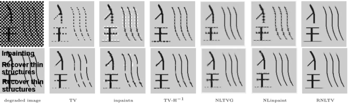
In many systems, the observed image can result from the convolution of the true image and the point spread function (PSF) contaminated by noise from various sources. The goal of

The statistics major index and inversion number, usually defined on ordinary words, have their counterparts in signed words, namely the so- called flag-major index and

The CCITT V.22 standard defines synchronous opera- tion at 600 and 1200 bit/so The Bell 212A standard defines synchronous operation only at 1200 bit/so Operation

In the first part, by combining Bochner’s formula and a smooth maximum principle argument, Kr¨ oger in [15] obtained a comparison theorem for the gradient of the eigenfunctions,

blurred cotton image and 4 kinds of algorithm recovery image after contour extraction The results of computing time on cotton images that computing time of four algorithms

the one developed in [2, 3, 1] uses R -filtrations to interpret the arithmetic volume function as the integral of certain level function on the geometric Okounkov body of the

As a final comment, we emphasize that simplicial LS-category is a new strong homotopy invariant, defined in purely combinatorial terms, that generalizes to arbitrary

The work presented here addresses an easier problem: it proposes an algorithm that computes a binary function that is supposed to capture re- gions in input space where the