Comprehensive analysis of metabolic pathways through the combined use of multiple isotopic tracers

Comprehensive Analysis of Metabolic Pathways Through the

Combined Use of Multiple Isotopic Tracers

by

Maciek Robert Antoniewicz

Master of Science in Chemical Engineering, 2000 Technical University Delft, The Netherlands

Submitted to the Department of Chemical Engineering in Partial Fulfillment of the Requirements for the Degree of

DOCTOR OF PHYLOSOPHY in Chemical Engineering

at the

MASSACHUSETTS INSTITUTE OF TECHNOLOGY June 2006

C Massachusetts Institute of Technology 2006. All rights reserved

Author

Department of Chemical Engineering May 19, 2006

- / I

77< 7

i7

r*7.

,r

Gregory Stephanopoulos Professor of Chemical Engineering Thesis Supervisor Accepted by

William M. Deen Professor of Chemical Engineering

MAsSACH~i ?s N OFTECINOLOGy

NOV .2 2006

LIBRARIES

AMtnHIVE

--Comprehensive Analysis of Metabolic Pathways Through the

Combined Use of Multiple Isotopic Tracers

by

Maciek Robert Antoniewicz

Submitted to the Department of Chemical Engineering on May 19, 2006 in partial fulfillment of the requirements for the Degree of Doctor of Philosophy

in Chemical Engineering

ABSTRACT

Metabolic Flux Analysis (MFA) has emerged as a tool of great significance for metabolic engineering and the analysis of human metabolic diseases. An important limitation of MFA, as carried out via stable isotope labeling and GC/MS measurements, is the large number of isotopomer equations that need to be solved. This restriction reduces the ability of MFA to fully utilize the power of multiple isotopic tracers in elucidating the physiology of complex biological networks. Here, we present a novel framework for modeling isotopic distributions that significantly reduces the number of system variables without any loss of information. The elementary metabolite units (EMU) framework is based on a highly efficient

decomposition algorithm identifies the minimum amount of information needed to simulate isotopic labeling within a reaction network using knowledge of atomic transitions occurring in the network reactions. The developed computational and experimental methodologies were applied to two biological systems of major industrial and medical significance.

First, we describe the analysis of metabolic fluxes in E. coli in a fed-batch fermentation for overproduction of 1,3-propanediol (PDO). A dynamic 13C-labeling experiment was

performed and nonstationary intracellular fluxes (with confidence intervals) were determined by fitting labeling patterns of 191 cellular amino acids and 8 external fluxes to a detailed network model of E. coli. We established for the first time detailed time profiles of in vivo fluxes. Flux results confirmed the genotype of the organism and provided further insight into the physiology of PDO overproduction in E. coli.

overdetermined data set we estimated net and exchange fluxes in the gluconeogenesis pathway. We identified limitations in current methods to estimate gluconeogenesis in vivo, and developed a novel [U-13C,2H8]glycerol method that allows accurate analysis of

gluconeogenesis fluxes independent of the assumption of isotopic steady-state and zonation of tracers. The developed methodologies have wide implications for in vivo studies of glucose metabolism in Type II diabetes, and other metabolic diseases.

Thesis Supervisor: Gregory Stephanopoulos Title: Professor of Chemical Engineering

To ROSANNE AND

Acknowledgements

This thesis is the result of five years of research and there are many people who both directly and indirectly contributed to it. First, I would like to thank Greg Stephanopoulos for his guidance, support, and inspiration. Joanne Kelleher introduced me to the field of

mammalian physiology and our discussions regarding limitations of current methods and the parallels between her world and mine was the inspiration for most of my research. I also had insightful discussions with Dr. McRae regarding algorithms and software, and I am grateful for his advice. I very much enjoyed the collaboration with Dave Kraynie, who turned out to be a master at crashing my software. As a result, Metran is a much better product than it would have been without his feedback. I'm also grateful for my collaboration with Jose Aleman, who performed all of the cultured hepatocyte experiments detailed in this thesis.

I have learned a lot from Sef Heijnen, Walter van Gulik, and Wouter van Winden in the past. Thank you for your mentorship. The Gregstep group members (past and present) have made my stay at MIT enjoyable and scientifically stimulating. I have collaborated closely with Adrian, Hyuntae and Matt. Adrian has been a great friend for many years. I would also like to thank my friends back in Holland -- Bart, Ton, Rob, Michiel, whom I haven't seen as much as I would have liked these last years, but I am still glad that I can count on you guys for a sanity check. I am very grateful to my parents for giving me the inspiration to work hard and never give up, and for always being there for me when 1 needed them. And thanks also to my brother, Darek, for keeping my car alive. And finally, I cannot imagine having gone through this without my intelligent and beautiful wife Rosanne. Your love, friendship, and honesty give me the strength to be a better person and to follow my dreams. I love you.

Maciek Antoniewicz May 2006

Table of Contents

Cover page

1

Abstract

3

Acknowledgments

7

Table of Contents

9

List of Figures

17

List of Tables

19

1 Introduction

23

1.1 Metabolic network and flux analysis ... ...

... 23

1.2 M etabolite flux balancing... ... 24

1.3 Estimating fluxes from stable isotope measurements...

...

25

1.4 Previous w ork ...

27

1.4.1 Isotopom ers ... 27

1.4.2 Fractional enrichm ents... ... 29

1.4.3 N M R fine spectra ... ... 30

1.4.4 M ass isotopom ers ... ... 31

1.4.5 C um om ers ... 31

1.5 Simulating labeling distributions by isotopomer balancing...

33

2.1 Introduction ... ... 39

2.1.1 M etabolic flux analysis ... 39

2.1.2 Limitations of isotopomer modeling method ... 40

2.1.3 Alternative modeling methods... 41

2.1.4 A novel framework for modeling isotopic tracer systems ... 42

2.2 T heory ... 42

2.2.1 Elementary Metabolite Units (EMU) ... ... 42

2.2.2 E M U reactions ... 43

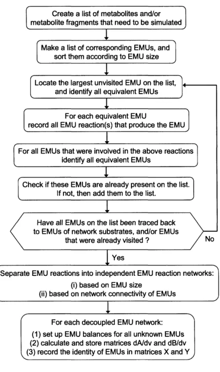
2.2.3 Decomposing metabolic networks into EMU reactions ... 46

2.2.4 Setting up EMU balances and simulating labeling distribution... 53

2.2.5 Calculating first order derivatives of simulated measurements ... 57

2.2.6 Global stability and computation time of EMU simulations ... 59

2.2.7 Identifying equivalent EMUs of metabolites... 61

2.2.8 Simulating NMR measurements using EMUs ... 70

2.3 Practical applications... 73

2.3.1 Sim ple netw ork m odel ... 73

2.3.2 T ricarboxylic acid cycle ... 74

2.3.3 Reducing EMU balances...80

2.3.4 Central carbon metabolism of E. coli... ... 82

2.3.5 Gluconeogenesis pathway ... ... ... 86

3 Determination of fluxes and confidence intervals from stable isotope measurements 91 3.1 In trod u ction ...91

3.2 Methods ... 93

3.2.1 Flux estim ation ... 93

3.2.3 Local linearized statistical properties ... 98

3.2.4 Calculating accurate flux confidence intervals ... 99

3.2.5 Relative importance of measurements ... 102

3.3 R esults ... ... 105

3.3.1 Sim ple exam ple netw ork... 105

3.3.2 G rid search... . ... 107

3.3.3 M onte Carlo sim ulations... .. 108

3.3.4 Linearized statistics ... ... 111

3.3.5 Comparison of methods for calculating flux confidence intervals ... 111

3.3.6 Mammalian gluconeogenesis... 113

3.4 D iscussion ... ... ... ... 121

A Numerically stable matrix inverse using singular value decomposition ... 123

B Algorithm for covariance-weighted flux estimation... 124

C Controlling the step size for determination of accurate flux intervals... 125

D Algorithm for accurate determination of confidence intervals of fluxes... 127

E Metabolic model of mammalian glucose metabolism... 129

4 GC/MS analysis of amino acids 131 4.1 Introduction ... ... ... 131

4.1.1 Flux analysis requires accurate data... ... 131

4.1.2 Potential sources of error ... 132

4.1.3 Reported accuracy and precision in literature ... 132

4.2 M aterials and m ethods ... ... ... 133

4.2.1 Labeled amino acid standards ... ... 133

4.2.2 Cellular am ino acids... ... 133

4.2.3 TBDMS derivatization ... 134

4.2.4 G C/M S A nalysis ... ... ... 134

4.3.2 Gas chromatography of TBDMS derivatized amino acids 135

4.3.3 Integration of mass chromatograms ... 139

4.3.4 Concentration dependence of mass isotopomer distributions ... 140

4.3.5 Validating identity of ion fragments using 13C-standards ... 145

4.3.6 Validating accuracy of mass isotopomer distributions ... 147

5 GC/MS analysis of glucose 153 5.1 Introduction ... 153

5.2 Materials and methods ... 155

5.2.1 M aterials ... 155

5.2.2 Hepatocyte isolation and cell culture ... 155

5.2.3 Preparation of experimental samples for glucose derivatization... 156

5.2.4 GC/MS analysis ... 156

5.2.5 Preparation of glucose esters ... 157

5.2.6 Preparation of aldonitrile esters of glucose ... 157

5.2.7 Preparation of methyloxime esters of glucose ... 157

5.2.8 Preparation of di-O-isopropylidene esters of glucose ... 157

5.2.9 Preparation of permethyl and perethyl derivatives of glucose ... 158

5.2.10 Data analysis ... 158

5.3 R esults .... ... 160

5.3.1 Synthesis and evaluation of glucose derivates ... 160

5.3.2 Determining deuterium labeling of glucose standards... 166

5.3.3 Study of gluconeogenesis... 172

6 Nonstationary metabolic flux analysis of E. coli 179

6.1 Introduction ... ... 179

6.2 Materials and methods ... 181

6.2.1 Stable isotope tracers ... ... ... 181

6.2.2 M edium ... . ... 181

6.2.3 Strain and growth conditions ... ... 181

6.2.4 O ff-gas analysis ... . ... 183

6.2.5 Sampling and sample processing ... 183

6.2.6 Biomass concentration ... 183

6.2.7 H PLC analysis ... ... 183

6.2.8 G C/M S analysis ... .. ... 184

6.2.9 GC/MS analysis of cellular amino acids ... 184

6.2.10 GC/MS analysis of glucose ... . ... 187

6.2.11 Calculating external fluxes ... 188

6.2.12 Metabolic network model ... 188

6.2.13 Flux determination and statistical analysis ... 189

6.3 R esults ... ... ... 189

6.3.1 E xternal fluxes ... ... 189

6.3.2 Characterization of glucose feed ... ... 192

6.3.3 Dynamics of glucose labeling... 192

6.3.4 Dynamics of fed-batch fermentation... 195

6.3.5 Nonstationary model for fed-batch fermentation ... 197

6.3.6 Metabolic flux analysis ... 199

6.3.7 Evaluation of estimated D and G parameters... 209

6.4 D iscussion ... ... ... 212

A Metabolic network model of E. coli ... ... 213

B Validation of carbon balance and degree of reduction balance... 217

C Fermentation data ... ... ... 218

D O ff-gas analysis data... 219

7.1 Introduction ... 221

7.2 M ethods ... ... 222

7.2.1 Metabolic network model ... 222

7.2.2 Estimating gluconeogenesis fluxes using MIDA ... 227

7.2.3 Simulating isotopomer distributions for '3C and 2H tracer experiments... 228

7.2.4 Analysis of a single tracer experiment ... 229

7.2.5 Simultaneous analysis of multiple tracer experiments ... ... 230

7.2.6 Statistical analysis ... ... 232

7.2.7 M aterials ... 232

7.2.8 Hepatocyte isolation and cell culture ... 233

7.2.9 Derivatization of glucose ... 233

7.2.10 GC/MS analysis ... 234

7.2.11 Measurement of metabolite concentrations ... 235

7.3 R esults ... ... 235

7.3.1 External fluxes ... .... 235

7.3.2 Reproducibility of cell experiments ... .... .... 237

7.3.3 Characterization of glycerol... 237

7.3.4 Incorporation of deuterium into lactate and ketone bodies ... 241

7.3.5 Incorporation of 13C and 2H into glucose... ... 241

7.3.6 Flux estimation and model validation... 247

7.3.7 Evaluation of estim ated fluxes ... ... ... 252

7.3.8 Comparing estimated fluxes vs. MIDA... ... 252

7.3.9 Sources of NADH ... 254

8 Application of elementary metabolite units and [U-

C,

Hjglycerol to

estimate fluxes of gluconeogenesis

259

8.1 Introduction ...

...

... 259

8.2 M ethods ... ... ... ... 261

8.2.1 M etabolic network model ... ... .. 261

8.2.2 Simulating isotopomer distributions using elementary metabolite units... 261

8.2.3 Computational methods ... ... 262

8.2.4 Determining deuterium enrichment of glucose ... 262

8.2.5 M aterials ... . ... ... ... 263

8.2.6 Hepatocyte isolation and hepatocyte suspension experiments... 263

8.2.7 Derivatization of glucose ... 264

8.2.8 GC/MS analysis ... 265

8.3 R esults ... 266

8.3.1 Incorporation of deuterium into glucose from 2H20 ... 266

8.3.2 Incorporation of labeling into glucose from [U-13C,2H8]glycerol ... 272

8.3.2 Labeling incorporation into glucose from [U-13C,2Hs]glycerol and 2H20 .... 276

8.3.3 Flux estimation and model validation ... 279

8.3.4 Evaluation of fluxes in the gluconeogenesis pathway... 279

8.3.5 Estimation of fluxes using extended model ... 281

8.4 D iscussion ... ... ... ... 285

References

287

Appendix A: GC/MS analysis of TBDMS derivatized amino acids 295

List of Figures

1-1 A schematic of metabolic flux estimation from tracer experiments ... 26

1-2 Isotopomers of a 3-atom molecule ... ... 28

1-3 Fractional enrichments are linear functions of isotopomer fractions ... 29

1-4 Mass isotopomer abundances are linear functions of isotopomer fractions ... 31

1-5 Simple metabolic network used as example for generating isotopomer balances... 34

2-1 Definition of elementary metabolite units (EMU) ... ... 44

2-2 Three types of biochemical reactions and the corresponding EMU reactions ... 45

2-3 Simple metabolic network used to illustrate EMU decomposition ... 47

2-4 Schematic overview of the algorithm for EMU decomposition ... 52

2-5 Independent EMU reaction networks generated for metabolite F ... 54

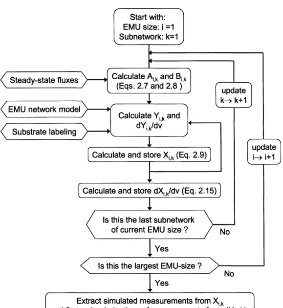
2-6 A schematic of the algorithm for simulating labeling distributions using EMUs ... 60

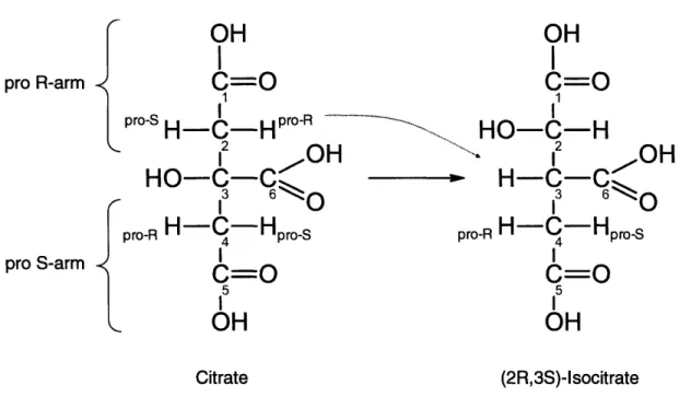
2-7 Stereospecific atom transitions for the reaction catalyzed by aconitese ... 62

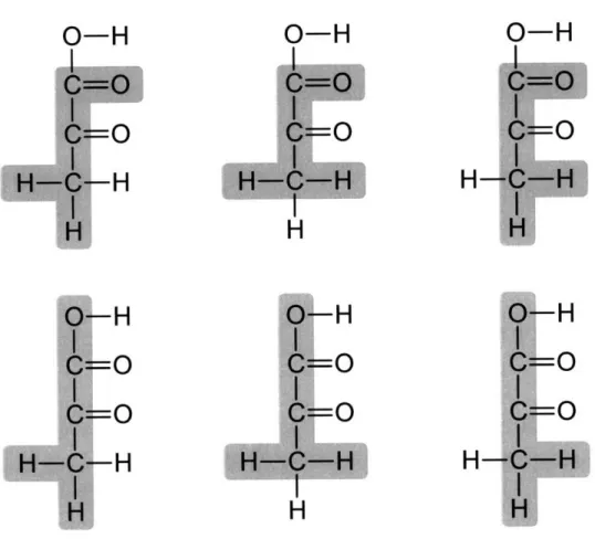
2-8 Equivalent EMUs of pyruvate ... ... 64

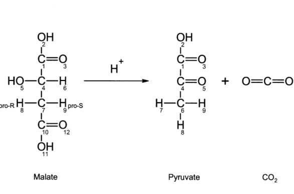
2-9 Malic enzyme converts malate to pyruvate ... 65

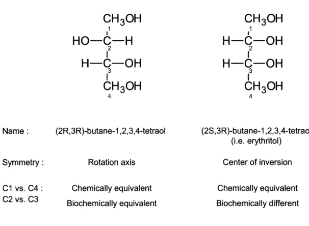
2-10 Differences between molecules with a rotation axis and center of inversion... 67

2-11 Equivalent EMUs of the rotationally symmetric fumarate ... . 69

2-12 Simplified model of the tricarboxylic acid cycle ... 76

2-13 EMU reaction networks generated for glutamate from EMU decomposition... 78

2-14 EMU balances for the EMU networks of TCA cycle... 79

2-15 Simplified EMU reaction networks for glutamate... 81

2-16 Reactions of the gluconeogenesis pathway ... ... 87

3-1 Simple metabolic network used for computation of confidence intervals ... 106

4-1

4-2 Representative total ion chromatogram from GC/MS analysis of amino acids... 137

4-3 Comparison of three methods for integration of mass chromatograms ... 141

4-4 Concentration dependence of mass isotopomer abundances ... 143

4-5 Electron ionization mass spectra of TBDMS derivatized alanine ... 146

5-1 Schematic of the two step procedure for generating glucose derivatives ... 161

5-2 Positional information obtained from the selected glucose fragments ... 163

5-3 Electron impact mass spectra of the selected glucose derivatives ... 164

6-1 A schematic of fed-batch fermentation setup and measurement points ... 182

6-2 Representative total ion chromatogram of cellular amino acids ... 185

6-3 Characterization of external fluxes in the fed-batch culture ... 190

6-4 Measured isotopic composition of glucose in the medium as a function of time... 193

6-5 Time profiles of isotopic enrichment of four intermediate metabolite pools in the pathway from glucose to biomass ... 196

6-6 Two parameter model for modeling nonstationary tracer experiments ... 198

6-7 Evaluation of goodness-of-fit for models with and without D and G-parameters ... 201

6-8 Metabolic fluxes of E. coli grown in carbon-limited fed-batch culture ... 204

6-9 Time profiles of selected intracellular fluxes ... 206

6-10 Time profiles of estimated and predicted D and G parameters...211

7-1 Reactions of the gluconeogenesis network model used for flux calculations ... 224

7-2 Algorithm for flux determination from analysis of multiple tracer experiments... 231

7-3 Time profiles of glucose, glycerol, lactate and glutamine in hepatocytes cultures ... 236

7-4 Mass isotopomer distributions of glycerol in the medium... 239

7-5 Loss of 2H from [2H5]glycerol in cultured hepatocytes ... 240

7-6 Deuterium incorporation into lactate and 3-hydroxybutyrate ... 242

8-1 Reactions involved in hydrogen exchange and hydrogen incorporation into glucose in the gluconeogenesis pathway... 271

List of Tables

2-1 EMU reactions corresponding to the three reactions in Figure 2-2 ... 46

2-2 Stoichiometry and atom transformations in the example metabolic network ... 48

2-3 Complete list of EMU reactions generated for metabolite F ... 50

2-4 Complete list of EMUs generated for metabolite F... ... 51

2-5 Comparison of three modeling approaches for simulating isotopomer labeling... 75

2-6 Stoichiometry and atom transformations for the reactions of the TCA cycle... 77

2-7 Comparison of modeling approaches for simulating mass isotopomer labeling... 83

2-8 Ion fragments of amino acids simulated using the EMU framework ... 84

2-9 Comparison of modeling approaches to simulate the labeling amino acid fragments in the E .coli network m odel ... ... ... 85

2-10 Metabolites in the gluconeogenesis pathway... ... 88

2-11 Complete list of EMUs generated for glucose from EMU decomposition of the gluconeogenesis pathway ... ... ... 89

2-12 Comparison of modeling approaches for simulating glucose labeling in the gluconeogenesis pathway... ... 90

3-1 Stoichiometry and atom transformations for reactions in the example network... 107

3-2 Comparison of methods for the calculation of confidence intervals of fluxes... 112

3-3 Stoichiometry and carbon transformations for the reactions in the network of m am m alian glucose m etabolism ... ... ... 115

3-4 Measured and fitted mass isotopomer abundances ... 117

3-5 Estimated glucose metabolic fluxes and their 95% confidence intervals ... 118

4-1 Gas chromatography retention times and main ion fragments of TBDMS derivatized amino acids ... 138

4-4 Overview of accepted amino acid fragments ... 150

4-5 Overview of rejected amino acid fragments ... 151

5-1 Overview of 18 derivatives of glucose that were synthesized and analyzed by electron impact GC/MS ... 162

5-2 Evaluation of accuracy of selected glucose fragments ... 165

5-3 Mass isotopomer distributions of selected ion fragments from glucose standards ... 167

5-4 Estimated deuterium enrichments of glucose standards ... 169

5-5 Mass isotopomer distributions of mixtures of glucose standards ... 170

5-6 Estimated deuterium enrichments of mixtures of glucose standards... 171

5-7 Mass isotopomer distributions of experimental samples ... 174

5-8 Estimated deuterium enrichments of experimental samples ... 175

5-9 Comparison of previously estimated fluxes and fluxes determined from deuterium incorporation ... 176

6-1 Ion fragment of TBDMS derivatized amino acids used for flux analysis... 186

6-2 Measured and fitted mass isotopomer abundances ... 202

7-1 Stoichiometry and atom transitions for reactions of gluconeogenesis network... 225

7-2 Assessment of biological variability in cell culture experiments ... 238

7-3 Incorporation of labeling from [13C]glycerol, [2H]glycerol and 2H20 into glucose .... 243

7-4 Corrected mass isotopomer distributions of glucose fragments ... 244

7-5 Metabolic fluxes estimated by mass isotopomer distribution analysis (MIDA) ... 246

7-6 Comparison of information content of experimental data ... 249

7-7 Estimated 95% confidence intervals of fluxes for the samples taken at 2 hr ... 251

7-8 Metabolic fluxes in the gluconeogenesis pathway estimated by combined analysis of m ultiple tracer data ... 253

7-9 Predicted fractional contribution of glycerol, water, and unlabeled sources to NADH hydrogen atoms ... 254

8-1 Mass isotopomer distributions of glucose fragments from 2_H

20 experiments with

isolated hepatocytes from fasted mice ... ... 267

8-2 Mass isotopomer distributions of glucose fragments from 2H20 experiments with isolated hepatocytes from fed mice... 268

8-3 Deuterium enrichment of glucose from 2H20 experiments with hepatocytes isolated from fasted and fed mice ... ... 269

8-4 Mass isotopomer distributions of glucose from [UI-13C,2H8]glycerol labeling experiments with isolated hepatocytes from fasted mice ... 273

8-5 Mass isotopomer distributions of glucose from [U-13C,2H8]glycerol labeling experiments with isolated hepatocytes from fed mice ... 274

8-6 Mass isotopomer distributions of glucose from [U-13C,2H8]glycerol + 2H20 labeling experiments with isolated hepatocytes from fasted mice ... 277

8-7 Mass isotopomer distributions of glucose from [U-13_C,2_{Hs]glycerol +} 2 H20 labeling experiments with isolated hepatocytes from fed mice ... 278

8-8 Comparison of information content of isotopomer data... 280

8-9 Metabolic fluxes estimated from labeling experiments... 282

Chapter 1

Introduction

1.1

Metabolic network and flux analysis

Metabolic fluxes of pathways provide a key to quantifying physiology in fields ranging from metabolic engineering to the analysis of human metabolic diseases. Understanding the regulation of cellular processes and intervening in these processes affords insight into treating disease and achieving other biotechnological objectives. Living cells are complex biological entities that are regulated at many levels, e.g. transcription, translation, protein

modification, etc. A large number of reactions, comprising a well-organized system of enzymatic activities, accomplish the conversion of relatively simple molecules such as glucose into a wide variety of small- and macromolecules. The conversion of each individual

reaction may be overseen easily, however, the result of the overall system of reactions is often not trivial. Identification of targets for pathway manipulation and determining the required magnitude of biological changes requires an enhanced, quantitative understanding of cellular metabolism and regulation. Metabolic flux analysis (MFA) has emerged as an important tool to assess the metabolic state of living cells and to evaluate the effects of genetic and environmental manipulations. Fluxes of metabolic pathways are considered fundamental determinants of cell physiology and informative parameters in evaluating cellular mechanisms, regulation and causes of disease. The key to quantifying metabolic

fluxes is to analyze biological systems as integrated and interacting networks, rather than a set of individual components.

1.2

Metabolite flux balancing

Tools for estimating metabolic fluxes are fundamentally different from the tools for

obtaining static measurements such as metabolite concentration and transcript levels, which

provide relatively little insight into the dynamics of cellular metabolism. Initially, metabolic flux analysis relied solely on balancing fluxes around metabolites within an assumed network stoichiometry. Assuming metabolic steady-state, fluxes (v) are constrained by the

stoichiometry matrix (S).

S-v

=

0

(1.1)

Stoichiometric constraints can be combined with the flux measurements matrix (R) that contains a row with a unity entry for each measured external flux. The combined

stoichiometry and measurement matrices are then used to obtain the generalized solution to the metabolite flux balancing problem by solving a set of linear equations. The solution to this problem is given by the following expression:

v =

.

null

P

(1.2)

Here, 'pinv' denotes the pseudo inverse, and 'null' is the null space of the combined stoichiometry and measurement matrix. Vector 0 contains the linear coefficients of the columns that span the null space. In most practical situations, however, stoichiometric constraints and external flux measurements did not provide enough information to estimate all fluxes of interest in complex biological systems with reversible reactions, parallel

pathways and internal cycles. This limitation let to the development of isotopic tracer techniques to determine fluxes.

CHAPTER 1. INTRODUCTION

1.3

Estimating fluxes from stable isotope measurements

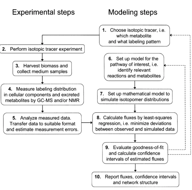
A more powerful method for flux determination in complex biological systems is based on the use of stable isotopes. Figure 1-1 shows schematically the procedure for quantifying metabolic fluxes from stable isotope experiments. The first two important decisions are the choice of the isotopic tracer and the structure of the metabolic network model (steps 1 and 6). Methods for experiment design are aimed at finding the most informative tracer(s) for a given set of stable isotope measurements using criteria from linearized statistics and

sensitivity analysis (Mollney et al., 1999). Metabolic flux studies further require some prior knowledge of the biochemical reactions involved in the pathway of interest. The decision which reactions and metabolites to include in the network model is still mainly driven by the investigators' insight into the physiology and may in some cases be somewhat arbitrary. However, we will illustrate in Chapter 3 that proper statistical analysis of isotopomer data

can be instrumental in identifying the most likely network structure. Steps 2-4 are

experimental in nature and require good laboratory skills. In labeling experiments, metabolic conversion of isotopically labeled substrates generates molecules with distinct labeling patterns (i.e. isotopomers) that can be detected by mass spectrometry (MS) and nuclear magnetic resonance (NMR) spectroscopy (Szyperski, 1995; Des Rosiers, 2004) (step 4). In general, the NMR technique requires expensive equipment and a fairly large amount of

sample, which limits the use of this technique to a few expert groups. On the other hand, GC/MS analysis is a more rapid and sensitive technique that is readily accessible to many research labs. Raw data from both techniques needs to be further processed before it can be used for flux determination. In both cases, data processing consists of the detection of metabolite peaks in NMR and MS spectra and integration of peak intensities (step 5). The isotope measurements provide many additional independent constraints for MFA.

Quantitative interpretation of the isotopomer data requires the use of large-scale mathematical models that describe the relationship between metabolic fluxes and

isotopomer abundances (step 7). Schmidt developed an elegant method for automatically generating the complete set of isotopomer balances for any given network using a matrix based method (Schmidt et al., 1997), and more recently Wiechert et al. (1999) provided an

Experimental steps

Modeling steps

{1.

Choose isotopic tracer, i.e.

which metabolite

and what labeling pattern

Perform isotopic tracer experiment

3. Harvest biomassand

collect medium samples

4. Measure labeling distribution

in cellular components and excreted

metabolites by

GC-MS

and/or NMR

5. Analyze measured data.

Transfer data to suitable format

and estimate measurement errors.

`r

6. Set up model for the

pathway of interest, i.e.

identify relevant

reactions and metabolites

7. Set up mathematical moc

simulate isotopomer distribut

8. Calculate fluxes by least-sq

regression, i.e. minimize devi•

between observed and simulate

lelto

ions

uares

ati'

ons

data

9. Evaluate goodness-of-fit

and calculate confidence

intervals of estimated fluxes

10.

Report fluxes, confidence intervals

and network structure

Figure 1-1: A schematic of metabolic flux estimation from tracer experiments. Metabolic flux analysis is characterized by both experimental and analytical steps. The dotted lines indicate that MFA is an iterative process that requires reevaluation of metabolic network assumptions and the choice of optimal tracer.

2.

CHAPTER 1. INTRODUCTION

In the forward calculation, these isotopomer models simulate a unique profile of isotopomer abundances for given steady-state fluxes. In MFA we solve the more challenging inverse problem, i.e. determining the cell's flux state from measurements of isotopomer

distributions. Analytical solutions to this inverse problem are only available for very simple systems. Therefore, fluxes in complex biological systems have to be determined by iterative least-squares fitting procedures, where the objective is to evaluate a set of feasible fluxes that best accounts for the observed isotopomer measurements (step 8). At convergence, the goodness-of-fit is evaluated using statistical criteria and confidence intervals of fluxes are determined (step 9). The final result of this whole process is a detailed flux map (with confidence intervals) that describes the contribution of various metabolic reaction pathways to the overall cellular metabolism. The dotted lines in Figure 1-1 illustrate that metabolic flux analysis is an iterative process that requires constant reevaluation of metabolic network assumptions and the choice of optimal tracer.

1.4

Previous work

A range of stable isotopes such as 13C, 2H, 15N, and 180 can be used to trace metabolic pathways using GC/MS and NMR measurements. Currently, methods based on carbon-13 tracing are most widely used. In this section we provide a short review of the most important concepts currently used in metabolic tracer analysis, i.e. isotopomers, fractional enrichments, NMR fine spectra, mass isotopomers, and cumomers.

1.4.1

Isotopomers

Positional isotopomers (or simply isotopomers) are isomers of a metabolite that differ only in the labeling state of their individual atoms, for example, 13C VS. 12C in carbon-labeling studies, and 2H vs. 1H in hydrogen-labeling studies. For a metabolite comprising N atoms that may be in one of two (labeled or unlabeled) states, 2" isotopomers are possible. Thus, a molecule consisting of 3 atoms can exist in 8 specific labeling states (see Figure 1-2). We can represent the labeling patterns of isotopomers as sequences of ones and zeros that can be

The isotopomer distribution vector (IDV) contains the molar fractions of the 2N isotopomers. For example, the first element in the IDV contains the molfraction of the isotopomer with labeling pattern 000, i.e. unlabeled molecule. The second element corresponds to labeling pattern 001, i.e. molecule with a single labeled atom at the third position, and so forth. Note that by definition, the sum of all elements of IDV equals one. In practice, isotopomer fractions are not measured directly. Instead, available measurements are

expressed as functions of isotopomer fractions. The two most widely used techniques for measuring labeling distribution are nuclear magnetic resonance (NMR) spectroscopy and mass spectrometry (MS), which are discussed next.

Isotopomers

000

060

OS

amO

Figure 1-2: Isotopomers of a 3-atom molecule. The 8 (=23) isotopomers are shown on the left. The spheres represent labeled (full) and unlabeled (open) atoms. The isotopomer distribution vector (IDV) contains the molfractions of all isotopomers. By definition, the

sum of all isotopomer fractions equals one.

CHAPTER 1. INTRODUCTION

1.4.2

Fractional enrichments

The NMR technique detects magnetic interaction between 13C-nuclei and adjacent nuclei with magnetic spins, e.g. 1H and adjacent 13C nuclei. NMR analysis provides two types of labeling information. First, one can determine the fractional abundance of 13C at a specific

carbon atom position, which is called the fractional enrichment (FE) measurement. Determination of fractional enrichments is based on the fact that the 1H-'2C interaction gives rise to a different peak in the 1H-NMR spectrum than the 1H-13C interaction.

Fractional enrichments of individual carbon atoms can be interpreted as linear functions of isotopomer fractions. For example, consider the fractional enrichment of the first atom of the 3-atom molecule A, i.e. A#1, which is simply the sum of the four isotopomer fractions

for which the first atom is labeled (i.e. A1oo, Ao10 , Allo0, and A111). Figure 1-3 shows the linear

relationship between fractional enrichments and isotopomer fractions. Note that the term fractional enrichment is somewhat misleading, i.e. one doesn't actually measure the enrichment of 13C. The term 'positional abundance of t3C' would have been more appropriate.

Fractional enrichments

O)O

06OO

8

Oft

4+

1.4.3 NMR fime spectra

Adjacent 13C-13C nuclei influence each others NMR signal by peak splitting (a phenomenon called J-coupling), which is observed in the 13C-NMR spectrum. Peak splitting leads to the formation of multiple fine structures in the NMR spectrum, e.g. singlets, doublets, triplets, doublets of doublets, etc. The relative contribution of individual multiplets to the resulting overall multiplet pattern provides not only information on the labeling state of individual carbon atoms of a molecule, but also detailed positional information. For example, consider a molecule consisting of 2 carbon atoms. The 13C-multiplet peak areas can be expressed as a nonlinear function of three isotopomer fractions. Eq. 1.3 converts 13C-multiplet peak areas to relative areas, in this case two singlets and a doublet in the 13C-NMR spectrum.

singlet 2

A

A,

Eq. 1.4 shows the relationships for a secondary carbon atom, where we also take into account long range 13C-13C interactions.

singlet 2 doublet 24 doublet 23 double doublet 234 doublet 12 double doublet 124 double doublet 123 quadruple doublet 1234 A0101 A010

A111c

S(A,,oo + A01l +A,,010 + A,0 +A 11 11,,, 1+A +A1+110 +A1111

CHAPTER 1. INTRODUCTION

1.4.4 Mass isotopomers

Mass spectrometry (MS) is an analytical technique where molecules are separated according to their mass to electric charge ratio, i.e. m/z ratio. Isotopomers that have incorporated the same number of labeled atoms, called mass isotopomers, contribute to the intensity of the same ion peak in a mass spectrum. Mass isotopomer distribution reflects the relative amounts of each mass isotopomer (including the unlabeled fraction). Mass isotopomer distribution (MID) can be interpreted as a linear mapping of isotopomer fractions, as is illustrated in Figure 1-4. Note that the sum of the mass isotopomer distribution vector is by definition one.

Mass isotopomers

Ai,)l

Amo Am-, _AM+2 AM3 A+ ' 1 0 0 0 0 O A100

000 0

A M+₂ 0 0 1 0 1 1 0 A,)_O

A

0 0

0 0

0

0 1

A

S00066

A,,

Figure 1-4: Mass isotopomer abundances are linear functions of isotopomer fractions. By definition the sum of all mass isotopomer fractions is one.

1.4.5 Cumomers

Wiechert et. al. (1999) introduced the concept of cumomers, i.e. short for cumulative isotopomers, as a method to simplify isotopomer simulations (see section 1.6). In essence, cumomers are simply a linear mapping of isotopomers. For example, consider a 3-atom

molecule A. The so called 0-cumomer fraction is the sum of all isotopomer fractions, and is

(1.4)

1

Ax

=

i,j,k=0

Here, subscript 'x' has the meaning '0 or 1'. Using the same convention, the 1-cumomer

fractions are defined as follows:

1 AIXX= -Alik , j,k=0 1 A x

=,

(1.5)

Thus, the 1-cumomer fractions are sums of those isotopomer fractions that are labeled at least at the position indicated by the index 1. By this definition, 1-cumomer fractions are identical to fractional enrichments, i.e. A#1 =Ai, A#2=Ax,x, and A#3=Axx1. Following the

same convention, the 2-cumomer fractions are sums of those isotopomer fractions where at least two of the three atoms are labeled indicated by the index 1:

Al x = Allk , k=O 1 AIx, = EAl, i=0 (1.6) AXl, = Ai1M i=o

Finally, the 3-cumomer fraction A11 corresponds to the fully labeled isotopomer fraction All1.

A I -- AllI (1.7)

Wiechert showed that there is always a linear one-to-one relationship between cumomer and isotopomer fractions. For an N atom molecule, the transformation from its 2-N isotopomer

fractions to the corresponding 2N cumomer fractions is given by the transformation matrix T, which is constructed recursively in the following manner.

(1.8)

CHAPTER 1. INTRODUCTION

Thus, for a 3-atom molecule fractions is given by Eq. 1.9.

A _aXXxx Alx, Axl Axx AlxX All _

the transformation from isotopomer fractions to cumomer

A000 A₀₀₁ A₀₁₀ A₀₁₁ A101 A110 All _Alll (1.9)

The reverse transformation, i.e. from cumomer fractions to isotopomer fractions, is achieved by inverting the transformation matrix. Wiechert showed that the transformation matrix of any size is always full rank, i.e. invertible.

1.5

Simulating labeling distributions by isotopomer balancing

Here, we describe the method that is currently used for simulating labeling distributions in reaction networks. This method was originally based isotopomer balancing, but has been replaced more recently by cumomer balancing. Consider the simple network model shown in Figure 1-5 that consists of 4 metabolites, 3 extracellular fluxes and 3 intracellular reactions. Here, the third reaction is considered reversible and is modeled by separate forward and backward reactions. Metabolite A is the network substrate with known labeling and metabolites C and D are the two products whose labeling pattern we would like to predict for given fluxes. Figure 1-5 (right panel) also shows the assumed atom transitions for the reactions in this network. Similar to metabolite balancing, we can set up material balances for all 12 unknown isotopomers in this system. The complete set of isotopomer balances is shown below.

---Reaction stoichiometry

A

- -

B

Atom transitions

AB---I

V

b

C

D

23

Figure 1-5: Simple metabolic network model used as example for generating isotopomer balances. Reaction stoichiometry is shown in the left panel and the assumed atom transitions are shown in the right panel.

WI

CHAPTER 1. INTRODUCTION

0 = vlyaoo + V3b'doo - (v3f+v2)-boo (1.10a)

0 = vl-aol + V3b'd01 - (v3f+v2)'bo0 (1.10b)

0 = _{vlalo + V3b'dl0 - (v3f+v2)-blo}

(1.10c) 0 = vlall + V3b'dl - (v3f+v2)-'bl (1.10d) 0 = v2-(aoo0boo + aoo-bo1 + aor-boo + ao-bol) - w2-C00 (1.10e) 0 = v2-(aoob00o + aoo-bil + aol-bio + aol-bil) - w2"CO (1.10f)

0 = v2-(aio-boo + aiobol + aiboo + allbol) - w2-C0 (1.1Og) 0 = v2-(aio-bio + a0o-bi, + al-bio + ali-bi) - w2-CI (1.10h)

0 = vl-(aoo-boo + aoo-blo + alo-boo + alo-blo) + v3fboo- (v3b+W3)-doo (1.10i) 0 = vl-(aoo-bo1 + aoo-bi1 + alo-bol + alo-bi) + v3f-bol- (V3b+W3)-do0 (1.10j) 0 = vy-(ao-boo + aoi'blo + ailboo + ali-bio) + v3f-bo- (v3b+W3)-d0o (1.10k) 0 = vl'(aol-boi + aol'bil + all-boi + aull-bi) + v3f-bi- (v3b+w3)-dul (1.101)

For given fluxes and labeling input, the isotopomer balances provide 12 nonlinear equations in 12 unknown isotopomer fractions, which can be solved using Newton's iterative method. As the result we obtain the isotopomer fractions for all 12 unknown isotopomers in this system.

1.6

Simulating labeling distributions by cumomer balancing

Wiechert et. al. (1999) recently showed that the complete set of nonlinear isotopomer balances can be converted into a corresponding set of cumomer balances. It was shown that cumomer balances are less strongly coupled then isotopomer balances, which allows

cumomer balances to be solved explicitly as a cascade of linear subproblem, from which the 1-, 2-, ... cumomer fractions are successively computed. The cumomer fractions are then transformed to isotopomer fraction as described in section 1.4.5. The major difference between cumomer and isotopomer balances is the fact that cumomer balances are always linear in the unknown variables. Thus, each subproblem can be solved using linear algebra

size of the problem is same for both methods, i.e. there are always as many cumomer balances as there are isotopomer balances.

1.7

Aim and outline of thesis

Our research group has actively participated in the development of experimental and computational methods for MFA based on stable isotope experiments. The first general mathematical model for interpreting of fractional enrichments was developed by Zupke and

Stephanopoulos (1995). In the last decade MFA has reached a state of relative maturity. The experiments themselves have become a routine procedure, measurement techniques such as GC/MS are widely used, and advanced mathematical procedures are available for

quantitative interpretation of stable isotope measurements.

The most important limitation of current methodology for MFA, as carried out via stable isotope labeling and GC-MS measurements, is the large number of isotopomer/cumomer equations that need to be solved, especially when multiple isotopic tracers are used for the labeling of the system. This reduces the ability of MFA to fully utilize the power of multiple isotopic tracers (i.e. 13C and 2H tracers) in elucidating the physiology of realistic situations comprising complex bioreaction networks. As such, the realm of tracer experiments is currently limited to carbon-13 tracers only. Therefore, the main goal of this thesis work was the development of a novel methodology for comprehensive analysis of metabolic pathways through the combined use of multiple isotopic tracers.

Chapter 2 describes the novel framework for modeling isotopic distributions that significantly reduces the number of system variables without any loss of

information. The elementary metabolite unit (EMU) framework is based on a highly efficient decomposition algorithm that identifies the minimum amount of

information needed to simulate isotopic labeling within a reaction network using the knowledge of atomic transitions occurring in the network reactions. For a typical carbon labeling system the total number of equations that needs to be solved is

CHAPTER 1. INTRODUCTION

reduced by one order-of-magnitude (100s EMUs vs. 1000s cumomers). As such, the EMU framework is most efficient for the analysis of labeling by multiple isotopic tracers. For example, analysis of the gluconeogenesis pathway with 2H, 13C, and 180

tracers required only 300 EMUs compared to 3,000,000 isotopomers/cumomers.

* Chapter 3 describes novel methodologies for flux determination and statistical analysis that have been developed. A serious drawback of the flux estimation method in current use is that it does not produce confidence limits for the estimated fluxes. Without this information it is difficult to interpret flux results and expand the physiological significance of flux studies. To address this shortcoming we derived analytical expressions of flux sensitivities with respect to isotope measurements and measurement errors. These tools allow determination of local statistical properties of fluxes and relative importance of measurements. Furthermore, we developed an efficient algorithm to determine accurate nonlinear confidence intervals of fluxes and demonstrated that confidence intervals obtained with this method closely approximate true flux uncertainty.

* Chapters 4 and 5 describe experimental protocols that were developed for accurate and precise measurement of labeling distributions by GC/MS. In the context of this thesis work, the main focus was on accurate measurement of mass isotopomer distributions of cellular amino acids and glucose. Based on preliminary simulations and sensitivity analysis of realistic metabolic networks we determined that errors in mass isotopomer abundances should be less than 0.5 mol%. The main result of our work is a detailed procedure for the assessment of mass isotopomer distributions of cellular amino acids and glucose with an accuracy of 0.4 mol% and precision of 0.2 mol%, or better.

* Chapter 6 describes analysis of metabolic fluxes in a nonstationary biological system of with industrial relevance, i.e. microbial fed-batch fermentation of E. coli for the overproduction of 1,3-propanediol (PDO). A drawback of current methods

and to extend the scope of flux determination from stationary to nonstationary systems we developed a novel modeling strategy that combines key ideas from isotopomer spectral analysis (ISA) and stationary MFA. In this study, metabolic fluxes were determined at multiple time points during a fed-batch culture, and as such we established for the first time detailed time profiles of intracellular fluxes in a fermentation.

Chapters 7 and 8 describe analysis of fluxes in the gluconeogenesis pathway from cultured primary hepatocyes, i.e. isolated liver cells. We applied multiple 13C-, and

2

H-labeled tracers and analyzed the resulting mass isotopomer distributions of glucose fragments. From this overdetermined data we estimated, for the first time, both net and exchange fluxes in the gluconeogenesis pathway and calculated confidence intervals for fluxes. We identified limitations in current methods to estimate gluconeogenesis fluxes in vivo, and developed a novel multiple-tracer method for accurate and quantitative analysis of this pathway independent of the isotopic steady-state assumption.

Chapter 2

Elementary Metabolite Units (EMU):

a novel framework for modeling isotopic

distributions

2.1

Introduction

2.1.1 Metabolic flux analysis

Accurate flux determination is of great importance for the analysis of cell physiology in fields ranging from metabolic engineering to the study of human metabolic diseases (Brunengraber et al., 1997; Hellerstein, 2003; Stephanopoulos, 1999). Initially, metabolic flux analysis (MFA) relied solely on balancing fluxes around metabolites within an assumed network

stoichiometry. However, stoichiometric constraints and external flux measurements often cannot provide enough information to estimate all fluxes of interest. A more powerful method for flux determination in complex biological systems is based on the use of stable isotopes (Wiechert et al., 2001). Metabolic conversion of isotopically labeled substrates generates molecules with distinct labeling patterns, i.e. isotope isomers (isotopomers), that can be detected by mass spectrometry (MS) and nuclear magnetic resonance (NMR) (Szyperski et al., 1995). Isotope measurements provide many additional independent constraints for MFA. It has been shown that at metabolic and isotopic steady state the isotopomer composition of metabolic intermediates is fully determined by the cell's flux

state and the administered isotopic label. Quantitative interpretation of isotopomer data requires the use of mathematical models that describes the relationship between metabolic fluxes and the observed isotopomer abundances. Similar to metabolite balancing, balances can be set up around all isotopomers of a particular metabolite. Schmidt described an elegant method for automatically generating the complete set of isotopomer balances using a matrix based method (Schmidt et al., 1997). More recently, Wiechert introduced the concept of

cumulative isotopomers (cumomers) and provided and efficient procedure for solving isotopomer models (Wiechert et al., 1999). In the forward calculation, isotopomer models

are used to simulate a unique profile of isotopomer abundances for given steady-state fluxes. In MFA we are concerned with the more challenging inverse problem, i.e. to determine the flux state of the cell from measurements of isotopomer distributions. Analytical solutions to the inverse problem are only available for very simple systems. Thus, in general, fluxes in complex biological systems will be determined by iterative least-squares fitting procedures.

2.1.2

Limitations of isotopomer modeling method

Isotopomers are defined as isomers of a metabolite that differ only in the labeling state of

their individual atoms, for example, 13C vs. 12C in carbon-labeling studies, and 2H vs. 1H in

hydrogen-labeling studies. For a metabolite comprising N atoms that may be in one of two

(labeled or unlabeled) states, 2N'' isotopomers are possible. Consequently, the number of isotopomers can increase quickly when multiple tracers are applied. Consider for example

glucose (C6H1206). There are only 64 (=26) carbon atom isotopomers of glucose and 4096

(=212) hydrogen atom isotopomers, but there are 2.6x105 (=26x212) isotopomers of glucose carbon and hydrogen atoms, and 1.9x108 (=26x212x36) isotopomers of glucose carbon, hydrogen and oxygen atoms. Note that oxygen may be present in one of three stable forms, i.e. 160, 170, and 180. Thus, a typical isotopomer model may contain thousands or even

millions of isotopomers for multiple isotopic tracers. The number of isotopomers may be reduced somewhat by omitting unstable carboxyl and hydroxyl hydrogen atoms from the

model, which exchange with the solvent at rates much faster than biochemical reactions and are also lost in chemical derivatization in preparation for GC/MS analysis. For example, if we consider only the seven stable (i.e. carbon bound) hydrogen atoms of glucose, then there

CHAPTER 2. ELEMENTARY METABOLITE UNITS

are 128 (=2D) hydrogen atom isotopomers, 8192 (=26x2D isotopomers of glucose carbon and hydrogen atoms, and 6x106 (=26x27x36) isotopomers of glucose carbon, hydrogen and oxygen atoms. Thus, even with this reduction there are still too many isotopomers to simulate labeling distributions efficiently for multiple isotopic tracers. Note that the cumomer method suffers from the same problem, because there are always as many cumomers as isotopomers, i.e. there is a one-to-one relationship between cumomers and isotopomers (Chapter 1). As such, the realm of tracer experiments is currently limited solely

to 13C-tracers. However, multiple isotopic tracers are more powerful in elucidating the physiology of realistic situations comprising complex bioreaction networks (see Chapters 7

and 8). Therefore, the development of a methodology that extends the capability of MFA beyond the use of a single isotopic tracer is the main goal of this work.

2.1.3 Alternative modeling methods

The isotopomer/cumomer modeling framework is a generic top-down modeling strategy. It

provides the most detailed description of the labeling state of a system given by the

isotopomer fractions of all metabolites. However, the large number of variables generated in this modeling approach limits its application and has driven the development of alternative

modeling methods for specific isotope measurements. For example, it is well know that fractional enrichments of carbon atoms can be simulated efficiently using atom mapping matrices, the method that was originally proposed by Zukpe et al. (1994). More recently, Van Winden et al. (2002) developed the concept of bondomers that allows efficient simulation of NMR fine spectra and MS data without the use of isotopomers. However, the bondomer method is only valid for 13C-labeling data from experiments where a single uniformly 13C_ labeled substrate is applied. If multiple carbon sources are present, then all substrates need to be uniformly 13C-labeled with the same enrichment. This requirement significantly limits the applicability of the bondomer method. As such, there is still no general method for simulating mass isotopomer distributions in complex biological systems that avoids the use of isotopomers/cumomers.

2.1.4 A novel framework for modeling isotopic tracer systems

Here, we present a novel framework for modeling isotopic tracer systems that significantly reduces the number of system variables without any loss of information. The elementary

metabolite units (EMU) framework is a bottom-up modeling approach that is based on a highly efficient decomposition algorithm that identifies the minimum amount of information needed to simulate isotopic labeling within a reaction network. The functional units

generated by the decomposition algorithm, called elementary metabolite units, form the new basis for generating system equations that describe the relationship between fluxes and isotopomer abundances. Isotopomer abundances simulated using the EMU framework are identical to those obtained using the isotopomer and cumomer methods, however, require significantly fewer variables. For a typical carbon labeling system the total number of

variables and equations that needs to be solved is reduced by one order-of-magnitude (100s EMUs vs. 1i000s isotopomers/cumomers). As such, the EMU framework is most efficient for the analysis of labeling by multiple isotopic tracers. For example, analysis of the

gluconeogenesis pathway probed with 2H and 13C tracers required only 145 EMUs compared to more than 4x104 isotopomers/cumomers.

2.2

Theory

2.2.1 Elementary Metabolite Units (EMU)

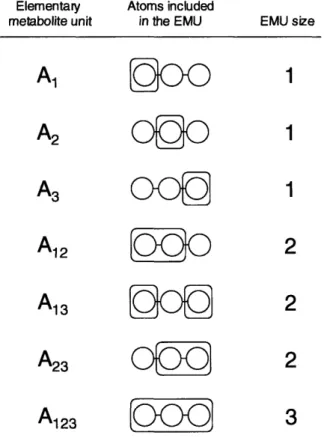
We define elementary metabolite units as distinct subsets of metabolite's atoms. For example, consider metabolite A consisting of 3 atoms. An EMU is a subset of any number of these 3 atoms. The size of an EMU is defined as the number of atoms that are included in the EMU. There are 7 possible EMUs for metabolite A: 3 EMUs of size 1 (A1, A2, A3), 3

EMUs of size 2 (A12, A13, A23), and 1 EMU of size 3 (A123), where the subscript denotes the

atoms that are included in the EMU (see Figure 2-1). Note that atoms in an EMU are not necessarily connected by chemical bonds, for example consider EMU A13. In general, for a

CHAPTER 2. ELEMENTARY METABOLITE UNITS

Theoretical maximum number of EMUs =

(2.1)

In this Chapter, we will illustrate that the EMU framework can be used for simulation of

isotopic labeling within a reaction network using the minimum number of variables, all of

which are expressed in terms of EMUs. In most cases, only a small number of all possible

EMUs is required to simulate the isotopic labeling. In the next section, we will illustrate the

EMU approach for simulating MS measurements, and in section 2.2.8 we will show how

NMR measurements can be simulated using EMUs.

2.2.2 EMU reactions

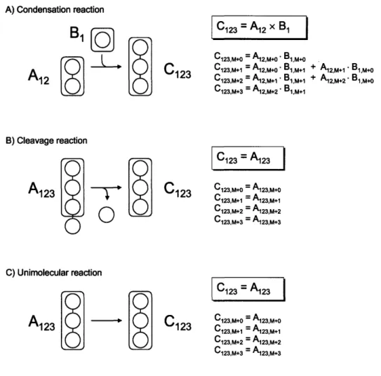
First, we need to introduce the concept of an EMU reaction. Figure 2-2 shows three types of

biochemical reactions that we can distinguish: a condensation reaction, a cleavage reaction,

and a unimolecular reaction. For each reaction type in Figure 2-2 we would like to determine

the minimum amount of information that is needed to determine the mass isotopomer

distribution (MID) of product C, i.e. EMU C123. For the condensation reaction, MID of C123

is fully determined by the MIDs of EMUs A

and B

. For example, the M+O abundance of

C123 is

equal to the product of M+0O abundances of A

and

i.e.

The full MID of C

is obtained from the convolution (or Cauchy product, denoted by 'x)

of MIDs of A12 and B1, i.e. C123=A12xB1. For the cleavage and unimolecular reactions, MID

of C123 is equal to MID of the EMU A123.Note that for the cleavage reaction atoms of A

that are not transferred to C

are not considered in the EMU reaction, i.e. their labeling

doesn't affect the labeling state of C. Note also that EMU reactions are always size balanced,

i.e. the EMU product is formed either from EMUs of the same size, or by condensation of

smaller EMUs such that the total size of substrate EMUs equals the size of the EMU

product. Thus, there can only be only two types of EMU reactions: condensation and

unimolecular EMU reactions. Table 2-1 shows the EMU reactions corresponding to the

biochemical reactions in Figure 2-2.

Elementary Atoms included

metabolite unit in the EMU EMU size

A,

O

1

A

2

Oo

1

A

1

A

KD

2

A

D

2

A

2

O____

3

Figure 2-1: Elementary metabolite units (EMU) are defined as distinct subsets of

metabolite's atoms. There are 7 EMUs for a 3-atom metabolite A. The subscript in the first column denotes the atoms that are included in the respective EMU. The EMU size is defined as the number of atoms included in the EMU.

CHAPTER 2. ELEMENTARY METABOLITE UNITS

A) Condensation reaction

A12

_A

C123

1 2

C

3

=

A

B

C₁₂₃,M+O = A12,M+0 B1,M+O

C123,M+1 = A12,M+O. B1,M+1 + A12,M+1" 1,M+O

C123,M+2 = A12,M+1 B,M+1 + A12,M+2 Bl,M+o

C123,M+3 = A12,M+2* B1,M+1 B) Cleavage reaction

A

₁₂₃

_C

₁₂₃

0

A

S

C

123

Figure 2-2: Three types of biochemical reactions and the corresponding EMU reactions. Shaded areas indicate atoms included in the EMUs. The mass isotopomer distribution (MID) of product C is fully determined by MIDs of substrate EMUs. Thus, for the condensation reaction, MID of C123 is obtained from the convolution (or Cauchy product,

denoted by 'x') of MIDs of A12 and B1. For the cleavage reaction and unimolecular reaction

Table 2-1

EMU reactions corresponding to the three reactions shown in Figure 2-2. Note that EMU reactions are always EMU size balanced, i.e. the size of the EMU product always equals the total size of substrate EMUs.

Reaction type Biochemical reaction EMU reaction EMU size balance Condensation A + B - C A12+ B1 - C123 2 + 1 = 3

Cleavage A B + C A1 23 -C 123 3

=

Unimolecular A - C A1 23 - C12 3 3 = 3

2.2.3 Decomposing metabolic networks into EMU reactions

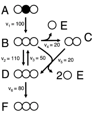
We will now describe the algorithm that systematically decomposes any biochemical reaction network into EMU reactions using the knowledge of atomic transitions occurring in the network reactions. These EMU reactions will then form the basis for generating model equations for isotopic simulations (see section 2.2.4). Consider the example network shown in Figure 2-3 that will be used to illustrate the theory behind EMU modeling. In this network, metabolite A is the sole substrate and metabolites E and F are two network products. The intermediary metabolites B, C and D are assumed to be at metabolic and isotopic steady state. The stoichiometry and atom transitions for the five reactions are given in Table 2-2, and the assumed flux distribution is shown in Figure 2-3. The structural input that is required for the EMU decomposition is threefold:

1. The assumed metabolic network stoichiometry 2. Atom transitions for all reactions in the network

CHAPTER 2. ELEMENTARY METABOLITE UNITS

A 060

V1= 100

O

_E

B

C000

(D

C

v

=

110

V

50

₅₌

= 20

D

CCO

₂₀

_E

_80j

F 000

Figure 2-3: Simple metabolic network used to illustrate the decomposition of a metabolic system into EMU reactions. The assumed steady-state fluxes have arbitrary units. The network substrate A is fully labeled on the second atom. Atom transitions for the reactions in this model are given in Table 2-2.

Table 2-2

Stoichiometry and atom transformations for reactions in the example metabolic network. This simple metabolic network is used to illustrate the decomposition of a metabolic system into EMU reactions.

Reaction Reaction stoichiometry Atom transformations* number 1 A --+ B abc --+ abc 2 B - D abc <- abc 3 B - C + E abc -> bc + a 4 B + C - D+ E + E abc + AB -- bcA + a + B 5 D -+ F abc -+ abc

* For each compound atoms are identified using lower case letters to represent successive atoms of each compound. Uppercase letters represent a second compound in the reaction.