HAL Id: hal-02342441
https://hal.archives-ouvertes.fr/hal-02342441
Submitted on 11 Jan 2020
HAL is a multi-disciplinary open access
archive for the deposit and dissemination of
sci-entific research documents, whether they are
pub-lished or not. The documents may come from
teaching and research institutions in France or
abroad, or from public or private research centers.
L’archive ouverte pluridisciplinaire HAL, est
destinée au dépôt et à la diffusion de documents
scientifiques de niveau recherche, publiés ou non,
émanant des établissements d’enseignement et de
recherche français ou étrangers, des laboratoires
publics ou privés.
Integrated Laycan and Berth Allocation Problem
Hamza Bouzekri, Gülgün Alpan, Vincent Giard
To cite this version:
Hamza Bouzekri, Gülgün Alpan, Vincent Giard. Integrated Laycan and Berth Allocation Problem.
International Conference on Industrial Engineering and Systems Management, Sep 2019, Shanghai,
China. pp.1-6, �10.1109/IESM45758.2019.8948110�. �hal-02342441�
978-1-7281-1566-5/19/$31.00 ©2019 IEEE
Integrated Laycan and Berth Allocation Problem
Hamza Bouzekri
1, 21 EMINES - School of Industrial
Management,
Mohammed VI Polytechnic University Ben Guerir, Morocco
Gülgün Alpan
1, 22 Univ. Grenoble Alpes,
Grenoble INP, CNRS, G-SCOP Grenoble, France [email protected]
Vincent Giard
1, 33 Paris Dauphine University,
PSL Research University Paris, France
Abstract—Handling vessels within the agreed time limits at a
port with an optimal exploitation of its quays plays an important role in the improvement of port effectiveness as it reduces the stay time of vessels and avoids the payment of contractual penalties to shipowners due to the overrun of laytimes. In this paper, we propose a mixed zero-one linear model for a new problem called the integrated Laycan and Berth Allocation Problem with dynamic vessel arrivals in a port with multiple continuous quays. The model aims, first, to achieve an optimal berth plan that reduces the late departures of chartered vessels by maximizing the difference between their despatch money and demurrage charges, considering water depth and maximum waiting time constraints and the productivity that depends on berth positions and, second, to propose laycans for new vessels to charter. Only one binary variable is used to determine the spatiotemporal allocations of vessels and the spatiotemporal constraints of the problem are covered by a disjunctive constraint. An illustrative example and several numerical tests are provided.
Keywords—laycan allocation; berth allocation; mixed zero-one linear programming; spatiotemporal disjunctive constraints
I. INTRODUCTION
Ports play an important role in integrated supply chains requiring maritime transport. This is the case with OCP Group, world leader in the phosphate industry. Port management performance is related to both the respect of contractual clauses and the optimal use of port resources (quays, equipment, manpower, etc.). These two aspects are linked: the first comes from laycan negotiations between shipowners and charterers whose result becomes a constraint to the second.
Laycan is an abbreviation for the "Laydays and Canceling" clause in a Charter Party (maritime contract between a shipowner and a charterer for the hire of a vessel). This clause establishes the earliest date, when the vessel is required by the charterer, and the latest date for the commencement of the charter when the charterers have the option of canceling the charter. Once the vessel arrives at the port of loading, the charterer should be ready to start loading its cargo in order not to exceed the laytime.
Laytime is the amount of time allowed by the shipowner to the charterer for loading and / or unloading the cargo. It equals
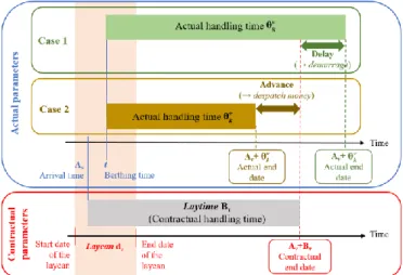
the cargo volume divided by the contractual rate of loading or unloading. If the charterer exceeds the laytime, a predetermined penalty called "demurrage" is incurred. This penalty equals the time exceeded multiplied by the demurrage rate. Otherwise, if the whole period of laytime is not needed, a refund called "despatch" may be payable by the shipowner to the charterer. This refund equals the time advanced multiplied by the despatch rate. Despatch is normally paid at 50% of the demurrage rate "Despatch half Demurrage", but this depends on the terms of the Charter Party. The vessel may thus be able to leave port early. These chartering terms are shown in Fig. 1.
Fig. 1. Comparison between the contractual and the actual parameters.
The Laycan Allocation Problem (LAP) refers to the problem of assigning berthing time windows to vessels within a medium-term planning (several weeks), by taking into
consideration commercial, logistical and production
constraints like sales forecasts, availability of cargo and production planning, due dates and quays availability, hence its interaction with the Berth Allocation Problem.
The Berth Allocation Problem (BAP) refers to the problem of assigning berthing positions and times to every vessel projected to be served within a short-term planning horizon (several days), such that a given objective function is optimized. The assignment must respect the constraints of the problem (vessels’ drafts and lengths, expected arrival times and projected handling times, etc.).
The integrated Laycan and Berth Allocation Problem (LBAP) considers the LAP and the BAP together. The combined problem aims to find an efficient schedule for berthing chartered vessels and new vessels to charter. It has to be noted that the freight transport is hardly predictable as many disturbances may occur (e.g., vessel delays, bad weather, etc.), thereby disabling the scheduled berth plan. Therefore, the LBAP should be solved on a rolling horizon. Indeed, each time a change occurs in the inputs of the problem (e.g., arrival and handling times of vessels, etc.), the model must be run again.
The paper is organized as follows. A literature review of the BAP and the LAP is presented in Section 2. The characteristics and the description of the mathematical model of the LBAP are presented in Section 3. An illustrative example and several numerical tests are provided in Section 4. Finally, in Section 5, we draw some conclusions and indicate future research.
II. LITERATURE REVIEW
The BAP has been widely studied by the scientific community. However, bulk terminals have received less attention than container terminals in the operational research literature. According to Bierwirth and Meisel [1], [2], the BAP models can be classified within four attributes: spatial, temporal, handling time and performance measure. We can add a fifth attribute that concerns the modeling of the BAP like the type of spatial and temporal constraints and the number and the type of variables used in the model (discrete, continuous, binary or a mix of these variables).
Most of authors solve the BAP using exact methods ranging from MILP formulations combined with standard solvers to highly sophisticated branching-based algorithms, heuristics like Genetic and Evolutionary Algorithms [3], and metaheuristics like Tabu Search [4] and Simulated Annealing [5].
Regarding the LAP, Lorenzoni et al. [6] proposed a tool based on a mathematical model of the LAP as a multi-mode resource-constrained scheduling problem. The tool determines laycans to vessels under the condition that once the vessels have arrived at the port, they have to be attended in first come first served order. They solved the problem using a heuristic procedure based on the Differential Evolution Algorithm. However, they only proposed a temporal allocation of port resources in general.
To the best of our knowledge, in the previous studies, the LAP and the BAP are solved separately. In this paper, we propose a mixed zero-one linear model for solving a new problem that combines the LAP and the BAP: the LBAP.
III. MATHEMATICAL MODEL FOR THE INTEGRATED LAYCAN
AND BERTH ALLOCATION PROBLEM
A. Characteristics of the Model 1) Spatial attribute
We consider a continuous berth layout (partitioned into a set of short length sections) with water depth restrictions (i.e.
all the sections of a quay can have the same water depth or the water depth increases seaward). We also take into consideration the technical constraints of vessels that prohibit their berthing at some quays or oblige them to berth at a specific quay.
2) Temporal attribute
We assume dynamic vessel arrivals with a maximum waiting time in harbor for each vessel (i.e. maximum berthing date of the vessel after its arrival to the port).
3) Handling time attribute
Handling times of vessels depend on their berthing positions. This variation can be due to the characteristics of the available equipment at the occupied sections (quay cranes, conveyors for bulk, internal transfer vehicles for containers, etc.). If a quay is divided into zones that have equipment with different productivities, we will consider that a vessel must berth at sections with equal productivities. In this case, the berth layout becomes almost hybrid in the sense that more than one vessel can berth at the same zone of the quay (without overlapping) but a vessel cannot berth at two different zones at the same time. This simplifying assumption can be subsequently withdrawn.
The laytime of a vessel is considered as its longest handling time in the port. The vessels which are already berthed in the port have fixed berthing times and positions and residual handling times.
4) Performance measure attribute
The objective is to achieve an optimal berth plan that reduces the late departures of chartered vessels by maximizing the difference between their despatch money and demurrage charges, while favoring their berthing as close as possible to the port yard. Furthermore, laycans are proposed for the new vessels to charter by making them leave the port as early as possible and berth as close as possible to the port yard without impacting the economic results of the chartered vessels.
B. Description of the Model 1) Input data
We consider a planning horizon divided into T periods (t =1,..., T) (e.g., days) and a port with Q quays (q =1,..., Q) partitioned into a set of short length sections (e.g., 10 m) in order to be in the continuous berth layout case. Each quay has a length of Sq sections (s =q 1,...,S );q by convention, the first section is the section that is closest to the port yard.
A vessel can berth at a section if the water depth is greater than its draft. We hence define H water depth and draft classes(h =1,..., H);by convention, the water depth of sections increases as h increases. The water depth of the section sq is
Jsq q .
Because the vessel handling times depend on the vessel berthing positions, we also define K productivity classes to
sections (k =1,..., K); by convention, the productivity of
sections increases as k increases. The productivity of the section sq is L .sq
We consider V1 berthed vessels (v =1,..., V ),1 V2 chartered vessels to berth (v =V1+1,..., V1+V )2 and V3 new
vessels to charter (vessels with unfixed laycans)
1 2
(v =V +V +1,..., V), where V=V1+V2+V .3 The berthing
of a vessel v at a quay q is subject to its technical constraints defined by the Boolean parameter Fqv (1 if vessel v can berth at quay q, 0 otherwise). Each vessel is characterized by an
estimated time of arrival Av (expressed as a number of
periods), a length λv (expressed as a number of sections) and
a draft Iv.
The handling time θv
k of a vessel v depends on the
productivity class Lsq
q
k = of the berthing position of its bow at
the section sq ( L θsq q v ). The 1
V berthed vessels have residual handling times, and fixed berthing times and positions. Each of the V2 chartered vessels has a laytime Bv =max (θ )k vk , a daily despatch rate α1v, a daily demurrage rate α2v, and a
maximum waiting time in harbor av provided that:
Av+av+Bv− 1 T. The role of this latter parameter is to reduce the solution space of berthing times in the planning horizon T. Therefore, the length of T does not influence the computation time of the model and its results.
Finally, the V3 vessels with unfixed laycans are handled as follows in the model: we assume that they have estimated times of arrival equal to availability dates of cargo to be exported. The number of days dv of the laycan of vessel v is included in its handling time. They also have fictitious daily despatch and demurrage rates equal to one and high maximum waiting times in harbor, so as not to affect the economic results of the V2 chartered vessels (despatch and demurrage).
2) Decision variables
Each vessel v arriving in the port can wait in the harbor before berthing at a time and a position. So we define the binary decision variable sq
vtq
x that equals one if the vessel v berths at the beginning of the period t and occupies the sections of the quay q from sq to s +q λv−1, where sq is the section occupied by its bow. The existence of the decision variable sq
vtq
x is subject to five conditions:
• The vessel v should berth after its estimated time of
arrival Av within the maximum waiting time in harbor,
denoted a :v Av t Av+av.
• The vessel v should be able to berth at the quay q:
Fv 1.
q =
• The length of the vessel v, denoted λv, should not exceed the limits of the quay q: s q Sq−λv+1. • The draft of the vessel v, denoted Iv, should not exceed
the water depth of the section of the berthing position
of its bow sq: I Jsq
v q . If this condition is verified for the first section sq, it will be implicitly verified for the other sections occupied by the vessel because the water depth of sections increases seaward.
• All sections occupied by the vessel v should have the same productivity class. Hence, the productivity classes of the two sections that have the berthing positions of the vessel’s bow and stern should be equal:
λ 1 Lsq Lsq v .
q q
+ − =
The logical condition of the existence of the decision variable sq
vtq
x is the following one:
λ 1 A A a F 1 S λ 1 I Jq Lq Lq v , v v q q v v s s s v v q q q q t s + − v + = − + = V
Conditioning the existence of the decision variable sq vtq
x to the respect of the five conditions described above improves significantly the computational performance of the model since it is no longer necessary to introduce them as constraints in the model.
To determine if a demurrage is incurred or a despatch money is to be collected, we need to know if a vessel is late or in advance, regarding its contractual departure time. Therefore, we introduce two variables: uv for the delay of a vessel v (i.e., end of handling time > end of laytime) and wv
for its advance (i.e., end of handling time < end of laytime).
3) Constraints
If a vessel v berths at the quay q, it can only have one berthing time t and one berthing position of its bow sq . Constraint (1) makes it possible that the problem might not necessarily lead to a solution where all vessels berth, as a strict equality enforces the berthing of all vessels.
λ 1 a F 1 S λ 1 I J L L 1, (1) q s s s v q q q v v v v q q q q v v q q q s vtq t A +t A q = s s − + = + − x v
VAs mentioned before, the V1 berthed vessels will have residual handling times and fixed berthing times
(
t =1)
andpositions with sq 1, 1.
vtq
x = V v
If a vessel v berths at the beginning of the period t, at the
quay q and its bow occupies the section sq that has a
productivity class Lsq
q
k = ( sq 1) vtq
x = , this vessel will occupy
the sections from sq =sq to sq = + −sq λv 1 during the periods from t =t to L θ sq 1 q v t = +t − .
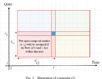
The constraint expressed in (2) and illustrated in Fig. 2, on the next page, is a spatiotemporal disjunctive constraint. It guarantees that a section cannot be occupied by more than one vessel at the same time by preventing overlap among the spatiotemporal rectangles representing vessels, which are located between sq = − +sq λv 1 and sq =sq on the spatial dimension, and between
L θ sq 1 q v t = −t + and t =t on the temporal dimension.
Fig. 2. Illustration of constraint (2).
To define the constraints of the variables uv and wv, we
use an intermediate variable, v, which gives the expected end
of handling time for a vessel v proposed by the model: λ 1 A A a F 1 S λ 1 I J L L ( θL 1) q s s s s v q q q v q v v v q qq q v v q q q q s v v t t q s s xvtq t =
+
= − + = + − + −The difference between the end of handling proposed by the model and the contracted handling deadline for vessel v can be written as −v (Av+Bv−1).The variables uv and wv should verify the constraints (3), (4) and (5) in order to determine the delay or the advance of each vessel.
(A B 1) 0 ( (A B 1)) 0 (A B 1) v v v v v v v v v v v v v v v u u w w u w − + − − − + − − = − + − (3) (4) (5) 4) Objective function
If −v (Av+Bv− 1) 0 , the vessel is overdue, the charterer will have to pay demurrage to the shipowner that is equal to α2vuv; otherwise, the vessel is in advance, the shipowner will have to pay despatch money to the charterer that is equal to α1vwv. Indeed, the charterer can benefit from a despatch money if the vessel berths as early as possible at sections with high productivity. In this case, the vessel’s handling time will be lower than its laytime.
The objective function expressed in (6) at the bottom of this page aims to maximize the difference between the despatch money and the demurrage of each chartered vessel, favors their berthing as close as possible to the port yard and
proposes laycans for new vessels to charter by making them leave the port as early as possible and berth as close as possible to the port yard without impacting the economic results of the chartered vessels.
The role of
2 3 1 2 (αv v αv v) v Max
w − u V V is to favordespatch money over demurrage charges for the V2 chartered
vessels and to make the V3 new vessels to charter leave the
port as early as possible. The role of Z in
(
)
λ 1
2 3 A A a F 1 S λ 1 I J L L Z 1/ q s s s v q q qv v v v q qq q v v q q q s vtq q v t t q s s Max
V V
+
= − + = + −x + sis to force berthing of all vessels (if possible), and the role of 1 /sq is to make vessels berth as close as possible to the port
yard in order to select one of the optimal economical solutions.
The laycan of the vessel v has a start date equal to its berthing time t proposed by the model and an end date equal to (t +dv−1) : laycan=
t t, +dv−1 .
The maximum waiting time in harbor av to negotiate with the shipowner should be greater than or equal to the waiting time in harbor proposed bythe model: av −t A .v Thereafter, we can assign daily
demurrage and despatch rates not equal to one to each new vessel to charter in order to see their impact on the economic criteria of the objective function. Therefore, it’s the decision-maker who will see how much he can accept the deterioration of the economic results.
IV. ILLUSTRATIVE EXAMPLE AND NUMERICAL TESTS
A. Illustrative Example
We consider a planning horizon divided into T=50 days
and a port of Q= quays. Each quay has a maximum length 3
1
(S =40, S2 =50 and S3=60 sections of 10 meters each).
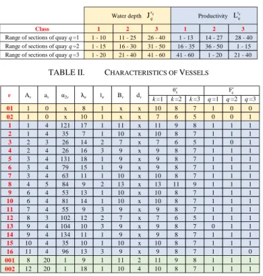
We define K=3 productivity classes to sections and H=3 draft and water depth classes to vessels and sections.
We consider V1=2 berthed vessels ( sq1,1 1, 1 1 v t q x= == = = and 21 1, 1, 3 1), q s v t q
x= == = = V2 =16 vessels to berth and V3 =2 vessels
with unfixed laycans. The daily despatch rates are half the
daily demurrage rates (α1v=α / 2)2v and the constant
Z = 10 000. The detailed characteristics of sections and
vessels are shown in Table I and Table II on the next page. In this example, the LBAP model uses 4 826 variables and 5 750 constraints. It’s computation time with Xpress in a PC of these characteristics (Intel® Xeon® CPU E3-1 240 v5 @ 3.50 GHz - 64 Go RAM) is 1 s. λ 1 λ 1 L S λ 1 I J L L A a F 1 λ 1 1 I J L L θ 1 A 1 2 S λ 1 I J L
1,
,
, s
α
α
(Z 1/ )
sq sq sq v q q q q v v q q q v v q v sq sq sq v v q q q v q v q q q sq v q q sq q q q v v q s s s t t t s vt q q v s s s t t t s v v v v s s vtq qx
t
q
Max
w
u
x
s
+ − + − = − + = = + = = − + = = − + − +
−
+
+
V
λ 1 2 3 A A a F 1 L s s v q q v v v v q q q v t t + q = = + −
V V
(2)
(6)
TABLE I. CHARACTERISTICS OF SECTIONS
1 2 3 1 2 3
1 - 10 11 - 25 26 - 40 1 - 13 14 - 27 28 - 40
1 - 15 16 - 30 31 - 50 16 - 35 36 - 50 1 - 15
1 - 20 21 - 40 41 - 60 41 - 60 1 - 20 21 - 40
Range of sections of quay q =3
Water depth Productivity
Class
Range of sections of quay q =1 Range of sections of quay q =2
Jsq
q L
q
s q
TABLE II. CHARACTERISTICS OF VESSELS
k =1 k =2 k =3 q =1 q =2 q =3 01 1 0 x 8 1 x x 10 8 7 1 0 0 02 1 0 x 10 1 x x 7 6 5 0 0 1 1 1 4 121 17 1 11 x 11 9 8 1 1 1 2 1 4 35 7 1 10 x 10 8 7 1 1 1 3 2 3 26 14 2 7 x 7 6 5 1 0 1 4 2 4 26 16 3 9 x 9 8 7 1 1 1 5 3 4 131 18 1 9 x 9 8 7 1 1 1 6 3 4 79 15 1 9 x 9 8 7 1 1 1 7 3 4 63 11 1 10 x 10 8 7 1 1 1 8 4 5 84 9 2 13 x 13 11 9 1 1 1 9 6 4 53 13 1 10 x 10 8 7 1 1 1 10 6 4 81 14 1 10 x 10 8 7 1 1 1 11 7 4 55 9 3 9 x 9 8 7 1 1 1 12 8 3 102 12 2 7 x 7 6 5 1 1 1 13 9 4 104 10 3 9 x 9 8 7 0 1 1 14 9 4 134 11 1 9 x 9 8 7 1 1 1 15 10 4 35 10 1 10 x 10 8 7 1 1 1 16 11 4 96 13 3 9 x 9 8 7 1 1 0 001 8 20 1 9 1 11 2 11 9 8 1 1 1 002 12 20 1 18 1 10 4 10 8 7 1 1 1 v Av av α2v λv Iv Bv dv θv k F v q
For the V2 chartered vessels, the sum of demurrage equals
442 against a sum of despatch equal to 843.5 and the sum of 1/sq is 5.4599. For the V3 vessels with unfixed laycans, the
sum of α1vwv−α2vuv is −2 and the sum of 1/sq is 0.09375.
Fig. 3 shows the disposition of the V1 berthed vessels, the
2
V chartered vessels, and the V3 vessels with unfixed
laycans, and the detailed results are shown in Table III.
TABLE III. RESULTS OF THE LBAP
v Av t Bv Av+Bv . q sq λv Demurrage vs Despatch Laycan 01 1 1 x 10 x 1 8 x x 3 2 2 7 6 1 14 14 13 x 7 3 3 10 7 3 28 11 94.5 x 12 8 8 7 6 1 14 12 51 x 15 10 11 10 10 -1 1 10 -35 x 16 11 11 9 7 2 28 13 96 x 2 1 1 10 8 2 36 7 35 x 5 3 3 9 9 0 16 18 0 x 6 3 3 9 7 2 1 15 79 x 10 6 10 10 7 -1 1 14 -81 x 13 9 9 9 8 1 36 10 52 x 002 12 12 10 10 0 16 18 x [12,15] 02 1 1 x 5 x 21 10 x x 1 1 1 11 9 2 1 17 121 x 4 2 2 9 9 0 41 16 0 x 8 4 4 13 9 4 32 9 168 x 9 6 10 10 8 -2 1 13 -106 x 11 7 11 9 9 -4 41 9 -220 x 14 9 9 9 7 2 21 11 134 x 001 8 13 11 8 -2 32 9 x [13,14] 1 2 3 - -θv k t θv k B. Numerical Tests
Most instances for the BAP published in the literature consider just one quay and do not have the same problem characteristics mentioned here. Frojan et al. [7], for instance, solved the BAP with multiple quays, but they considered fixed handling times for vessels and they did not consider water depth restrictions. Due to such differences, the comparison with the existing literature is difficult and can only be done for the simplified settings, which would lack relevance regarding this study. In order to evaluate the quality of the LBAP model, we have generated a set of instances with different sizes:
2 1 3
V = 20,30, 40,50 V = 2 V = 0, 2 (V3 = →0 BAP) and
Q= 1,3,5 .For all the instances, we consider a planning
horizon T=60 days and quays with different lengths
discretized in units of 10 meters.
The data relating to each vessel are drawn randomly from uniform distributions as follows: U
1,30
for arrival times,
7, 20
U for lengths, U
7,13
for laytimes, U
2, 4 forlaycan periods, U
1,3 for drafts and U
20,150
for dailydemurrage rates. The Boolean parameter Fv 0
q = for some
vessels. The maximum waiting time in harbor is determined
by applying this criterion: a 0.5 min θ ,v
v= k k rounded up to
the next integer (inspired by the criterion of the desired departure time sets by Bierwirth and Meisel [8]). TheV3 vessels with unfixed laycans have fictitious despatch and demurrage rates equal to one and high maximum waiting
times in harbor (av =20). The handling time of vessels
decreases by 20% from the productivity class k to k + , 1 rounded up to the next integer.
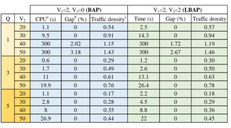
TABLE IV. RESULTS OF THE NUMERICAL TESTS
Q V2 CPUa (s) Gapb (%) Traffic densityc Time (s) Gap (%) Traffic density
20 1.1 0 0.54 2.5 0 0.57 30 9.5 0 0.91 14.3 0 0.94 40 300 2.02 1.15 300 1.72 1.19 50 300 3.18 1.43 300 2.67 1.46 20 0.6 0 0.29 1.2 0 0.30 30 1.7 0 0.49 2.6 0 0.50 40 11 0 0.61 13.1 0 0.63 50 19.9 0 0.76 26.4 0 0.78 20 1.1 0 0.17 2.2 0 0.18 30 2.8 0 0.28 4.5 0 0.29 40 8 0 0.35 8.8 0 0.36 50 26.9 0 0.44 22 0 0.45 V1=2, V3=2 (LBAP) 1 3 5 V1=2, V3=0 (BAP) a.
Computation time is limited to 300 s.
b.Gap=(ub lb− ) 100 / ub,
where ub is the value of the best upper bound obtained by considering all the decision variables as continuous, and lb is the value of the objective function corresponding to the best integer solution achieved within the time limit.
c.Traffic density =
(vλ B ) / (Tv k qS ).q This indicator measures the maximum spatiotemporal
occupations of vessels within the planning horizon and quay spaces (but does not include the arrival times of vessels which have a significant impact on the computation time). A traffic density higher than one means that the port cannot handle all vessels during the predefined planning horizon. V. CONCLUSION
In this paper, we propose a mixed zero-one linear model to solve a new problem called the integrated Laycan and Berth Allocation Problem. So, we combined the Laycan Allocation Problem and the Berth Allocation Problem which is one of the most important problems confronted at the quayside of ports. We apply the model in a port with multiple quays. Each quay has a continuous berth layout. We take into consideration quays’ water depths and vessels’ drafts and their technical constraints that prohibit the berthing of vessels in some quays or oblige them to berth at a specific quay. We also consider dynamic arrival times of vessels with a maximum waiting time in harbor for each vessel. Handling times of vessels depend on their berthing positions and the objective function aims to achieve an optimal berth plan that reduces the late departures of chartered vessels by maximizing the difference between their despatch money and demurrage charges, while favoring
their berthing as close as possible to the port yard, and to propose laycans for the new vessels to charter by making them leave the port as early as possible and berth as close as possible to the port yard without impacting the economic results of the chartered vessels.
The LBAP model uses one binary variable to determine the spatiotemporal allocations of vessels and two continuous variables that have integer values to determine if a demurrage is incurred or a despatch money is to be collected, and the spatiotemporal constraints are covered by a disjunctive constraint. The model is applied on a dataset where all the constraints are verified and its solving with Xpress is fast. This preliminary test enables us to validate the model. Other numerical experiences on instances with different sizes were done in order to evaluate the performance of the model and identify its limits.
It has to be noted that the optimal solutions proposed by the model may be unfeasible because of the unavailability of cargo to be exported in vessels (phosphate and its derivatives in the case of OCP Group): in practice, there is a strong interaction between vessels’ loading and production, unless an important decoupling of these problems is done by high stock levels, which is an expensive solution. So, as a perspective, we will develop a decision support system (DSS) to integrate the different port problems of allocation and scheduling, all in taking into account the constraints of the upstream supply chain. This DSS would follow an approach that combines optimization and simulation.
References
[1] C. Bierwirth and F. Meisel, “A survey of berth allocation and quay crane scheduling problems in container terminals,” European Journal of
Operational Research, vol. 202, no. 3, pp. 615–627, May 2010.
[2] C. Bierwirth and F. Meisel, “A follow-up survey of berth allocation and quay crane scheduling problems in container terminals,” European
Journal of Operational Research, vol. 244, no. 3, pp. 675–689, Aug.
2015.
[3] J. Karafa, M. M. Golias, S. Ivey, G. K. D. Saharidis, and N. Leonardos, “The berth allocation problem with stochastic vessel handling times,”
The International Journal of Advanced Manufacturing Technology, vol.
65, no. 1–4, pp. 473–484, Mar. 2013.
[4] G. Giallombardo, L. Moccia, M. Salani, and I. Vacca, “Modeling and solving the Tactical Berth Allocation Problem,” Transportation
Research Part B: Methodological, vol. 44, no. 2, pp. 232–245, Feb.
2010.
[5] S.-W. Lin and C.-J. Ting, “Solving the dynamic berth allocation problem by simulated annealing,” Engineering Optimization, vol. 46, no. 3, pp. 308–327, Mar. 2014.
[6] L. L. Lorenzoni, H. Ahonen, and A. G. de Alvarenga, “A multi-mode resource-constrained scheduling problem in the context of port operations,” Computers & Industrial Engineering, vol. 50, no. 1–2, pp. 55–65, May 2006.
[7] P. Frojan, J. F. Correcher, R. Alvarez-Valdes, G. Koulouris, and J. M. Tamarit, “The continuous Berth Allocation Problem in a container terminal with multiple quays,” Expert Systems with Applications, vol. 42, no. 21, pp. 7356–7366, Nov. 2015.
[8] F. Meisel and C. Bierwirth, “Heuristics for the integration of crane productivity in the berth allocation problem,” Transportation Research
Part E: Logistics and Transportation Review, vol. 45, no. 1, pp. 196–