A novel (3T-2R) parallel mechanism with large operational workspace and rotational capability

HAL Id: lirmm-01275355

https://hal-lirmm.ccsd.cnrs.fr/lirmm-01275355

Submitted on 1 Dec 2018

HAL is a multi-disciplinary open access

archive for the deposit and dissemination of

sci-entific research documents, whether they are

pub-lished or not. The documents may come from

teaching and research institutions in France or

abroad, or from public or private research centers.

L’archive ouverte pluridisciplinaire HAL, est

destinée au dépôt et à la diffusion de documents

scientifiques de niveau recherche, publiés ou non,

émanant des établissements d’enseignement et de

recherche français ou étrangers, des laboratoires

publics ou privés.

operational workspace and rotational capability

Samah Aref Shayya, Sébastien Krut, Olivier Company, Cédric Baradat,

François Pierrot

To cite this version:

Samah Aref Shayya, Sébastien Krut, Olivier Company, Cédric Baradat, François Pierrot. A novel

(3T-2R) parallel mechanism with large operational workspace and rotational capability. ICRA:

In-ternational Conference on Robotics and Automation, May 2014, Hong Kong, China. pp.5712-5719,

�10.1109/ICRA.2014.6907699�. �lirmm-01275355�



Abstract—The paper presents a novel 5 dofs (3T-2R) parallel mechanism. The mechanism is characterized by large singularity-free workspace and particularly large rotational capability which makes it suitable for 5 face-machining and similar applications. Having all its prismatic actuators along x direction, the x-motion is independent from other dofs-only limited by prismatic actuators’ strokes- constituting another major advantageous feature. Besides, an analytical direct geometric model can be easily established which is a rare feature in parallel robots. The paper introduces the novel mechanism with its inverse and direct geometric models as well as its kinematic models (forward and inverse Jacobians). Also, it discusses its singularity analysis and presents sample workspace plots evaluated based on isotropic performance regarding velocity and static force.

I. INTRODUCTION

To cope up with actual industrial needs, a research trend towards the synthesis of lower mobility parallel mechanisms has been noticed in the last decades. In fact, having a 5 dofs (3T-2R) mechanism is sufficient for the majority of industrial applications, such as machining, drilling, laser and water-jet cutting, etc. -even fewer number of dofs in others might be sufficient. These 5 dofs in general can be obtained either in one parallel architecture, via hybridization (parallel-series mechanisms), or through implementing right-hand left-hand paradigm.

Hybridization [1-2] is not a recommendable choice as it increases the moving mass (due to having additional actuators on the platform) and thus impacting dynamical performance as well as the global precision and stiffness of the robot.

On the other hand, right-hand left-hand paradigm might be more recommended and favored over hybridization, especially if 4 dofs are embedded in one parallel module (right-hand) and the remaining 1 dof is provided by separate left-hand mechanism: as for instance the suggested use of ARROW mechanism (3T-1R) studied in [3] with a turntable to provide the 2nd rotational dof. Other machines already

* This work has been supported partially by the French National Research Agency within the ARROW project (ANR 2011 BS3 006 01) and by Tecnalia France.

(a)-Tecnalia France – MIBI Building, 672 Rue du Mas de Verchant,

34000 Montpellier, France. E-mails: samah.shayya/cedric.baradat@tecnalia.com.

(b)-Montpellier Laboratory of Informatics, Robotics, and Microelectronics (LIRMM in French), a cross-faculty research entity of the Montpellier University of Sciences and Technologies (UM2) and the French National Center for Scientific Research (CNRS), 161 rue Ada,

34095 Montpellier, France. E-mails: shayya/krut/company/francois.pierrot@lirmm.fr.

exist such as the VERNE machine of [4] (parallel module (3T) + (2R) turntable (series)) and the SPKM 165 of [5] ((2T-1R) parallel module + (1T-1R) table (series)). But unfortunately these [4-5] have rather limited workspace. In addition, such mechanisms are usually less flexible and might introduce challenges regarding control and motion planning. This is not to mention calibration related issues. Thus, in some applications the best solution would be to have 5 dofs (3T-2R) parallel mechanism as one structure.

In literature, there are numerous synthesis and studies on 5 dofs (3T-2R) robots such as in [6-10] and many others... However, most of these available mechanisms are either characterized by limited workspace especially regarding tilting capacity, presence of singularities, and/or complexity of design especially from manufacturability point of view. For example, although the regularity of the mechanisms in [6] is interesting simplifying their analyses, it unfortunately leads to reduced stiffness and precision as not all the kinematic chains cooperate in counteracting the load, and the precision along each axis is rather controlled by individual kinematic chain and individual actuator’s resolution. Besides, having prismatic joints along different directions reduces workspace and makes them less practical from industrial point of view. The mechanism in [8] provides 5 dofs (3T-2R) using redundant parallel module formed by two folding five-bar linkages set on two rotatable links and connected to the platform via universal joints and a 7th actuator can be added in series to provide the 6th dof (3rd rotational dof) if needed. The direct geometrical model can be analytically derived which is interesting, but still the rotational capabilities and workspace are limited and dependent on position, not to mention that having the platform held by two universal joints is a drawback as the stiffness might be reduced. Regarding [9], the mechanism is undeniably interesting as it is characterized by large tilting capacity. This not to mention that having the actuators along one direction increases the workspace along this direction. Moreover, having an analytical forward geometric model is an additional bonus. But maybe the only drawback in this mechanism is the presence of cable-pulley or gear mechanism which can impact the robot’s performance regarding precision and stiffness.

This paper presents a novel 5 dofs (3T-2R) parallel mechanism in the attempt to resolve the major problematics emphasized in the above argument. The mechanism in its current version implements rack-pinion sub-mechanism (which might indicate similar problems to [9]) to facilitate the study only, but this in fact can be replaced by any rigid linear-to-rotational motion transformation mechanism having no singularity in the required rotational range. Also, compared to that suggested in [9], it has fewer actuators and

A Novel (3T-2R) Parallel Mechanism with Large Operational

Workspace and Rotational Capability*

hence lower costs (motors’ costs form a very large proportion of the overall robot’s cost). The mechanism is characterized by large workspace and tilting capacity, improved kinetostatic performance and relatively high expected dynamic capabilities. The paper introduces the mechanism in (II) with its geometric parameters. The inverse geometric model (IGM) and direct geometric model (DGM) are established in sections (III) and (IV) respectively; while in section (V) the kinematic models and singularities are discussed. Section (VI) then presents sample workspace plots evaluated using isotropic velocity and force based index (same as that used in [3]). The paper is concluded in section (VII) with conclusions and perspectives for future work.

II. THE NEW MECHANISM AND ITS GEOMETRIC ELEMENTS

The graph diagram of the mechanism with a simplified functional CAD are shown in Fig. 1 and Fig. 2, respectively. Fig. 3 shows the dimensions of the platform and the two moving frames. The functioning of the mechanism is straightforward. Chains (III) through (V) cooperate to position the segment B B_{4 5} which is always vertical thanks to the constraining parallelograms (II) and (III); these parallelograms do not allow any rotation about any axis perpendicular to the z-axis of the base frame. Then, chains (I) and (II) together control the two rotational dofs _z about the z-axis of the base frame and _y about the y-axis of the frame

 

M_f (tool frame). This is done thanks to the rack-pinion mechanism shown in Fig.2-3, which by fixing the distance between B₁B₂ with respect to parallelogram vertical axis



B B_{4 5}



and rotating it controls the 1st rotation (i.e. _z). As for _y it is controlled by moving the rack which turns the pinion an angle proportional to the relative displacement between



B B_{4 5}



and B₁. Thus, the TCP position and the tool orientation are controlled.

It is worth mentioning that we have used a rack-pinion here for simplicity of the analysis, but in general it can be replaced by any rigid linear-to-rotational motion transformation system having no singularities within the required range of rotation for _y which is between -45° and +45°; this allows avoiding precision and stiffness problems due to backlashes in rack pinion mechanism as previously highlighted. The mechanism tilting capacities are between -90° and +-90° regarding _z and between -45° and +45° regarding _y which are enough for 5-face machining applications...Moreover, the x-motion is independent of the other dofs and only restricted by available stroke for the linear actuators.

Regarding technical issues, it is worth mentioning that the limitation of commercial spherical joints can be overcome by replacing each with three concurrent perpendicular revolute joints.

Finally, we introduce the geometric parameters of the mechanisms as follows:

Figure 1. Simplified graph diagram of the 5 dofs (3T-2R) parallel mechanism. P,S,U: stand for prsimatic, spherical and universal joints respectively. Gray box signifies that the joint is actuated while underlining

means that the joint is equipped with a position sensor.

Figure 2. Simplified CAD for clarification purpose only. The base frame axes x,y, and z are shown on the drawing together with point notations.

 L_i (i1...5): length of i-th arm with L₁L₂, and 3 4 L L . 



 

T



T , 1...5 i  xi yi zi  qi yi zi i A : with 1 2 y1 y y L   , y₃ y₄ L_y2, y₅ , 0 z₁z₂ L_z1, 3 4 0 z z  , and z₅  L_z2. 





T = ( 1...5) i xbi ybi zbi i B : coordinates of B in the _i

base frame. Note that



m m m



T

N N N

x y z



m

N is the

coordinates of an arbitrary point N with respect to moving frame m with mM_i, M_f . Note that regarding the parallelogram arms, the points A and _i B are those along _i

the imaginary mid-axes.

 Note that point B is along the vertical line passing 5

through B₃B₄, and it is not coincident with them in practice (it is practically not feasible as it causes collisions), however for simplifying the modelling, we assume that

3 4 5

B B B and we compensate the real vertical offset

4 5

||BB ||_real in the z-ordinate of point A . This also means ₅

that the triple spherical joint shown in Fig. 2 (which is intended as simple clarifying CAD drawing) can also be replaced (practically) by double spherical joint or its equivalent (connecting the lower rods of parallelograms (III) and (IV) to platform) and a third spherical joint or universal joint for connecting chain (V) to the platform: so the technical difficulty of realization of a triple spherical joint can be overcome.







T

x y z



P : is the TCP position. The robot’s pose is





T

z y

x y z  



x with _z the rotation about the z-axis of the moving frame

 

M_i and _y is the rotation angle about the y-axis of the moving frame (M_f). Denote





T z y    θ .  Denote by





T 1 5 q q 

q  the actuated joints’

positions vector and by q



q₁  q₅



T the joints’ velocities vector.

 e , x e , and y e : are the unit vectors along x, y and z axes z

of the base frame, respectively.

 Denote by



 

 



T

cos _z sin _z 0 

h

e the unit vector

along x-axis of frame

 

M_i and by

 

 





T

sin _z cos _z 0  

f

e the unit vector along y-axis

of

 

M_i and

 

Mf .

 Denote v P , θ



 _z  , and _y



_x



_vT _θT



T_.

 Denote Ω_{ }e_z e_f_ and Ω₁



ez 0_{3 1}



, then



w Ω θ (angular velocity of the tool (blue color) expressed

in the base frame) and w₁Ω θ (angular velocity of 1₁ st part of platform (green color) and of the rack expressed in the base frame).

 R , and z R are the rotation matrices about z, and y axes y

respectively. We also define: R R R the rotation matrix  z y

of the tool frame

 

Mf with respect to the base frame.  Platform parameters ( a , b , c , r and _p t ) are shown on _p

Fig. 3.

III. THE INVERSE GEOMETRIC MODEL (IGM)

After having defined the mechanism’s geometric elements, it is time to establish the IGM.

The robot’s pose x is known, so we proceed by getting the points C and D (contact point between rack and

pinion) as follows:   Mf C P R C (1) and p r   z D C e (2) where _CMf_{, and} p

r are known (refer to Fig. 3). As we

have now C , it is easy to get points B₃,...,B₅ by:

3  4  5   3 , where 3  4  5

i i i i

M M M M

z

B B B C R B B B B (3)

It is important to recall here that point B is practically ₅

on the vertical line passing through B₃B₄ but not coincident with them (to avoid collisions in practical case) as shown clearly in Fig. 2-3, but for simplifying the modelling we considered them coincident by compensating the real vertical offset in the z-ordinate of point A (as we already ₅

explained in the previous section).

Now to get the point B₁B₂, we use the following relation:





1 2  rpy h crp z

B B D e e (4)

As we have obtained all the points B , we use the _i

following relation to get A : _i

2 2 , 1...5 i i Li  i A B (5) Relation (5) gives:





2 2 _{( )}2_{, 1...5} i i bi i bi i bi i q x x  L  y y  z z i (6) We choose the assembly mode to satisfy:

x , 1...5 i i bi

q x   i (7)

The solution is then:





2 2 2 ) ( , 1...5 i i bi i bi i bi i q x x  L  y y  z z i (8)

Hence, the IGM of the new mechanism has been established.

IV. THE DIRECT GEOMETRIC MODEL (DGM) The direct geometric model DGM is most often difficult to establish analytically for parallel robots. However, in our case it is quite simple. In fact, we have all the coordinates of points , 1...5A_i  i , so we get first the coordinates

3 4  5

B B B , then B₁B . Due to space limitation, we ₂

will describe it briefly. Consider the following system of equations: 3 3 4 4 2 2 3 2 2 3 4 5 2 2 4 5 5 5 , where L L L         _  A B B B A B A B B (9)

Solving the intersection of the three spheres described by (9) , we get in general two possible solutions, call them 1

3 s B and 2 3 s

B . Then, the z-ordinate of the point B₁B₂ is

known and it is given by (refer to Fig.3):





1 2 3

b b b

z z z  c b (10)

Hence, we have two possible z-ordinates 1 1 s b z and 2 1 s b z corresponding to 1 3 s B and 2 3 s

B respectively. We also have:

2 2 1 1 1 1 2 2 2 2 2 2, where L L    _    B B A B B A (11)

Again, substituting (10) in (11), we get in general two solutions corresponding to each value of z , we call them _b1

11 12 1 , 1 s s B B (corresponding to 1 1 s b z ) and 21 22 1 , 1 s s B B

(corresponding to z_bs₁2). Thus, we have in general a set of four solutions, denote it by   S S S S



₁, ₂, ₃, ₄



with

1 11 1 3 , 1 s s  S B B , 1 2 12 3 , 1 s s  S B B , 2 3 21 3 , 1 s s  S B B , and 2 4 22 3 , 1 s s 

S B B . Among them, a unique solution which satisfies the assembly mode (condition (7)) exists and as a result we have all the points B_i, 1...5 i . Consider then the vector η which is the projection of B B in the xy-_{3 1} plane, i.e.:





T



_T



3 1 3 1 0 x y      z z η B B B B e e (12)

Then, we have R knowing: z









2 , ; atan y x z        (13) We then get: 3 z 3 p z r e         i M C B R B C D C (14)

The matrix RR R is then computed where z y R is y

known after getting _y via the following relation:









T 1 p y p c r r   DB   ez eh (15)

The TCP position is given by:





T

x y z

   Mf

P C R C (16)

The pose is then given by x



x y z z y



Tand the DGM is therefore established.

V. THE JACOBIANS

In order to study singularities and evaluate the performance of the robot, we need to establish the Jacobian matrix J or the inverse Jacobian matrix J . Thus, we m

need to get the relation between q and





T

z y

x y z  



x      where  and _z  are the _y angular velocities about the two perpendicular directions e z

and e (note that in this case geometric inverse and f

forward Jacobians are essentially the same as their corresponding analytical notions; for discussion on this matter refer to [11]).

So, we proceed by differentiating (5) with respect to time to get: T T _{, 1...5} i i i i A  i i B  i A B v A B v (17) We have: , 1...5 i qi  i A x v  e (18)

It remains to get v in terms of x . For B_i i1, 2, we have:

   





 1 1 1 3 3 1 3 3 , 1, 2 : 3 3 identity matrix

... : pre-cross product matrix

i i i i i i                  _{ }       _{ }        B D v v w DB v w PD w DB v PD Ω θ DB Ω θ I PD Ω θ DB Ω I N N

x

  

_

(19) Regarding 4 5 3  B  B B v v v , we have for i3, 4,5:  





1 1 1 3 3 i i i i            _   _ B C v v w CB v w PC w CB I PC Ω CB Ω

x

(20)

Regrouping (17) in a matrix form and using (18) through (20), we get:



q x

J q J x  (21)

The matrix J is given by: q



T



 

1 5 T diag ,..., , dim 5 5, , 1...5 i i i i           q x x q J n e n e J n A B (22) As for J , it is as follows: x

 





 





 





 





 





 

T T 1 1 1 T 1 2 2 T 2 3 3 3 4 1 T T 1 T T 1 T T 5 4 4 5 5 1 dim 5 5   _{ }       _{ }                    _{ }       _{ }    _{ }     x x n n PD Ω DB Ω n n PD Ω DB Ω J n n PC Ω CB Ω n n PC Ω CB Ω n n PC Ω CB Ω J (23) When -1 q

J exists (det

 

J_q 0), the inverse Jacobian J _m (q J x m  ) is given by:

 

-1 _{, dim 5 5}    m q x m J J J J (24)

Similarly, when J exists, the forward Jacobian J -1x

(x J q  ) is given by:

 

-1 -1 _{, dim 5 5}

 m x q  

J J J J J (25)

So far, we have established the forward and inverse Jacobian matrices J and J , after establishing the m

matrices J and q J . In what follows, we discuss the series x

and parallel type singularities of the mechanism at hand.

A. Series Type Singularities

Series-type singularity occurs when J becomes rank _q deficient i.e. when det

 

Jq 0; in such a case the end-effector might be fixed (x 0 ), but the actuators are capable of infinitesimal motion (q 0 ). This means:

 





T det 0 1,..., 5 ; 0 o o o i i i        q x x J n e n e (26)

Relation (26) shows that series singularity occurs when there is a completely stretched arm (arm in the yz plane) which implies that singularity if exists (corresponding pose is accessible), it will be on the boundary of the geometrically accessible region and thus forms no problem.

B. Parallel Type Singularities

As for parallel-type singularities, these occur when the matrix J becomes rank deficient; in such a case the x

actuators can be fixed (q 0 ), but still the end-effector is capable of infinitesimal motion (x 0 ). We will do linear operations on J to facilitate the study. The first operation is x

a change of the TCP to be confounded with C (this does not change the rank since it is mathematically described as adding linear combinations of some columns to a certain column)(1), and thus we obtain the following matrix:

(1) _Adding



T   



T 1 5 T  z  z PC e PC e n  n (linear combinations of

first three columns) to 4th _{column of}

x J and adding













T T 1 5 T  f  f PC e PC e n  n to 5th _{column of} x J .  





 























T T 1 1 1 T T 1 T T 1 T T 1 T T 5 1 T T T 1 1 1 T T 1 2 2 2 3 3 3 4 4 4 5 5 2 2 2 3 4 4 5 T T T 3 T T T T 5 0 0 0 p y p p y p r r r r a a a    _{ }     _{ }            _     _                      _    f h f h f f f n n CD Ω DB Ω n n CD Ω DB Ω M n n CB Ω n n CB Ω n n CB Ω n n e n e n n e n e n n e n n e n n e (27)

Regarding the parameters a and r , refer to Fig. 3. To _p

simplify the rank study of M , we make another linear operation by adding



T ₅T



T

1

an ef  an ef to 4 th

column of M which gives us the simplified matrix:









T T T 1 1 1 T T T T 2 2 3 4 5 T 2 T 0 0 0 0 0 0 p y p p y p a r r a r r       _               f h f h n n e n e n n e n e N n n n (28)

Then, it is sufficient to study the rank of the following two sub-matrices of N :













T 1 3 4 5 T T 1 2 2 1 2 T T p y p p y p a r r a r r    _          _       f h f h N n n n n e n e N n e n e (29)

The matrix N (equivalently M and J ) is singular when x

any of the two matrices N or ₁ N is singular (rank ₂ deficient). The matrix N is of full rank as long as the three ₁

arms, namely (III), (IV) and (V), are not coplanar, which is guaranteed within the geometrically accessible space excluding its boundary. Actually, the matrix N ₁ (equivalently J ) may become rank deficient only in one _x case; this is when all the aforementioned arms are in one plane which cannot be -due to the assembly mode (condition (7))- except the yz-plane and hence parallel-type singularity confounded with serial-type singularity which cannot occur except at boundary of the geometrically accessible workspace-provided that the corresponding pose is geometrically accessible. Regarding the rank of N , ₂ computing and simplifying its determinant, we get:

 



 









 



1 2 1 2 2 1 2 1 2 det p y x y y x f_x h_y f_y h_x p y x y y x e e e e a r n n n n a r n n n n           N (30)

Note that vect_x and vect_y mean x and y ordinates of vector

vect respectively. We have ar_p_y  , 0



45 ; 45



y



      (i.e. a



rp



/ 4). Then, the only case where N (equivalently ₂ J ) is singular is when _x



n n1x 2yn n1y 2x



 , meaning that when the projections 0 of arms (I) and (II) in the xy plane are collinear which is not possible except when both arms are in the yz-plane and thus a parallel-type singularity coincident with a series-type singularity. Again, such a situation cannot occur except on the boundary of the geometrically accessible workspace-if the corresponding pose is geometrically accessible in the first place.

So, in brief, in this section we have proved that both types of singularities if to exist they are necessarily on the boundary of the geometrically accessible workspace-provided that the corresponding poses are geometrically reachable-and thus form no problem. Also, any parallel-type singularity if present, it exists confounded with a series-type singularity. As a result, we guarantee the absence of singularities of all types within the geometrically accessible workspace excluding its boundary.

VI. WORKSPACE ANALYSIS

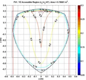
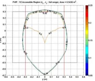
In this section, we present sample workspace analysis based on isotropic force-velocity performance index FVI

introduced in [3] that the reader may refer to. The index is defined as follows: min w, w wl wl v f FVI v f    _{ }   (31)

The terms v and _w f are the worst speed and the worst _w

force (2) respectively, whereas v and _wl f are the desired _wl

lower bounds for the worst speed and worst force respectively. Actually, v is nothing except the largest _w

isotropic speed (radius of the largest sphere included in the zonotope of the operational velocities), and f is similarly _w

the largest isotropic force (radius of largest sphere included in the operational force zonotope (refer to footnote (2))). In case of non-redundant robot, the pseudo-inverse is replaced by the usual matrix inverse. Actually, this index has been developed to overcome the loss of significance of singular values and based-upon indices (such as condition number, manipulability index, etc.) in case of redundant robots, but it is applicable to all types of robots and holds a concrete physical significance quantifying the maximal attainable

(2)

w

f is calculated considering minimum norm torque vector solution

of _ T

m

f J τ i.e. considering the joint torques vector τ satisfying

 

T T

null

  

 Jm  τ 0 and thus having:

T _ T  * m J f τ J f with  * m J J the

pseudo-inverse of J (case of redundancy) and f the operational force _m vector. Note to have physical significance and consistency of f , the _w matrix J must be homogeneous. _m

speed and maximal static force that can be supported by the end-effector regardless of direction. Furthermore, it serves as well as a singularity measure (closeness to singularity when

0

FVI )(3), although this latter significance is not our major concern or focus here as detailed analytical singularity analysis has been done in the previous section.

Since we have mixed dofs (translation and rotation), it is mandatory to homogenize J using a suitable technique m

before evaluating the index at each pose. Then, we consider the homogeneous inverse Jacobian matrix _ 1

mw m

J J W

and its pseudo-inverse J (in case of redundancy) or its w

inverse (i.e. the homogenized forward Jacobian

-1

 

w m

J W J W J ) as in our case here (non-redundancy).

Matrix W is the weighing or homogenization matrix and it is chosen here to be W diag 1,1,1, ,



a t_p



(the choice of the homogenization matrix is arbitrary with the condition that the weighing/homogenization matrix should assure that the initial (non-homogenized) and the corresponding homogenized matrices are of same rank where W is a square matrix: in our case we use the characteristic lengths technique). We then have:

1... 1.. m ax ax . m 1 min || || 1 min || || : number of actuators i i w w i m i m v q f m         _ _  _{ }         _{ }  _{ }   mwr wc j j  (32)

where jmwr_i and j are the i-th row vector and i-th wci

column vector of J_mw and J respectively. _w

In the figures that follow, we present the sample workspace plots and evaluation for the following geometric parameters (non-optimized parameters): L_i 1 , 1..5m  i ,

1 2 0.5 y y L L  m, L_z10.3m, L_z2 0.5m, a0.1m, 0.0875 b m, c0.125m, r_p 0.025m, t_p 0.075m, 0.0175 c m

t  , and t_l 0.2m. Note that t and _c t are the _l

minimum offsets from the sliders’ planes in case of zero rotation and full range of rotations, respectively.

Regarding the workspace plots, we have evaluated the yz-regions for zero orientation (_z _y  ) on one hand 0 and for full range rotations (i.e. _z     and



90 ; 90





45 ; 45



y

      ) on the other hand; this is since the inverse Jacobian is independent of x position. In case of full range orientation, we evaluated the index FVI for



90 , 60 , 45 , 30 , 0



z

        and _y 



45 , 30 , 0   being



frequently used orientations for the sake of reducing computation time, and the worst value of FVI (the lowest

(3) _{Note that when 0}

w

v  , it means approaching a series-type

singularity, while having f_w , it means approaching a parallel-type 0 singularity.

value) has been associated with the corresponding

 

y z , position. We have done the study on homogenized inverse Jacobian matrix J_mw (see Fig. 4-5) and a study considering only translational motion by considering the translational parts (4) of J and J , called m J and mp J respectively, p

which is the most interesting for us (regarding translational speed capability and pure static force capacity: see Fig. 6-7) as former study on J_mw can change with the chosen homogenization matrix W and its only importance is mainly as singularity performance measure (there is no real physical significance of studying the norm of 5 dimensional velocity vector composed by linear translation of a point and tangential velocity of another point with respect to the TCP; this is always the case when having mixed dofs irrespective of the index used). Note that considering translational performances only implies redundancy (3 dofs (3T) and 5 actuators, i.e. J and mp J are not square matrices). Note p

that the case of studying translational motion only implies that the angular velocity is controlled to be zero and there are no torques applied on the platform-i.e. we only have pure forces at the TCP). Also, it is worth mentioning that if singular values are significant regarding J_mw being a square matrix, singular values of J and _mp J are no more _p significant regarding output performance capabilities as explained in [12].

In all the plots, we have set v_wl  q_max and f_wl _max as to compare the isotropic velocity and force output performances of the mechanism relative to the maximal performances in velocity and force of the individual actuator (all actuators are considered identical). Note also that in the figures, the red solid lines show the collision limits with the sliders’ planes, while the dashed black box is the projection of the robot’s frame on the yz plane. The red lines are offset from vertical black dashed lines by t in case of zero _c

rotation and by t in case of full rotation. _l

Finally, to conclude up the section, it is clear that the mechanism has large singularity-free workspace considering zero rotation and full rotational capabilities. As a matter of fact, if we consider the ratio of the yz accessible region (with or without rotation) to the area of the black dashed box-representing the frame of the robot, this ratio is clearly high.

Besides, the kinetostatic performances are quite interesting (remember that these represent capabilities that can be achieved in all directions). It would even be more improved and its performance more enhanced after properly optimizing this mechanism which is not our concern here. Additionally, the workspace is convex; such convexity is important regarding trajectory planning where each two points can be joined by a straight line trajectory.

(4) _{In this case}

mw

J and J in relation (32) are respectively replaced by w

:, 1: 3



mp m

J J i.e. first three columns of J and m JpJ(1: 3,:) i.e.

first three rows of _ -1

m

J J (non-redundant robot) and  m

*

J J

(pseudo-inverse of J in case of redundancy). m

Figure 4. Geometrically accessible workspace for zero rotation: evaluated using index FVI(Jmw).

Figure 5. Geometrically accessible workspace with full rotational range: evaluated using FVI(Jmw).

Figure 6. Geometrically accessible workspace for zero rotation: evaluated using index FVIP (the P indicates study of positional parts of

Figure 7. Geometrically accessible workspace with full rotational range: evaluated using index FVIP (the P indicates study of positional parts of

inverse Jacobian Jm and forward Jacobian J matrices).

VII. CONCLUSION AND PERSPECTIVES

In this paper, we have introduced a novel 5 dofs (3T-2R) parallel mechanism that has the following characteristics:  The functioning of the mechanism is simple.

 It admits an analytical direct geometric model DGM that is a rare feature to find regarding parallel manipulators and can be very helpful regarding control issues.

 It has independent motion along x-direction only restricted by available stroke for prismatic joints.

 Parallel type singularities if to exist, they are coincident with series-type singularities and cannot occur except at the geometrically accessible workspace boundary (provided that corresponding poses are geometrically achievable). Thus, in any case they do not form any problem.

 It has large singularity-free cross-sectional workspace with or without rotation. Also, its isotropic kinetostatic performance is quite interesting and it is expected to be improved even more after optimization. This has been clarified by the preliminary analysis of workspace for non-optimized set of geometric parameters.

 High stiffness having all the limbs sharing in the load support along all directions.

 Having spherical joints at the arms’ extremities puts these arms under tension/compression forces which improves accuracy due to reduced deformation in the arms.

It is important to mention that this mechanism is a starting point, as other versions based on this one and with better performance are being thought of and may be the subject for future publications. We also emphasize that in this mechanism, the use of rack-pinion is meant to simplify the modelling and the preliminary presentation of the mechanism, but in the realistic case it would be replaced by

more rigid linear-to-rotational motion transformation mechanism.

REFERENCES

[1] Siciliano B., “The Tricept Robot: Inverse kinematics, manipulability analysis and closed-loop direct kinematics algorithm”, Robotica, pp. 437-445, 1999.

[2] Liu H., Huang T., Mei J.., Zhao X.., Chetwynd D. G., Li M., and Hu S. J. “Kinematic Design of a 5-DOF Hybrid Robot with Large Workspace/Limb–Stroke Ratio”, ASME Journal of Mechanical Design, 129 (5), pp. 530–538.

[3] Shayya S., Krut S., Company O., Baradat C., and Pierrot F., “A Novel (3T-1R) Redundant Parallel Mechanism with Large Operational Workspace and Rotational Capability”, in Proc. of IEEE/RSJ International Conference on Intelligent Robots and Systems, IROS 2013, pp. 436-443, Tokyo, Japan, November 3-8, 2013.

[4] Kanaan D., Wenger P. and Chablat D., “Kinematic Analysis of a Serial – Parallel Machine Tool: the VERNE machine”, Mechanism and Machine Theory, Vol. 44(2), pp. 487-498, February 2009. [5] Xie F-G., Liu X-J, Zhang H. and Wang J-S. , “Design and

experimental study of the SPKM165, a five-axis serial-parallel kinematic milling machine”, Science China Technological Sciences, May 2011, Volume 54, Issue 5, pp. 1193-1205.

[6] Gogu G., “Structural synthesis of maximally regular T3R2-type parallel robots via theory of linear transformations and evolutionary morphology”, Robotica (2009) volume 27, pp. 79–101.

[7] Motevalli B., Zohoor H., and Sohrabpour S., “Structural synthesis of 5 DoFs 3T2R parallel manipulators with prismatic actuators on the base”, Robotics and Autonomous Systems 58 (2010) 307–321. [8] Salcudean Septimiu E, Stocco Leo J, “Hybrid serial/parallel

manipulator”, U.S. patent: US6047610 A, April 11, 2000.

[9] Krut S., Company O., Rangsri S., and PIERROT F. “Eureka: A New 5-Degree-of-Freedom Redundant Parallel Mechanism with High Tilting Capabilities”, Proceedings of the 2003 IEEE/RSJ Intl. Conference on Intelligent Robots and Systems, Las Vegas, Nevada · October 2003.

[10] Bruzzone L., Molfino R., and Zoppi M., “Kinematic modelling and simulation of a novel interconnected-chains PKM”, in Int. Conf. Modelling, Identification and Control, MIC2004, Grindelwald, 23-25 February 2004.

[11] Siciliano B., Sciavicco L., Villani L., Oriolo G., “Robotics:

modelling, planning and control”, pp. 105-160, Springer, c2009. [12] Krut S., “Contribution à l’étude des robots parallèles légers, 3T-1R et

3T-2R, à forts débattements angulaires », Ph.D Thesis, Université Montpellier 2, Novembre 3, 2003.